Asymptotic normality of the mixture density estimator in a disaggregation scheme

Abstract

The paper concerns the asymptotic distribution of the mixture density estimator, proposed by Leipus et al., (2006), in the aggregation/disaggregation problem of random parameter AR(1) process. We prove that, under mild conditions on the (semiparametric) form of the mixture density, the estimator is asymptotically normal. The proof is based on the limit theory for the quadratic form in linear random variables developed by Bhansali et al., (2007). The moving average representation of the aggregated process is investigated. A small simulation study illustrates the result.

Keywords: random coefficient AR(1), long memory, aggregation, disaggregation, mixture density.

1 Introduction

Aggregated time series data appears in different fields of studies including applied problems in hydrology, sociology, statistics, economics. Considering aggregation as a time series object, a number of important questions arise. These comprise the properties of macro level data obtained by small and large-scale aggregation in time, space or both, assumptions of when and how the inverse (disaggregation) problem can be solved, finally, how to apply theoretical results in practice.

Aggregated time series, in fact, can be viewed as a transformation of the underlying time series by some (either linear or non-linear) specific function defined at (in)finite set of individual processes. In this paper we consider a linear aggregation scheme, which is natural in applications. In practice it is found convenient to approximate individual data by simple time series models, such as AR($1$), GARCH($1,1$) for instance (see Lewbel, (1994), Chong, (2006), Zaffaroni (2004, 2006)), whereas more complex individual data models do not provide an advantage in accuracy and efficiency of estimates, and usually are very difficult to study from the theoretical point of view.

Aggregation by appropriately averaging the micro level time series models can give intriguing results. It was shown in Granger (1980) that the large-scale aggregation of infinitely many short memory AR(1) models with random coefficients can lead to a long memory fractionally integrated process. It means that the properties of an aggregate time series may in general differ from those of individual data.

It is clear however that the weakest point of the aggregation is a considerable loss of information about individual characteristics of the underlying data. Roughly speaking, an aggregated time series can not be as informative about the attributes of individual data as the micro level processes are. On the other hand, using some special aggregation schemes, which involve, for instance, independent identically distributed “elementary” processes with known structure (such as AR($1$)), enables to solve an inverse problem: to recover the properties of individual series with the aggregated data at hand. This problem is called a disaggregation problem.

Different aspects of this problem were investigated in Dacunha-Castelle, Oppenheim (2001), Leipus et al., (2006), Celov et al., (2007). The last two papers deal with the asymptotic statistical theory in the disaggregation problem: they present the construction of the mixture density estimate of the individual AR(1) models, the consistency of an estimate, and some theoretical tools needed here. Resuming the previous research, the major objective of the present paper is to obtain the asymptotic normality property of the mixture density estimate, that enlarges the range of applications, solving the accuracy of simulation studies, statistical inference, forecasting and other problems.

Section 2 describes the disaggregation scheme, including the construction of mixture density estimate proposed by Leipus et al., (2006), and formulates the main result of the paper. Important issues about the moving average representation of the aggregated process are discussed in Section 3. The proof of the main theorem and auxiliary results are given respectively in Section 4 and Section 7. Some simulation results are presented in Section 5.

2 Preliminaries and the main result

Consider a sequence of independent processes $Y^{(j)}=\{Y^{(j)}_{t},t\in\bf Z\}$, $j\geq 1$ defined by the random coefficient AR(1) dynamics

$$Y_{t}^{(j)}=a^{(j)}Y^{(j)}_{t-1}+\varepsilon^{(j)}_{t},$$ (2.1)

where $\varepsilon^{(j)}_{t},\ t\in{\bf Z}$, $j=1,2,\dots$ are independent identically distributed (i.i.d.) random variables with $\mathrm{E}\varepsilon^{(j)}_{t}=0$ and $0<\sigma_{\varepsilon}^{2}=\mathrm{E}(\varepsilon^{(j)}_{t})^{2}<\infty$; $a,\,a^{(j)},\ j=1,2,\dots$ are i.i.d. random variables with $|a|\leq 1$ and satisfying

$$\mathrm{E}\Big{[}\frac{1}{1-a^{2}}\Big{]}<\infty.$$ (2.2)

It is assumed that the sequences $\{\varepsilon^{(j)}_{t},t\in{\bf Z}\}$, $j=1,2,\dots$ and $\{a,a^{(j)},j=1,2,\dots\}$ are independent.

Under these conditions, (2.1) admits a stationary solution $Y^{(j)}$ and, according to Oppenheim and Viano, (2004), the finite dimensional distributions of the process

$$X^{(N)}_{t}=\frac{1}{\sqrt{N}}\;\sum_{j=1}^{N}Y_{t}^{(j)},\ \ t\in{\bf Z},$$

weakly converge as $N\to\infty$ to those of a zero mean stationary Gaussian process $X=\{X_{t},t\in{\bf Z}\}$, called the aggregated process. Suppose that random coefficient $a$ admits a density $\varphi(x)$, absolutely continuous with respect to the Lebesgue measure, which by (2.2) satisfies

$$\int_{-1}^{1}\frac{\varphi(x)}{1-x^{2}}\ \mathrm{d}x<\infty.$$ (2.3)

Any density function satisfying (2.3) will be called a mixture density.

Note that the covariance function and the spectral density of aggregated process $X$ coincides with those of $Y^{(j)}$ and are given, respectively, by

$$\sigma(h):={\rm Cov}(X_{h},X_{0})=\sigma^{2}_{\varepsilon}\int_{-1}^{1}\frac{x^{|h|}}{1-x^{2}}\ \varphi(x)\mathrm{d}x$$ (2.4)

and

$$f(\lambda)=\frac{\sigma^{2}_{\varepsilon}}{2\pi}\int_{-1}^{1}\frac{\varphi(x)}{|1-x\mathrm{e}^{\mathrm{i}\lambda}|^{2}}\ \mathrm{d}x.$$ (2.5)

The disaggregation problem deals with finding the individual processes (if they exist) of form (2.1), which produce the aggregated process $X$ with given spectral density $f(\lambda)$ (or covariance $\sigma(h)$). This is equivalent to finding $\varphi(x)$ such that (2.5) (or (2.4)) and (2.3) hold. In this case, we say that the mixture density $\varphi(x)$ is associated with the spectral density $f(\lambda)$.

In order to estimate the mixture density $\varphi(x)$ using aggregated observations $X_{1},\dots,X_{n}$, Leipus et al., (2006) proposed the estimate based on a decomposition of function $\zeta(x)=\varphi(x)(1-x^{2})^{-\alpha}$ in the orthonormal $L^{2}(w^{(\alpha)})$–basis of Gegenbauer polynomials $\{G_{k}^{(\alpha)}(x),k=0,1,\dots\}$, where $w^{(\alpha)}(x)=(1-x^{2})^{\alpha}$, $\alpha>-1$. This decomposition is valid (i.e. $\zeta$ belongs to $L^{2}(w^{(\alpha)})$) if

$$\int_{-1}^{1}\frac{\varphi^{2}(x)}{(1-x^{2})^{\alpha}}\;\mathrm{d}x<\infty,\ \ \alpha>-1.$$ (2.6)

Let $G_{n}^{(\alpha)}(x)=\sum_{j=0}^{k}g^{(\alpha)}_{n,j}x^{j}$. The resulting estimate has the form

$$\hat{\varphi}_{n}(x)=\hat{\sigma}^{-2}_{n,\varepsilon}(1-x^{2})^{\alpha}\sum_{k=0}^{K_{n}}\hat{\zeta}_{n,k}G_{k}^{(\alpha)}(x),$$ (2.7)

where the $\hat{\zeta}_{n,k}$ are estimates of the coefficients $\zeta_{k}$ in the $\alpha$-Gegenbauer expansion of the function $\zeta(x)=\sum_{k=0}^{\infty}\zeta_{k}G_{k}^{(\alpha)}(x)$ and are given by

$$\hat{\zeta}_{n,k}=\sum_{j=0}^{k}g_{k,j}^{(\alpha)}(\hat{\sigma}_{n}(j)-\hat{\sigma}_{n}(j+2)),$$ (2.8)

$\hat{\sigma}^{2}_{n,\varepsilon}=\hat{\sigma}_{n}(0)-\hat{\sigma}_{n}(2)$ is the consistent estimator of variance $\sigma^{2}_{\varepsilon}$ and $\hat{\sigma}_{n}(j)=n^{-1}\sum_{i=1}^{n-j}X_{i}X_{i+j}$ is the sample covariance of the aggregated process. Truncation level $K_{n}$ satisfies

$$K_{n}=[\gamma\log n],\qquad 0<\gamma<(2\log(1+\sqrt{2}))^{-1}.$$ (2.9)

Leipus et al., (2006) assumed the following semiparametric form of the mixture density:

$$\varphi(x)=(1-x)^{1-2d_{1}}(1+x)^{1-2d_{2}}\psi(x),\ \ 0<d_{1},d_{2}<1/2,$$ (2.10)

where $\psi(x)$ is continuous on $[-1,1]$ and does not vanish at $\pm 1$. Then, under conditions above and corresponding relations between $\alpha$ and $d_{1},d_{2}$, they showed the consistency of the estimator $\hat{\varphi}_{n}(x)$ assuming that the variance of the noise, $\sigma^{2}_{\varepsilon}$, is known and equals 1. In more realistic situation of unknown $\sigma^{2}_{\varepsilon}$, it must be consistently estimated. In order to understand intuitively the construction of estimator $\hat{\sigma}^{2}_{n,\varepsilon}$, it suffices to note that, by (2.4), $\sigma^{2}_{\varepsilon}=\sigma(0)-\sigma(2)$. Also note that the estimator $\hat{\varphi}_{n}(x)$ in (2.7) possesses property $\int_{-1}^{1}\hat{\varphi}_{n}(x)\mathrm{d}x=1$, which can be easily verified noting that $\int_{-1}^{1}(1-x^{2})^{\alpha}G_{k}^{(\alpha)}(x)\;\mathrm{d}x=(g^{(\alpha)}_{0,0})^{-1}$ if $k=0$, and $=0$ otherwise, implying

$$\int_{-1}^{1}(1-x^{2})^{\alpha}\sum_{k=0}^{K_{n}}\hat{\zeta}_{n,k}G_{k}^{(\alpha)}(x){\rm d}x=\hat{\zeta}_{n,0}/g^{(\alpha)}_{0,0}=\hat{\sigma}_{n}(0)-\hat{\sigma}_{n}(2)$$

by (2.8).

In this paper, we further study the properties of the proposed mixture density estimator. In order to formulate the theorem about the asymptotic normality of estimator $\hat{\varphi}_{n}(x)$, we will assume that aggregated process $X_{t}$, $t\in{\bf Z}$ admits the following linear representation.

Assumption A  Assume that $X_{t}$, $t\in{\bf Z}$ is a linear sequence

$$X_{t}=\sum_{j=0}^{\infty}\psi_{j}Z_{t-j},$$ (2.11)

where the $Z_{t}$ are i.i.d. random variables with zero mean, finite fourth moment and the coefficients $\psi_{j}$ satisfy

$$\psi_{j}\sim cj^{d-1},\ \ |\psi_{j}-\psi_{j+1}|=O(j^{d-2}),\ 0<d<1/2$$ (2.12)

with some constant $c\neq 0$.

We also introduce the following condition on the mixture density $\varphi(x)$.

Assumption B  Assume that mixture density $\varphi$ has a form

$$\varphi(x)=(1-x)^{1-2d}\psi(x),\ \ 0<d<1/2,$$ (2.13)

where $\psi(x)$ is a nonnegative function with ${\rm supp}(\psi)\subset[-1,1]$, continuous at $x=1$, $\psi(1)\neq 0$.

Note that, omitting in (2.10) the factor responsible for the seasonal part, we thus obtain the corresponding ’long memory’ spectral density with singularity at zero (but not necessary at $\pm\pi$) and the corresponding behavior of the coefficients $\psi_{j}$ in linear representation (3.2).

Theorem 2.1

Let $X_{t},t\in{\bf Z}$ be the aggregated process satisfying Assumption A and corresponding to the mixture density given by Assumption B. Assume that (2.6) holds, and $d$ and $\alpha$ satisfy the following condition

$$-1/2<\alpha<\frac{5}{2}-4d.$$ (2.14)

Let $K_{n}$ be given in (2.9) with $\gamma$ satisfying

$$0<\gamma<(2\log(1+\sqrt{2}))^{-1}\Big{(}1-\max\Big{\{}\alpha+4d-\frac{3}{2},0\Big{\}}\Big{)}.$$ (2.15)

Then for every fixed $x\in(-1,1)$, such that $\varphi(x)\neq 0$, it holds

$$\frac{\hat{\varphi}_{n}(x)-\mathrm{E}\hat{\varphi}_{n}(x)}{\sqrt{{\rm Var}(\hat{\varphi}_{n}(x))}}\stackrel{{\scriptstyle\mbox{$\scriptstyle d$}}}{{\longrightarrow}}{\rm N}(0,1).$$ (2.16)

Proof of the theorem is given in Section 4.

Remark 2.1

Suppose that $\varphi(x)$ satisfies Assumption B. Then assumption (2.6) is equivalent to $\int_{-1}^{1}\psi^{2}(x)(1+x)^{-\alpha}\mathrm{d}x<\infty$ and $\alpha<3-4d$. The last inequality is implied by (2.14).

Example 2.1

Assume two mixture densities

$$\varphi(x;d)=C_{1}(d)x^{d-1}(1-x)^{1-2d}(1+x){\bf 1}_{(0,1]}(x),\ 0<d<1/2,$$ (2.17)

where $C_{1}(d)=\frac{\Gamma(3-d)}{2\Gamma(d)\Gamma(2-2d)}$, and

$$\varphi_{g}(x;\kappa)=C_{2}(\kappa)|x|^{\kappa}{\bf 1}_{[-a_{*},0]}(x),\ \ \kappa>0,$$ (2.18)

where $0<a_{*}<1$, $C_{2}(\kappa)=(\kappa+1)(a_{*})^{-\kappa-1}$.

According to Dacunha-Castelle and Oppenheim (2001), the spectral density corresponding to $\varphi(x;d)$ is FARIMA(0,$d$,0) spectral density

$$f(\lambda;d)=\frac{1}{2\pi}\ \Big{(}2\sin\frac{|\lambda|}{2}\Big{)}^{-2d}.$$ (2.19)

Also, since the support of $\varphi_{g}$ lies inside $(-1,1)$, the spectral density $g(\lambda;\kappa)$ corresponding to $\varphi_{g}(x;\kappa)$ is analytic function (see Proposition 3.3 in Celov et al., (2007)).

Consider the spectral density given by

$$f(\lambda)=f(\lambda;d)g(\lambda;\kappa),\ \ \lambda\in[-\pi,\pi].$$ (2.20)

It can be shown that the mixture density $\varphi(x)$ associated with $f(\lambda)$ (2.20) is supported on $[-a_{*},1]$, satisfies Assumption B with $\psi(x)$ which is continuous function on $[-a_{*},1]$ and at the neighborhood of zero satisfies $\psi(x)=O(|x|^{d})$. This implies the validity of condition (2.6) needed to obtain the corresponding $\alpha$-Gegenbauer expansion. For the proof of this example and precise asymptotics of $\psi(x)$ at zero see Appendix A.

Finally, the aggregated process $X$, obtained using such mixture density $\varphi(x)$, satisfies Assumption A by Proposition 3.2, which shows that assumptions A and B are satisfied under general ’aggregated’ spectral density $f(\lambda)=f(\lambda;d)g(\lambda)$, where $g(\lambda)$ is analytic function on $[-\pi,\pi]$ and the associated mixture density is supported on $[-a_{*},0]$ with some $0<a_{*}<1$.

Remark 2.2

Note that the ’FARIMA mixture density’ (2.17), due to factor $x^{d-1}$, does not satisfy (2.6) and a ”compensating” density such as $\varphi_{g}(x;\kappa)$ in (2.18) is needed in order to obtain the needed integrability in the neighborhood of zero. Obviously, for the same aim, other mixture densities instead of $\varphi_{g}(x;\kappa)$ (2.18) can be employed.

3 Moving average representation of the aggregated process

In order to obtain the asymptotic normality result in Theorem 2.1, an important assumption is that the aggregated process admits a linear representation with coefficients decaying at an appropriate rate (see Bhansali et al., (2007)). The related issues about the moving average representation of the aggregated process are discussed in this section.

From the aggregating scheme follows that any aggregated process admits an absolutely continuous spectral measure. If, in addition, its spectral density, say, $f(\lambda)$ satisfies

$$\int_{-\pi}^{\pi}\log f(\lambda)\mathrm{d}\lambda>-\infty,$$ (3.1)

then the function

$$h(z)=\exp\Big{\{}\frac{1}{4\pi}\int_{-\pi}^{\pi}\frac{\mathrm{e}^{\mathrm{i}\lambda}+z}{\mathrm{e}^{\mathrm{i}\lambda}-z}\;\log f(\lambda)\mathrm{d}\lambda\Big{\}},\ \ |z|<1,$$

is an outer function from the Hardy space $H^{2}$, does not vanish for $|z|<1$ and $f(\lambda)=|h(\mathrm{e}^{\mathrm{i}\lambda})|^{2}$. Then, by the Wold decomposition theorem, corresponding process $X_{t}$ is purely nondeterministic and has the MA($\infty$) representation (see Anderson (1971, Ch. 7.6.3))

$$X_{t}=\sum_{j=0}^{\infty}\psi_{j}Z_{t-j},$$ (3.2)

where the coefficients $\psi_{j}$ are defined from the expansion of normalized outer function $h(z)/h(0)$, $\sum_{j=0}^{\infty}\psi_{j}^{2}<\infty$, $\psi_{0}=1$, and $Z_{t}=X_{t}-\widehat{X}_{t}$, $t=0,1,\dots$ ($\widehat{X}_{t}$ is the optimal linear predictor of $X_{t}$) is the innovation process, which is zero mean, uncorrelated, with variance

$$\sigma^{2}=2\pi\exp\Big{\{}\frac{1}{2\pi}\int_{-\pi}^{\pi}\log f(\lambda)\mathrm{d}\lambda\Big{\}}.$$ (3.3)

By construction, the aggregated process is Gaussian, implying that the innovations $Z_{t}$ are i.i.d. N$(0,\sigma^{2})$ random variables.

Next we focus on the class of semiparametric mixture densities satisfying Assumption B. As it was mentioned earlier, this form is natural, in particular it covers the mixture densities $\varphi_{1}(x;d)$ and $\varphi(x)$ in Example 2.1.

Proposition 3.1

Let the mixture density $\varphi(x)$ satisfies Assumption B. Assume that either

(i) ${\rm supp}(\psi)=[-1,1]$ and $\tilde{\psi}(x)\equiv\psi(x)(1+x)^{2\tilde{d}-1}$ is continuous at $-1$ and $\tilde{\psi}(-1)\neq 0$ with some $0<\tilde{d}<1/2$,

or

(ii) ${\rm supp}(\psi)\subset[-a_{*},1]$ with some $0<a_{*}<1$.

Then the aggregated process admits a moving average representation (3.2), where the $Z_{t}$ are Gaussian i.i.d. random variables with zero mean and variance (3.3).

Proof. ($i$) We have to verify that (3.1) holds. Rewrite $\varphi(x)$ in the form

$$\varphi(x)=(1-x)^{1-2d}(1+x)^{1-2\tilde{d}}\tilde{\psi}(x).$$

Proposition 4.1 in Celov et al., (2007) implies

$$f(\lambda)\sim C_{1}|\lambda|^{-2d},\quad|\lambda|\to 0,$$

with $C_{1}>0$. Hence $\log f(\lambda)\sim\log C_{1}-C_{2}\log|1-\mathrm{e}^{\mathrm{i}\lambda}|$, $|\lambda|\to 0$, where $C_{2}>0$. For any $\epsilon>0$ choose $0<\lambda_{0}\leq\pi/3$, such that

$$-\frac{\log f(\lambda)-\log C_{1}}{C_{2}\log|1-\mathrm{e}^{\mathrm{i}\lambda}|}-1\geq-\epsilon,\ \ 0<\lambda\leq\lambda_{0}.$$

Since $-\log|1-\mathrm{e}^{\mathrm{i}\lambda}|\geq 0$ for $0\leq\lambda\leq\pi/3$, we obtain

$$\int_{0}^{\lambda_{0}}\log f(\lambda)\mathrm{d}\lambda\geq\lambda_{0}\log C_{1}-C_{2}(1-\epsilon)\int_{0}^{\lambda_{0}}\log|1-\mathrm{e}^{\mathrm{i}\lambda}|\mathrm{d}\lambda>-\infty$$ (3.4)

using the well known fact that $\int_{0}^{\pi}\log|1-\mathrm{e}^{\mathrm{i}\lambda}|\mathrm{d}\lambda=0$. Similarly,

$$\int_{\pi-\lambda_{0}}^{\pi}\log f(\lambda)\mathrm{d}\lambda>-\infty.$$ (3.5)

When $\lambda\in[\lambda_{0},\pi-\lambda_{0}]$, there exist $0<L_{1}<L_{2}<\infty$ such that

$$L_{1}\leq\frac{1}{2\pi|1-x\mathrm{e}^{\mathrm{i}\lambda}|^{2}}\leq L_{2}$$

uniformly in $x\in(-1,1)$. Thus, by (2.5), $L_{1}\leq f(\lambda)\leq L_{2}$ for any $\lambda\in[\lambda_{0},\pi-\lambda_{0}]$, and therefore

$$\int_{\lambda_{0}}^{\pi-\lambda_{0}}\log f(\lambda)\mathrm{d}\lambda>-\infty.$$ (3.6)

(3.4)–(3.6) imply inequality (3.1).

The proof in case ($ii$) is analogous to ($i$) and, thus, is omitted. $\Box$

Lemma 3.1

If the spectral density $g(\lambda)$ of the aggregated process $X_{t},t\in{\bf Z}$ is analytic function on $[-\pi,\pi]$, then $X_{t}$ admits representation

$$X_{t}=\sum_{j=0}^{\infty}g_{j}Z_{t-j},$$

where the $Z_{t}$ are i.i.d. Gaussian random variables with zero mean and variance

$$\sigma_{g}^{2}=2\pi\exp\Big{\{}\frac{1}{2\pi}\int_{-\pi}^{\pi}\log g(\lambda)\mathrm{d}\lambda\Big{\}}$$ (3.7)

and the $g_{j}$ satisfy $|\sum_{j=0}^{\infty}g_{j}|<\infty$, $g_{0}=1$.

Proof. From Proposition 3.3 in Celov et al., (2007) it follows that there exists $0<a_{*}<1$ such that

$$g(\lambda)=\frac{\sigma^{2}_{\varepsilon}}{2\pi}\int_{-a_{*}}^{a_{*}}\frac{\varphi_{g}(x)}{|1-x\mathrm{e}^{\mathrm{i}\lambda}|^{2}}\;\mathrm{d}x.$$ (3.8)

For all $x\in[-a_{*},a_{*}]$ and $\lambda\in[0,\pi]$ we have

$$\frac{1}{|1-x\mathrm{e}^{\mathrm{i}\lambda}|^{2}}\geq C_{3}>0,$$

where $C_{3}=C_{3}(a_{*})$. This and (3.8) imply $\int_{0}^{\pi}\log g(\lambda)\mathrm{d}\lambda>-\infty$. Finally, $|\sum_{j=0}^{\infty}g_{j}|<\infty$ follows from representation

$$g(\lambda)=\frac{\sigma^{2}_{g}}{2\pi}\Big{|}\sum_{j=0}^{\infty}g_{j}\mathrm{e}^{\mathrm{i}j\lambda}\Big{|}^{2}$$

and the assumption of analyticity of $g$. $\Box$

Proposition 3.2

Let $X_{t},t\in{\bf Z}$ be an aggregated process with spectral density

$$f(\lambda)=f(\lambda;d)g(\lambda),$$ (3.9)

where $f(\lambda;d)$ is FARIMA spectral density (2.19) and $g(\lambda)$ is analytic spectral density. Then:

(i) if mixture density $\varphi_{g}(x)$ associated with $g(\lambda)$ satisfies ${\rm supp}(\varphi_{g})\subset[-a_{*},0]$ with some $0<a_{*}<1$, then $\varphi(x)$, associated with $f(\lambda)$, satisfies Assumption B.

(ii) $X_{t}$ admits a linear representation (3.2), where the $Z_{t}$ are Gaussian i.i.d. random variables with zero mean and variance

$$\sigma^{2}=2\pi\exp\Big{\{}\frac{1}{2\pi}\int_{-\pi}^{\pi}\log f(\lambda)\mathrm{d}\lambda\Big{\}}=\exp\Big{\{}\frac{1}{2\pi}\int_{-\pi}^{\pi}\log g(\lambda)\mathrm{d}\lambda\Big{\}}=\frac{\sigma^{2}_{g}}{2\pi}$$

and the coefficients $\psi_{j}$ satisfy

$$\psi_{j}\sim\frac{\sum_{k=0}^{\infty}g_{k}}{\Gamma(d)}\;j^{d-1},\ \ |\psi_{j}-\psi_{j+1}|=O(j^{d-2}),$$ (3.10)

where $\psi_{0}=1$. (Here, the $g_{k}$ are given in Lemma 3.1.)

Proof. ($i$) By Corollary 3.1 in Celov et al., (2007), the mixture density associated with the ”product” spectral density (3.9) exists and has a form

$$\varphi(x)=C_{*}^{-1}\bigg{(}\varphi(x;d)\int_{-a_{*}}^{0}\frac{\varphi_{g}(y)\mathrm{d}y}{(1-xy)(1-y/x)}+\varphi_{g}(x)\int_{0}^{1}\frac{\varphi(y;d)\mathrm{d}y}{(1-xy)(1-y/x)}\bigg{)},$$ (3.11)

with

$$C_{*}:=\int_{0}^{1}\bigg{(}\int_{-a_{*}}^{0}\frac{\varphi(x;d)\varphi_{g}(y)}{1-xy}\;\mathrm{d}y\bigg{)}\mathrm{d}x,$$ (3.12)

where $\varphi(x;d)$ is given in (2.17) and is associated with the spectral density $f(\lambda;d)$, and $\varphi_{g}(x)$ is associated with the spectral density $g(\lambda)$. Clearly, this implies that Assumption B is satisfied.

($ii$) We have

$$f(\lambda;d)=\frac{1}{2\pi}\bigg{|}\sum_{j=0}^{\infty}h_{j}\mathrm{e}^{\mathrm{i}j\lambda}\bigg{|}^{2}\ \ {\rm with}\ \ h_{j}=\frac{\Gamma(j+d)}{\Gamma(j+1)\Gamma(d)}$$

and, recall,

$$g(\lambda)=\frac{\sigma^{2}_{g}}{2\pi}\bigg{|}\sum_{j=0}^{\infty}g_{j}\mathrm{e}^{\mathrm{i}j\lambda}\bigg{|}^{2},\ \ \ \ \sum_{j=0}^{\infty}g^{2}_{j}<\infty$$

since, by Lemma 3.1, $\int_{-\pi}^{\pi}\log g(\lambda)\mathrm{d}\lambda>-\infty$. On the other hand, $\int_{-\pi}^{\pi}\log f(\lambda)\mathrm{d}\lambda>-\infty$ implies

$$f(\lambda)=\frac{1}{2\pi}\Big{|}\sum_{j=0}^{\infty}\tilde{\psi}_{j}\mathrm{e}^{\mathrm{i}j\lambda}\Big{|}^{2},\ \ \ \sum_{j=0}^{\infty}\tilde{\psi}_{j}^{2}<\infty$$

and, by uniqueness of the representation,

$$\tilde{\psi}_{k}=\frac{\sigma_{g}}{\sqrt{2\pi}}\sum_{j=0}^{k}h_{k-j}g_{j}.$$

It easy to see that,

$$\sum_{j=0}^{k}h_{k-j}g_{j}\sim h_{k}\sum_{j=0}^{\infty}g_{j}\sim C_{4}k^{d-1},$$ (3.13)

where $C_{4}=\Gamma^{-1}(d)\sum_{j=0}^{\infty}g_{j}$. Indeed, taking into account that $h_{k}\sim\Gamma^{-1}(d)k^{d-1}$, we can write

$$\sum_{j=0}^{k}h_{k-j}g_{j}=\Gamma^{-1}(d)k^{d-1}\sum_{j=0}^{\infty}a_{k,j}g_{j},$$

where $a_{k,j}=h_{k-j}\Gamma(d)k^{1-d}{\bf 1}_{\{j\leq k\}}\to 1$ as $k\to\infty$ for each $j$. On the other hand, we have $|a_{k,j}|\leq C(1+j)^{1-d}$ uniformly in $k$ and, since the $g_{j}$ decay exponentially fast, the sum $\sum_{j=0}^{\infty}(1+j)^{1-d}|g_{j}|$ converges and the dominated convergence theorem applies to obtain (3.13).

Hence, we can write

$$f(\lambda)=\frac{\sigma^{2}_{g}}{(2\pi)^{2}}\Big{|}\sum_{j=0}^{\infty}\psi_{j}\mathrm{e}^{\mathrm{i}j\lambda}\Big{|}^{2},\ \ \psi_{0}=1,$$

where $\psi_{j}=\tilde{\psi}_{j}\sqrt{2\pi}/\sigma_{g}\sim C_{4}j^{d-1}$. Thus, representation (3.2) and the first relation in (3.10) follows.

Finally, in order to check the second relation in (3.10), it suffices to note that

$$\psi_{j}-\psi_{j+1}=\sum_{i=0}^{j}(h_{j-i}-h_{j+1-i})g_{i}-g_{j+1},$$

where $h_{j}-h_{j+1}\sim C_{5}j^{d-2}$ and the $g_{j}$ decay exponentially fast. $\Box$

4 Proof of main result

In order to prove Theorem 2.1, we use the result of Bhansali et al., (2007), who considered the following quadratic form

$$Q_{n,X}=\sum_{t,s=1}^{n}d_{n}(t-s)X_{t}X_{s},$$

where the $X_{t}$ are linear sequences satisfying Assumption A and the function $d_{n}(k)$ satisfies the following assumption.

Assumption C   Suppose that

$$d_{n}(k)=\int_{-\pi}^{\pi}\eta_{n}(\lambda){\mathrm{e}}^{{\mathrm{i}}k\lambda}{\mathrm{d}}\lambda$$

with some even real function $\eta_{n}(\lambda)$, such that, for some $-1<\beta<1$ and a sequence of constants $m_{n}\geq 0$, it holds

$$|\eta_{n}(\lambda)|\leq m_{n}|\lambda|^{-\beta},\ \lambda\in[-\pi,\pi].$$ (4.1)

Denote by $E_{n}$ a matrix $(e_{n}(t-s))_{t,s=1,\dots,n}$, where

$$e_{n}(t-s)=\int_{-\pi}^{\pi}\eta_{n}(\lambda)f(\lambda)\mathrm{e}^{\mathrm{i}\lambda(t-s)}\mathrm{d}\lambda$$ (4.2)

and let $\|E_{n}\|^{2}=\sum_{t,s=1}^{n}e_{n}^{2}(t-s)$.

Theorem 4.1

[Bhansali et al., (2007)] Suppose that assumptions A and C are satisfied. If $2d+\beta<1/2$ and

$$r_{n}=o(\|E_{n}\|),$$ (4.3)

where

$$r_{n}=\begin{cases}m_{n}n^{\max(0,2d+\beta)}&$if$\ \ \text{$2d+\beta\not=0$, }\\ m_{n}\log n&$if$\ \ \text{$2d+\beta=0$, }\end{cases}$$ (4.4)

then, as $n\to\infty$, it holds

$${\rm Var}(Q_{n,X})\asymp\|E_{n}\|^{2}$$

and

$$\frac{Q_{n,X}-\mathrm{E}Q_{n,X}}{\sqrt{{\rm Var}(Q_{n,X})}}\stackrel{{\scriptstyle\mbox{$\scriptstyle d$}}}{{\longrightarrow}}{\rm N}(0,1).$$

(Here for $a_{n},b_{n}\geq 0$, $a_{n}\asymp b_{n}$ means that $C_{6}b_{n}\leq a_{n}\leq C_{7}b_{n}$ for some $C_{6},C_{7}>0$.)

Proof of Theorem 2.1. First of all, note that

$$\hat{\sigma}^{2}_{n,\varepsilon}\stackrel{{\scriptstyle\mbox{$\scriptstyle P$}}}{{\longrightarrow}}\sigma^{2}_{\varepsilon},$$

which easily follows using Theorem 3 in Hosking, (1996). Hence, to obtain convergence (2.16), we can replace the factor $\hat{\sigma}^{2}_{n,\varepsilon}$ by $\sigma^{2}_{\varepsilon}$ in the definition of $\hat{\varphi}_{n}(x)$. Without loss of generality assume that $\sigma^{2}_{\varepsilon}=1$.

Rewrite the estimate $\hat{\varphi}_{n}(x)$ in a form

$$\hat{\varphi}_{n}(x) =(1-x^{2})^{\alpha}\sum_{k=0}^{K_{n}}\sum_{j=0}^{k}g_{k,j}^{(\alpha)}(\hat{\sigma}_{n}(j)-\hat{\sigma}_{n}(j+2))G_{k}^{(\alpha)}(x)$$

$$=(1-x^{2})^{\alpha}\sum_{k=0}^{K_{n}}G_{k}^{(\alpha)}(x)\sum_{j=0}^{k}g_{k,j}^{(\alpha)}\int_{-\pi}^{\pi}(\mathrm{e}^{\mathrm{i}\lambda j}-\mathrm{e}^{\mathrm{i}\lambda(j+2)})I_{n}(\lambda)\mathrm{d}\lambda$$

$$=\int_{-\pi}^{\pi}\eta_{n}(\lambda;x)I_{n}(\lambda)\mathrm{d}\lambda,$$ (4.5)

where

$$\eta_{n}(\lambda;x):=(1-x^{2})^{\alpha}\sum_{k=0}^{K_{n}}G_{k}^{(\alpha)}(x)\sum_{j=0}^{k}g_{k,j}^{(\alpha)}(\mathrm{e}^{i\lambda j}-\mathrm{e}^{i\lambda(j+2)})$$ (4.6)

and $I_{n}(\lambda)=(2\pi n)^{-1}|\sum_{j=1}^{n}X_{j}\mathrm{e}^{\mathrm{i}j\lambda}|^{2}$, $\lambda\in[-\pi,\pi]$ is the periodogram.

Now the proof follows from Assumption A and the results obtained in Lemma 4.1 and Lemma 4.2 below, which imply that, under appropriate choice of $m_{n}$ and $\beta$, all the assumptions in Theorem 4.1 are satisfied. In particular, by Lemma 4.1, the following bound for the kernel $\eta_{n}(\lambda;x)$ holds

$$|\eta_{n}(\lambda;x)|\leq m_{n}|\lambda|^{-\beta},$$ (4.7)

where

$$m_{n}=C_{8}n^{\gamma\log(1+\sqrt{2})},\ \ \beta=\frac{\alpha}{2}-\frac{3}{4},$$ (4.8)

$C_{8}$ is a positive constant, depending on $x$ and $\alpha$. Clearly, (2.14) implies that $-1<\beta\leq\frac{1}{2}-2d<\frac{1}{2}$ and $2d+\beta<\frac{1}{2}$.

Consider the cases $2d+\beta\leq 0$ or $0<2d+\beta<1/2$. In the case $2d+\beta\leq 0$, from (4.4), (4.8) we obtain

$$r_{n}=C_{8}\begin{cases}n^{\gamma\log(1+\sqrt{2})}&{\rm if}\ \ 2d+\frac{\alpha}{2}-\frac{3}{4}<0,\\ n^{\gamma\log(1+\sqrt{2})}\log n&{\rm if}\ \ 2d+\frac{\alpha}{2}-\frac{3}{4}=0.\end{cases}$$

Hence, by Lemma 4.2, $r_{n}\|E_{n}\|^{-1}\to 0$ because $\gamma\log(1+\sqrt{2})<1/2$.

Assume now $2d+\beta>0$. Then

$$r_{n}=C_{8}n^{\gamma\log(1+\sqrt{2})+2d+\frac{\alpha}{2}-\frac{3}{4}}$$

and $r_{n}\|E_{n}\|^{-1}\to 0$ by (2.15). $\Box$

The following lemma shows that the kernel $\eta_{n}(\lambda;x)$ given in (4.6) satisfies inequality (4.7) with $m_{n}$ and $\beta$ given in (4.8).

Lemma 4.1

For quantity $\eta_{n}(\lambda;x)$ given in (4.6) and for every fixed $x\in(-1,1)$, $0<|\lambda|<\pi$ it holds

$$|\eta_{n}(\lambda;x)|\leq C_{9}n^{\gamma\log(1+\sqrt{2})}|\lambda|^{(3-2\alpha)/4}\begin{cases}(1-x^{2})^{\alpha/2-1/4}\ \ $if$\ \ \alpha>-1/2,\\ (1-x^{2})^{\alpha}\ \ $if$\ \ -1<\alpha<-1/2,\end{cases}$$

where $C_{9}$ depends on $\alpha$, and $\gamma$ is given in (2.9).

Lemma 4.2

Assume that a mixture density $\varphi(x)$ satisfies condition (2.6) and let $K_{n}\to\infty$. Then for every $x\in(-1,1)$, such that $\varphi(x)\neq 0$ it holds

$$\|E_{n}\|^{2}\geq C_{10}n(1+o(1)),$$ (4.9)

where $C_{10}>0$ is positive constant depending on $\alpha$ and $x$.

Proof of these two lemmas are given in Appendix B.

5 A simulation study

In order to gain further insight into the asymptotic normality property of the mixture density estimator (2.7), in this section we conduct a Monte-Carlo simulation study. Several examples are considered, which correspond to the mixture densities having different shapes (here we do not pose a question which rigorous aggregating schemes lead to the latter).

The following two families of mixture densities

$$\varphi(x)=w\varphi_{1}(x)+(1-w)\varphi_{2}(x),\ \ 0<w<1,$$

are considered:

• Beta-type mixture densities defined by

  $$\varphi_{1}(x) \propto x^{p_{1}-1}(1-x)^{q_{1}-1}{\bf 1}_{[0,1]}(x),\ \ p_{1}>0,\ q_{1}>0,$$

  $$\varphi_{2}(x) \propto |x|^{p_{2}-1}(a_{*}+x)^{q_{2}-1}{\bf 1}_{[-a_{*},0]}(x),\ \ p_{2}>0,\ q_{2}>0,\ 0<a_{*}<1;$$

• mixed (Beta and Uniform)-type mixture densities defined by

  $$\varphi_{1}(x) \propto x^{p_{3}-1}(1-x)^{q_{3}-1}{\bf 1}_{[0,1]}(x),\ \ p_{3}>0,\ q_{3}>0,$$

  $$\varphi_{2}(x) = a_{*}^{-1}\ {\bf 1}_{[-a_{*},0]}(x),\ \ 0<a_{*}<1.$$

In order to construct the mixture density estimator, in the first step, the parameters $K_{n}$ and $\alpha$ must be chosen. Preliminary Monte-Carlo simulations showed that the estimator $\hat{\varphi}_{n}(x)$ has the minimal mean integrated square error (MISE) when the parameter $\alpha$ is chosen to be equal $1-2d$. The justification of this interesting conjecture remains an open problem. This rule also ensures that (2.14) is satisfied. The number of Gegenbauer polynomials $K_{n}$ is chosen according to (2.9). Note that, by construction, the estimator $\hat{\varphi}_{n}(x)$ is not necessary positive, though it integrates to one.

In Figure 1, we present three graphs and corresponding box plots for the mixture densities of the form above. Cases 1 and 2 correspond to the Beta-type mixture densities, Case 3 corresponds to the mixed (Beta and Uniform)-type mixture density. The parameter values are presented in Table 1. The box plots are obtained by a Monte-Carlo procedure based on $M=500$ independent replications with sample size $n=1500$ and bandwidth $K_{n}=3$ (we aggregate $N=5000$ i.i.d. AR(1) processes). Individual innovations $\varepsilon^{(j)}_{t}$ are i.i.d. ${\rm N}(0,1)$. Note that the mixture density in Case 2 corresponds to Example 2.1 with the parameters $d=0.2$, $\kappa=0.1$ (in the sense of behavior at zero).

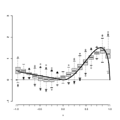
(a) Case 1

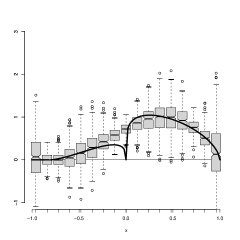
(b) Case 2

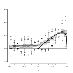
(c) Case 3

Figure 1: True mixture densities (solid line) and the box plots of the estimates. Number of replications $M=500$, sample size $n=1500$.

	$w$	$a_{*}$	$(p_{1},q_{1})$	$(p_{2},q_{2})$	$(p_{3},q_{3})$	$d$	$\alpha$
Case 1	0.8	0.95	(3.0, 1.5)	(2.0, 1.0)	–	0.25	0.5
Case 2	0.8	0.80	(1.2, 1.6)	(1.3, 2.5)	–	0.20	0.6
Case 3	0.8	0.90	–	–	(2.0, 1.2)	0.40	0.2

Table 1: Parameter values in cases 1–3.

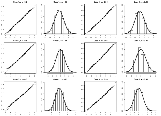
Figure 2: QQ plots and histograms of the estimates at points $x=-0.5$ and $x=0.96$. Number of replications $M=500$, sample size $n=1500$.

Box plots in Figure 1 show that $\hat{\varphi}_{n}$ approximates the mixture density well when $n$ is sufficiently large. However, when the sample size is relatively small it is difficult to estimate the mixture density of the shape as in cases 2–3. This can be explained by the construction of the estimator which assumes rather smooth form of the mixture density around zero. On the other hand, it is clear that the AR(1) parameter values which are close to zero does not affect the long memory property. For our purposes, an important fact is that the estimator correctly approximates the density at the neighborhood of $x=1$. This enables us to estimate the unknown (in real applications) parameter $d$ using a $\log$–$\log$ regression on periodogram at the neighborhood of this point (for example Geweke and Porter-Hudak or Whittle-type estimators).

Figure 2 supplements the earlier findings and shows that the distribution of estimator is approximately normal. QQ-plots and histograms are given for fixed values $x=-0.5$ and $x=0.96$ correspondingly. We use the same number of replications $M=500$ and sample size $n=1500$.

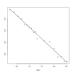
(a) Case 1, $x=-0.5$

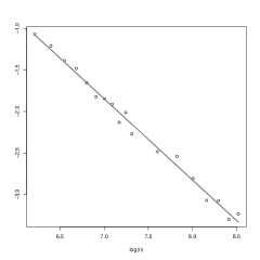
(b) Case 1, $x=0.96$

Figure 3: $\log$-$\log$ scale regression of the variance of $\hat{\varphi}_{n}(x)$ as a function of $n$. The variance is estimated using $M=500$ independent replications.

The last Monte-Carlo experiment aims to show that the decay rate of ${\rm Var}(\hat{\varphi}_{n}(x))$ is $n^{-\gamma}$ with $\gamma=1$. This ensures that the variance is decreasing fast enough. To do this, we calculate the $\log$–$\log$ regression of variance on the length of time series $n\in\{500,600,\dots,1400,1500,2000,\dots,5000\}$. Figure 3 demonstrates the corresponding parameter estimates at different points and shows that $\hat{\gamma}\approx 1$.

6 Appendix A. Proof of Example 2.1

By Corollary 3.1 in Celov et al., (2007), the mixture density $\varphi(x)$, $x\in[-a_{*},1]$ associated with $f(\lambda)$ (2.20) is given by equality (3.11), where $\varphi_{g}(x)\equiv\varphi_{g}(x;\kappa)$. Clearly, in this case, (3.11) can be rewritten in form (2.13) with

$$\psi(x)=\tilde{C}(\psi_{1}(x)+\psi_{2}(x)),$$ (6.1)

where $\tilde{C}=C_{1}(d)C_{2}(\kappa)C^{-1}_{*}$ is positive constant,

$$\psi_{1}(x) := x^{d-1}(1+x){\bf 1}_{(0,1]}(x)\int_{-a_{*}}^{0}\frac{|y|^{\kappa}}{(1-xy)(1-y/x)}\;\mathrm{d}y,$$ (6.2)

$$\psi_{2}(x) := |x|^{\kappa}(1-x)^{2d-1}{\bf 1}_{[-a_{*},0]}(x)\int_{0}^{1}\frac{y^{d-1}(1-y)^{1-2d}(1+y)}{(1-xy)(1-y/x)}\;\mathrm{d}y.$$ (6.3)

Denote by $F(a,b;c;x)$ a hypergeometric function

$$F(a,b;c;x)=\frac{\Gamma(c)}{\Gamma(b)\Gamma(c-b)}\int_{0}^{1}t^{b-1}(1-t)^{c-b-1}(1-tx)^{-a}\mathrm{d}t,$$

with $c>b>0$ if $x<1$ and, in addition, $c-a-b>0$ if $x=1$. Then the corresponding integrals in $\psi_{1}(x)$ and $\psi_{2}(x)$ can be rewritten as

$$\int_{-a_{*}}^{0}\frac{|y|^{\kappa}}{(1-xy)(1-y/x)}\;\mathrm{d}y,$$

$$= \frac{a_{*}^{\kappa+1}}{\kappa+1}\frac{x(F(1,\kappa+1;\kappa+2;-a_{*}x)-F(1,\kappa+1;\kappa+2;-a_{*}/x))}{1-x^{2}}$$

$$\sim \frac{a_{*}^{\kappa+1}}{\kappa+1}\ x,\ \ {\rm as}\ \ x\to 0+,$$

and

$$\int_{0}^{1}\frac{y^{d-1}(1-y)^{1-2d}(1+y)}{(1-xy)(1-y/x)}\;\mathrm{d}y$$

$$= \frac{\Gamma(d)\Gamma(2-2d)}{\Gamma(2-2d)}\frac{F(1,d;2-d;1/x)-xF(1,d;2-d;x)}{1-x}$$

$$\sim \Gamma(d)\Gamma(1-d)|x|^{d},\ \ {\rm as}\ \ x\to 0-,$$

where the last asymptotics follow from the well known properties of the hypergeometric functions (see Abramovitz and Stegun, (1965)).

Thus, from (6.2)–(6.3) we obtain that

$$\psi_{1}(x) \sim \frac{a_{*}^{\kappa+1}}{\kappa+1}\ x^{d},\ \ {\rm as}\ \ x\to 0+,$$ (6.4)

$$\psi_{2}(x) \sim \Gamma(d)\Gamma(1-d)|x|^{\kappa+d},\ \ {\rm as}\ \ x\to 0-.$$ (6.5)

(6.1) and relations (6.4)–(6.5) complete the proof. $\Box$

7 Appendix B. Proofs of lemmas 4.1–4.2

Proof of Lemma 4.1. By (4.6),

$$(1-x^{2})^{-\alpha}\eta_{n}(\lambda;x) = \sum_{k=0}^{K_{n}}G_{k}^{(\alpha)}(x)\sum_{j=0}^{k}g_{k,j}^{(\alpha)}(\mathrm{e}^{\mathrm{i}\lambda j}-\mathrm{e}^{\mathrm{i}\lambda(j+2)})$$

$$= (1-\mathrm{e}^{2\mathrm{i}\lambda})\sum_{k=0}^{K_{n}}G_{k}^{(\alpha)}(x)\sum_{j=0}^{k}g_{k,j}^{(\alpha)}\mathrm{e}^{\mathrm{i}\lambda j}$$

$$= (1-\mathrm{e}^{2\mathrm{i}\lambda})\sum_{k=0}^{K_{n}}G_{k}^{(\alpha)}(x)G_{k}^{(\alpha)}(\mathrm{e}^{\mathrm{i}\lambda}).$$

This and Lemma 7.1 below implies

$$(1-x^{2})^{-\alpha}|\eta_{n}(\lambda;x)| \leq C_{11}|\lambda|^{-(2\alpha-3)/4}\sum_{k=0}^{K_{n}}|G_{k}^{(\alpha)}(x)|(1+\sqrt{2})^{k}.$$ (7.1)

Now, using the fact that for all $-1<x<1$

$$|G_{k}^{(\alpha)}(x)|\leq\begin{cases}C_{12}(1-x^{2})^{-\frac{\alpha}{2}-\frac{1}{4}}&{\rm if}\ \ \alpha>-1/2\\ C_{12}&{\rm if}\ \ \alpha<-1/2,\ \alpha\neq-3/2,-5/2,\dots\end{cases}$$

(see inequality (7.33.6) in Szegö, (1967) and (3.9) in Leipus et al., (2006)) and (2.9), we get from (7.1)

$$(1-x^{2})^{-\alpha}|\eta_{n}(\lambda;x)| \leq C_{13}|\lambda|^{-(2\alpha-3)/4}(1+\sqrt{2})^{K_{n}}$$

$$= C_{13}|\lambda|^{-(2\alpha-3)/4}\mathrm{e}^{K_{n}\log(1+\sqrt{2})}$$

$$\leq C_{9}|\lambda|^{-(2\alpha-3)/4}n^{\gamma\log(1+\sqrt{2})}.$$

$\Box$

Lemma 7.1

For all $k\geq 0$, $\alpha>-1$, ($\alpha\neq-1/2$) and $0<|\lambda|<\pi$ it holds

$$|(1-\mathrm{e}^{2\mathrm{i}\lambda})G_{k}^{(\alpha)}(\mathrm{e}^{\mathrm{i}\lambda})|\leq C_{11}(1+\sqrt{2})^{k}|\lambda|^{-(2\alpha-3)/4},$$

where constant $C_{11}$ depends on $\alpha$.

Proof. Theorem 8.21.10 of Szegö, (1967) implies that for the usual (nonnormalized) Gegenbauer polynomials with $\alpha>-1$, $\alpha\neq-1/2$ it holds

$$C_{k}^{(\alpha+1/2)}(\mathrm{e}^{\mathrm{i}\lambda})=\frac{\Gamma(k+\alpha+\frac{1}{2})}{\Gamma(k+1)\Gamma(\alpha+\frac{1}{2})}\;z^{k}(1-z^{-2})^{-\alpha-1/2}+O(k^{\alpha-3/2}|z|^{k}),$$ (7.2)

where the complex numbers $w=\mathrm{e}^{\mathrm{i}\lambda}$ and $z$ are connected by the elementary conformal mapping

$$w=\frac{1}{2}(z+z^{-1}),\quad z=w+(w^{2}-1)^{1/2},$$ (7.3)

and $z$ satisfies $|z|>1$ (thus, $\lambda\neq 0,\pm\pi$).

Recall that the normalized Gegenbauer polynomials $G_{k}^{(\alpha)}(z)$ are linked to $C_{k}^{(\alpha+1/2)}(z)$ by equality

$$G_{k}^{(\alpha)}(z)=\gamma_{k}^{-1/2}C_{k}^{(\alpha+1/2)}(z),\ \textrm{where}\ \gamma_{k}=\frac{\pi}{2^{2\alpha}}\frac{\Gamma(k+2\alpha+1)}{(k+\alpha+\frac{1}{2})\Gamma^{2}(\alpha+\frac{1}{2})\Gamma(k+1)}.$$

Therefore, in terms of the normalized Gegenbauer polynomials, (7.2) reads as follows

$$G_{k}^{(\alpha)}(\mathrm{e}^{\mathrm{i}\lambda})=\frac{{\rm sgn}(\alpha+1/2)2^{\alpha}}{\pi^{1/2}}\ b_{k}z^{k}(1-z^{-2})^{-\alpha-1/2}+O(k^{-1}|z|^{k}),$$ (7.4)

where

$$b_{k}=\frac{(k+\alpha+1/2)^{1/2}\Gamma(k+\alpha+1/2)}{\Gamma^{1/2}(k+1)\Gamma^{1/2}(k+2\alpha+1)}\to 1\ \ {\rm as}\ \ k\to\infty.$$

From (7.3) we obtain for $w=\mathrm{e}^{\mathrm{i}\lambda}$

$$w^{2}-1=\frac{1}{4}z^{2}(1-z^{-2})^{2},$$

which together with (7.4) yields

$$(1-\mathrm{e}^{2\mathrm{i}\lambda})G_{k}^{(\alpha)}(\mathrm{e}^{\mathrm{i}\lambda})=-\frac{{\rm sgn}(\alpha+1/2)2^{\alpha}}{4\pi^{1/2}}\ b_{k}z^{k+2}(1-z^{-2})^{-\alpha+3/2}+O(k^{-1}|z|^{k}).$$

Since $|z|>1$ and $z^{2}-1=2(\mathrm{e}^{2\mathrm{i}\lambda}-1)+2\mathrm{e}^{3\mathrm{i}\lambda/2}(\mathrm{e}^{\mathrm{i}\lambda}-\mathrm{e}^{-\mathrm{i}\lambda})^{1/2}$, we have

$$|1-z^{-2}| \leq |z^{2}-1|$$ (7.5)

$$\leq 2|\mathrm{e}^{2\mathrm{i}\lambda}-1|+2|\mathrm{e}^{\mathrm{i}\lambda}-\mathrm{e}^{-\mathrm{i}\lambda}|^{1/2}$$

$$= 4|\sin\lambda|+2\sqrt{2}|\sin\lambda|^{1/2}$$

$$\leq (4+2\sqrt{2})|\lambda|^{1/2}.$$

So that, by (7.4)–(7.5),

$$|(1-\mathrm{e}^{2\mathrm{i}\lambda})G_{k}^{(\alpha)}(\mathrm{e}^{\mathrm{i}\lambda})|\leq C_{14}b_{k}|z|^{k}|\lambda|^{-(2\alpha-3)/4},$$ (7.6)

where $C_{14}=C_{14}(\alpha)$.

Finally, the straightforward verification shows that

$$\sup_{\lambda\in[-\pi,\pi]}|\mathrm{e}^{\mathrm{i}\lambda}+(\mathrm{e}^{2\mathrm{i}\lambda}-1)^{1/2}|=1+\sqrt{2}.$$

This completes the proof of lemma. $\Box$

Proof of Lemma 4.2. Using (4.2), (4.6) rewrite the coefficients of $E_{n}$

$$e_{n}(t-s)=(1-x^{2})^{\alpha}\sum_{k=0}^{K_{n}}G_{k}^{(\alpha)}(x)\sum_{j=0}^{k}g_{k,j}^{(\alpha)}\int_{-\pi}^{\pi}f(\lambda)(\mathrm{e}^{\mathrm{i}\lambda(t-s+j)}-\mathrm{e}^{\mathrm{i}\lambda(t-s+j+2)})\mathrm{d}\lambda.$$

Using the expression of the covariance function of an aggregated process, we have for $t-s+j\geq 0$

$$\int_{-\pi}^{\pi}f(\lambda)(\mathrm{e}^{\mathrm{i}\lambda(t-s+j)}-\mathrm{e}^{\mathrm{i}\lambda(t-s+j+2)})\mathrm{d}\lambda = \sigma(t-s+j)-\sigma(t-s+j+2)$$

$$= \sigma_{\varepsilon}^{2}\int_{-1}^{1}y^{t-s+j}\varphi(y)\mathrm{d}y.$$

Thus, assuming $\sigma_{\varepsilon}^{2}=1$, for $t-s\geq 0$ we have

$$e_{n}(t-s) = (1-x^{2})^{\alpha}\sum_{k=0}^{K_{n}}G_{k}^{(\alpha)}(x)\sum_{j=0}^{k}g_{k,j}^{(\alpha)}\int_{-1}^{1}y^{t-s+j}\varphi(y)\mathrm{d}y$$

$$= (1-x^{2})^{\alpha}\sum_{k=0}^{K_{n}}G_{k}^{(\alpha)}(x)\int_{-1}^{1}y^{t-s}\varphi(y)\sum_{j=0}^{k}g_{k,j}^{(\alpha)}y^{j}\mathrm{d}y$$

$$= (1-x^{2})^{\alpha}\sum_{k=0}^{K_{n}}G_{k}^{(\alpha)}(x)\int_{-1}^{1}y^{t-s}\varphi(y)G_{k}^{(\alpha)}(y)\mathrm{d}y.$$

Integral $\int_{-1}^{1}y^{m}\varphi(y)G_{k}^{(\alpha)}(y)\mathrm{d}y$ ($m$ is a nonnegative integer), appearing in the last expression is nothing else but the $k$th coefficient, $\psi_{m,k}$, in the $\alpha$-Gegenbauer expansion of the function

$$\psi_{m}(x)=\frac{x^{m}\varphi(x)}{(1-x^{2})^{\alpha}},$$ (7.7)

which obviously satisfies $\psi_{m}\in L^{2}(w^{(\alpha)})$. Therefore,

$$e_{n}(t-s) = (1-x^{2})^{\alpha}\sum_{k=0}^{K_{n}}G_{k}^{(\alpha)}(x)\psi_{|t-s|,k}$$

$$= (1-x^{2})^{\alpha}\bigg{(}\psi_{|t-s|}(x)-\sum_{k=K_{n}+1}^{\infty}G_{k}^{(\alpha)}(x)\psi_{|t-s|,k}\bigg{)}$$

and, denoting $R_{n}(m):=\sum_{k=K_{n}+1}^{\infty}G_{k}^{(\alpha)}(x)\psi_{|m|,k}$, $|m|<n$, we have

$$(1-x^{2})^{-2\alpha}\|E_{n}\|^{2} = \sum_{|m|<n}(n-|m|)\bigg{(}\psi_{|m|}(x)-\sum_{k=K_{n}+1}^{\infty}G_{k}^{(\alpha)}(x)\psi_{m,k}\bigg{)}^{2}$$

$$= \sum_{|m|<n}(n-|m|)\psi^{2}_{|m|}(x)-2\sum_{|m|<n}(n-|m|)\psi_{|m|}(x)R_{n}(m)$$

$$+\sum_{|m|<n}(n-|m|)R^{2}_{n}(m)=:A_{1,n}-2A_{2,n}+A_{3,n}.$$

Now, we prove that, as $n\to\infty$,

$$A_{1,n}\sim C_{15}n,$$ (7.8)

where $C_{15}=C_{15}(x)>0$ is some positive constant, and

$$A_{2,n}=o(n).$$ (7.9)

Since the last term $A_{3,n}$ is nonnegative by construction, this will prove (4.9).

At points $x$ where $\varphi(x)\neq 0$ we have

$$A_{1,n} = \frac{\varphi^{2}(x)}{(1-x^{2})^{2\alpha}}\sum_{|m|<n}(n-|m|)x^{2|m|}$$

$$\sim n\;\frac{\varphi^{2}(x)(1+x^{2})}{(1-x^{2})^{2\alpha+1}},\ \ {\rm as}\ \ n\to\infty,$$

which gives (7.8). Consider term $A_{2,n}$. By (7.7),

$$A_{2,n} = \sum_{|m|<n}(n-|m|)\psi_{|m|}(x)\sum_{k=K_{n}+1}^{\infty}G_{k}^{(\alpha)}(x)\psi_{|m|,k}$$

$$= \frac{\varphi(x)}{(1-x^{2})^{\alpha}}\sum_{k=K_{n}+1}^{\infty}G_{j}^{(\alpha)}(x)\int_{-1}^{1}\varphi(y)G_{k}^{(\alpha)}(y)\sum_{|m|<n}(n-|m|)(xy)^{|m|}\mathrm{d}y$$

$$= \frac{\varphi(x)}{(1-x^{2})^{\alpha}}\;(B_{1,n}-B_{2,n}-B_{3,n}),$$

where

$$B_{1,n} := n\sum_{k=K_{n}+1}^{\infty}G_{j}^{(\alpha)}(x)\int_{-1}^{1}\varphi(y)G_{k}^{(\alpha)}(y)\sum_{m=-\infty}^{\infty}(xy)^{|m|}\mathrm{d}y,$$

$$= n\sum_{k=K_{n}+1}^{\infty}G_{j}^{(\alpha)}(x)\int_{-1}^{1}\varphi(y)G_{k}^{(\alpha)}(y)\frac{1+xy}{1-xy}\;\mathrm{d}y,$$

$$B_{2,n} := \sum_{k=K_{n}+1}^{\infty}G_{j}^{(\alpha)}(x)\int_{-1}^{1}\varphi(y)G_{k}^{(\alpha)}(y)\sum_{|m|<n}|m|(xy)^{|m|}\mathrm{d}y,$$

$$B_{3,n} := n\sum_{k=K_{n}+1}^{\infty}G_{j}^{(\alpha)}(x)\int_{-1}^{1}\varphi(y)G_{k}^{(\alpha)}(y)\sum_{|m|\geq n}(xy)^{|m|}\mathrm{d}y.$$

Since, by (2.6),

$$\tilde{\varphi}_{x}(y)\equiv\frac{\varphi(y)}{(1-y^{2})^{\alpha}}\frac{1+xy}{1-xy}$$

satisfies $\tilde{\varphi}_{x}\in L^{2}(w^{(\alpha)})$ and $K_{n}\to\infty$, the sum $\sum_{k=K_{n}+1}^{\infty}$ in $B_{1,n}$ vanishes (as the tail of the convergent series). So that, $B_{1,n}=o(n)$ and, similarly, $B_{3,n}=o(n)$.

Finally,

$$B_{2,n} \sim \sum_{k=K_{n}+1}^{\infty}G_{j}^{(\alpha)}(x)\int_{-1}^{1}\varphi(y)G_{k}^{(\alpha)}(y)\;\frac{2xy}{(1-xy)^{2}}\;\mathrm{d}y=o(1)$$

using the similar argument as in the case of term $B_{1,n}$. This completes the proof of (7.9) and of the lemma. $\Box$

References

Abramovitz and Stegun, (1965)
Abramovitz, M. and Stegun, I. (1965).
Handbook of Mathematical Functions with Formulas,
Graphs, and Mathematical Tables.
New York, Dover Publications.
Anderson, (1971)
Anderson, T. (1971).
The Statistical Analysis of Time Series.
Wiley Series in Probability and Mathematical Statistics, New York.