Central limit theorem for Hotelling’s $T^{2}$ statistic under large dimension

Abstract

In this paper we prove the central limit theorem for Hotelling’s $T^{2}$ statistic when the dimension of the random vectors is proportional to the sample size.

and

t1Supported in part by Grant M58110052 at the Nanyang Technological University.

t2Supported in part by Grant R-155-000-106-112 at the National University of Singapore.

1 Introduction and main results

Since the famous Marčenko and Pastur law was found in MP , the theory of large sample covariance matrices has been further developed. Among others, we mention Jonsson Jon , Yin y1 , Silverstein s1 , Watcher watch , Yin, Bai and Krishanaiah y2 . Lately, Johnstone john discovered the law of the largest eigenvalue of the Wishart matrix, Bai and Silverstein b2 established the central limit theorems (CLT) of linear spectral statistics and Bai, Miao and Pan b1 derived CLT for functionals of the eigenvalues and eigenvectors. We also refer to johan , ss , Di for CLT on linear statistics of eigenvalues of other classes of random matrices.

The sample covariance matrix is defined by

$$\bolds{\mathcal{S}}=\frac{1}{n}\sum_{j=1}^{n}({\mathbf{s}}_{j}-\bar{\mathbf{s}})({\mathbf{s}}_{j}-\bar{\mathbf{s}})^{T},$$

where $\bar{\mathbf{s}}=n^{-1}\sum_{j=1}^{n}{\mathbf{s}}_{j}$ and ${\mathbf{s}}_{j}=(X_{1j},\ldots,X_{pj})^{T}$. Here {$X_{ij}$}, $i,j=\cdots,$ is a double array of independent and identically distributed (i.i.d.) real r.v.’s with $EX_{11}=0$ and $EX_{11}^{2}=1$. However, in the large random matrices theory (RMT) the commonly used sample covariance matrix is

$$\mathbf{S}=\frac{1}{n}\sum_{j=1}^{n}{\mathbf{s}}_{j}{\mathbf{s}}_{j}^{T}=\frac{1}{n}\mathbf{X}_{n}\mathbf{X}_{n}^{T},$$

where $\mathbf{X}_{n}=({\mathbf{s}}_{1},\ldots,{\mathbf{s}}_{n})$.

Note that $\bolds{\mathcal{S}}=\mathbf{S}-\bar{\mathbf{s}}\bar{\mathbf{s}}^{T}$ and thus, by the rank inequality, there is no difference when one is only concerned with the limiting empirical spectral distribution (ESD) of the eigenvalues in large random matrices. Therefore, the limiting ESD of $\bolds{\mathcal{S}}$ is Marčenko and Pastur’s law $F_{c}(x)$ (see Jon and MP ) when $\lim\frac{p}{n}=c>0$ which has a density function

$$p_{c}(x)=\cases{(2\pi cx)^{-1}\sqrt{(b-x)(x-a)},&\quad$a\leq x\leq b$,\cr 0,&\quad otherwise,}$$

and has point mass $1-c^{-1}$ at the origin if $c>1$, where $a=(1-\sqrt{c})^{2}$ and $b=(1+\sqrt{c})^{2}$. The Stieljes transform $m(z)$ of $F_{c}(x)$ satisfies the equation (see s3 )

$$m(z)=\frac{1}{1-c-czm(z)-z},$$ (1)

where the Stieljes transform for any function $G(x)$ is defined by

$$m_{G}(z)=\int\frac{1}{\lambda-z}\,dG(\lambda),\qquad z\in{\mathbb{C}}^{+}\equiv\{z\in{\mathbb{C}},v=\Im z>0\}.$$

Observe that the spectra of $n^{-1}\mathbf{X}_{n}\mathbf{X}_{n}^{T}$ and $n^{-1}\mathbf{X}_{n}^{T}\mathbf{X}_{n}$ are identical except for zero eigenvalues. This leads to the equality

$$\underline{m}_{n}^{\mathbf{S}}(z)=-\frac{1-p/n}{z}+\frac{p}{n}m_{n}^{\mathbf{S}}(z)$$ (2)

and therefore,

$$z=-\frac{1}{\underline{m}(z)}+\frac{c}{1+\underline{m}(z)},$$ (3)

where $m_{n}^{\mathbf{S}}(z)$ and $\underline{m}_{n}^{\mathbf{S}}(z)$ denote, respectively, the Stieljes transform of the ESD of $n^{-1}\mathbf{X}_{n}\mathbf{X}_{n}^{T}$ and $n^{-1}\mathbf{X}_{n}^{T}\mathbf{X}_{n}$ and, correspondingly, $\underline{m}(z)$ is the limit of $\underline{m}_{n}^{\mathbf{S}}(z)$.

Sample covariance matrices are also of essential importance in multivariate statistical analysis because many test statistics involve their eigenvalues and/or eigenvectors. The typical example is $T^{2}$ statistic which was proposed by Hotelling h . We refer to a1 and leh for various uses of the $T^{2}$ statistic.

The $T^{2}$ statistic, which is the origin of multivariate linear hypothesis tests and the associated confidence sets, is defined by

$$T^{2}=n(\bar{\mathbf{s}}-\bolds{\mu}_{0})^{T}\bolds{\mathcal{S}}^{-1}(\bar{\mathbf{s}}-\bolds{\mu}_{0}),$$ (4)

whose distribution is invariant if each ${\mathbf{s}}_{j}$ is replaced by $\bolds\Sigma^{1/2}{\mathbf{s}}_{j}$ with $\bolds\Sigma$ any nonsingular $p$ by $p$ matrix when $\bolds{\mu}_{0}=0$. If $\{{\mathbf{s}}_{1},\ldots,{\mathbf{s}}_{n}\}$ is a sample from the $p$-dimensional population $N(\bolds{\mu},\bolds\Sigma)$, then $[T^{2}/(n-1)][(n-p)/p]$ follows a noncentral $F$ distribution and moreover, the $F$ distribution is central if $\bolds{\mu}=\bolds{\mu}_{0}$. When $p$ is fixed, the limiting distribution of $T^{2}$ for $\bolds{\mu}=\bolds{\mu}_{0}$ is the $\chi^{2}$-distribution even if the parent distribution is not normal.

In the recent three or four decades in many research areas, including signal processing, network security, image processing, genetics, stock marketing and other economic problems, people are interested in the case where $p$ is quite large or proportional to the sample size. Thus, it will be desirable if one can obtain the asymptotic distribution of the famous Hotelling $T^{2}$ statistic when the dimension of the random vectors is proportional to the sample size. It is the aim of this work. In addition, we would like to point out that some discussions about the two-sample $T^{2}$ statistic under the assumption that the underlying r.v.’s are normal were presented in b5 .

The main results are presented in the following theorems.

Theorem 1

Suppose that:

[(2)]

for each $n$ $X_{ij}=X_{ij}^{n},i,j=1,2,\ldots,$ are i.i.d. real r.v.’s with $EX_{11}=\mu,EX_{11}^{2}=1$ and $EX_{11}^{4}<\infty$.

$p\leq n,c_{n}=p/n\to c\in(0,1)$ as $n\to\infty$.

Then, when $\bolds{\mu}_{0}=(\mu,\ldots,\mu)^{T}$,

$$\frac{\sqrt{n}}{\sqrt{2c_{n}(1-c_{n})^{-3}}}\biggl{(}\frac{T^{2}}{n}-c_{n}(1-c_{n})^{-1}\biggr{)}\stackrel{{\scriptstyle D}}{{\longrightarrow}}N(0,1),$$

where $F_{c_{n}}(x)$ denotes $F_{c}(x)$ by substituting $c_{n}$ for $c$.

Remark 1

When $X_{ij}\sim N(0,1)$, it is well known that $(n-p)T^{2}/(np)$ follows $F$ distribution with degrees of freedom $p$ and $n-p$, respectively. As $n\to\infty$ and $p/n\to c$, it follows from strong law of large numbers and CLT that

$$\frac{(n-p)T^{2}/(np)-1}{\sqrt{2/p+2/(n-p)}}\longrightarrow N(0,1).$$

This is consistent with Theorem 1.

Remark 2

Since $\int x^{-1}\,dF_{c}(x)=(1-c)^{-1}$ and $\int x^{-2}\,dF_{c}(x)=(1-c)^{-3}$ which are derived through differentiating the following identity [the Stieljes transform $m(z)$ of $F_{c}(x)$],

$$\int(x-z)^{-1}p_{c}(x)\,dx=\frac{-(z+c-1)+(z+c-1)\sqrt{1-4zc(z+c-1)^{-2}}}{2cz},$$

we actually prove that

$$\frac{\sqrt{n}}{\sqrt{2c_{n}\int x^{-2}\,dF_{c_{n}}(x)}}\biggl{(}\frac{T^{2}}{n}-c_{n}\int\frac{dF_{c_{n}}(x)}{x}\biggr{)}\stackrel{{\scriptstyle D}}{{\longrightarrow}}N(0,1).$$

One typical application of Theorem 1 lies in making inference on the large-dimensional mean vector of the multivariate model

$$\mathbf{Z}_{j}=\Gamma{\mathbf{s}}_{j}+\bolds{\mu},\qquad E{\mathbf{s}}_{j}=0,\qquad j=1,\ldots,n,$$

where $\Gamma$ is an $m$ by $p$ matrix, $m\leq p$. This model means that each $\mathbf{Z}_{j}$ is a linear transformation of some $p$-variate random vector ${\mathbf{s}}_{j}$. It can generate a rich collection of $\mathbf{Z}_{j}$ from ${\mathbf{s}}_{j}$ with the given covariance matrix $\bolds\Sigma=\Gamma\Gamma^{T}$. Most important, it includes the multivariate normal model.

We will prove Theorem 1 by establishing Theorem 2 which presents asymptotic distributions of random quadratic forms involving sample means and sample covariance matrices.

For any analytic function $f(\cdot)$, define

$$f(\bolds{\mathcal{S}})=\mathbf{U}^{T}\operatorname{diag}(f(\lambda_{1}),\ldots,f(\lambda_{p}))\mathbf{U},$$

where $\mathbf{U}^{T}\operatorname{diag}(\lambda_{1},\ldots,\lambda_{p})\mathbf{U}$ denotes the spectral decomposition of the matrix $\bolds{\mathcal{S}}$.

Theorem 2

In addition to the assumption $(1)$ of Theorem 1, suppose that $c_{n}=p/n\to c>0$, $EX_{11}=0$, $g(x)$ is a function with a continuous first derivative in a neighborhood of $c$ and $f(x)$ is analytic on an open region containing the interval

$$\bigl{[}I_{(0,1)}(c)\bigl{(}1-\sqrt{c}\bigr{)}^{2},\bigl{(}1+\sqrt{c}\bigr{)}^{2}\bigr{]}.$$ (5)

Then,

$$\biggl{(}\sqrt{n}\biggl{[}\frac{\bar{\mathbf{s}}^{T}f(\bolds{\mathcal{S}})\bar{\mathbf{s}}}{\|\bar{\mathbf{s}}\|^{2}}-\int f(x)\,dF_{c_{n}}(x)\biggr{]},\sqrt{n}\bigl{(}g(\bar{\mathbf{s}}^{T}\bar{\mathbf{s}})-g(c_{n})\bigr{)}\biggr{)}\stackrel{{\scriptstyle D}}{{\longrightarrow}}(X,Y),$$

where $Y\sim N(0,2c(g^{\prime}(c))^{2})$, which is independent of $X$, a Gaussian r.v. with $EX=0$ and

$$\operatorname{Var}(X)=\frac{2}{c}\biggl{(}\int f^{2}(x)\,dF_{c}(x)-\biggl{(}\int f(x)\,dF_{c}(x)\biggr{)}^{2}\biggr{)}.$$ (6)

Remark 3

Let $\mathbf{x}_{n}=(x_{n1},\ldots,x_{np})^{T}\in\mathbb{R}^{p}$, $\|\mathbf{x}_{n}\|=1$ where $\|\cdot\|$ denotes the Euclidean norm. Note that, when $\max_{i}x_{ni}\rightarrow 0$ (see p2 , (1.16), or s2 ),

$$\sqrt{n}\biggl{[}\mathbf{x}_{n}^{T}f(\mathbf{S})\mathbf{x}_{n}-\int f(x)\,dF_{c_{n}}(x)\biggr{]}\stackrel{{\scriptstyle D}}{{\longrightarrow}}X.$$ (7)

This suggests that $\bar{\mathbf{s}}/\|\bar{\mathbf{s}}\|$ can be viewed as a fixed unit vector $\mathbf{x}_{n}$ when dealing with $\bar{\mathbf{s}}^{T}f(\bolds{\mathcal{S}})\bar{\mathbf{s}}/\|\bar{\mathbf{s}}\|^{2}$ even if $\bar{\mathbf{s}}$ is not independent of $\bolds{\mathcal{S}}$.

Theorem 2 relies on Lemma 1 below which deals with the asymptotic joint distribution of

$$X_{n}(z)=\sqrt{n}\biggl{[}\frac{\bar{\mathbf{s}}^{T}(\bolds{\mathcal{S}}-z\mathbf{I})^{-1}\bar{\mathbf{s}}}{\|\bar{\mathbf{s}}\|^{2}}-m_{n}(z)\biggr{]},\qquad Y_{n}=\sqrt{n}\bigl{(}g(\bar{\mathbf{s}}^{T}\bar{\mathbf{s}})-g(c_{n})\bigr{)},$$

where $m_{n}(z)=\int(x-z)^{-1}\,dF_{c_{n}}(x)$. The stochastic process $X_{n}(z)$ is defined on a contour $\mathcal{C}$, given below. Let $v_{0}>0$ be arbitrary and set $\mathcal{C}_{u}=\{u+iv_{0},u\in[u_{l},u_{r}]\},$ where $u_{l}$ is any negative number if the left endpoint of (5) is zero, otherwise $u_{l}$ is any positive number smaller than the left endpoint of (5) and $u_{r}$ any number larger than the right endpoint of (5). Then define

$$\mathcal{C}^{+}=\{u_{l}+iv\dvtx v\in[0,v_{0}]\}\cup\mathcal{C}_{u}\cup\{u_{r}+iv\dvtx v\in[0,v_{0}]\}$$

and let $\mathcal{C}^{-}$ be the symmetric part of $\mathcal{C}^{+}$ about the real axis. Then set $\mathcal{C}=\mathcal{C}^{+}\cup\mathcal{C}^{-}$. See Figures 1 and 2 for a picture of the contour $\mathcal{C}$ when $c<1$ and $c\geq 1$, respectively.

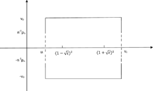
Figure 1: Contour $\mathcal{C}$ when $c<1$.

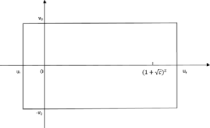
Figure 2: Contour $\mathcal{C}$ when $c\geq 1$.

Let $\mathbf{A}^{-1}(z)=(\mathbf{S}-zI)^{-1}$. Since it is difficult to control the spectral norm of $(\bolds{\mathcal{S}}-z\mathbf{I})^{-1}$ or $\mathbf{A}^{-1}(z)$ on the whole contour $\mathcal{C}$, especially for $v=0$, we further define $\hat{X}_{n}(z)$, a truncated version of $X_{n}(z)$, as in b2 . Select a sequence of positive numbers $\rho_{n}$ satisfying for some $\beta\in(0,1)$,

$$\rho_{n}\downarrow 0,\qquad\rho_{n}\geq n^{-\beta}.$$ (8)

Let

$$\mathcal{C}_{l}=\cases{\{u_{l}+iv\dvtx v\in[n^{-1}\rho_{n},v_{0}]\},&\quad if $u_{l}>0$,\cr\{u_{l}+iv\dvtx v\in[0,v_{0}]\},&\quad if $u_{l}<0$,}$$

and

$$\mathcal{C}_{r}=\{u_{r}+iv\dvtx v\in[n^{-1}\rho_{n},v_{0}]\}.$$

Write $\mathcal{C}_{n}^{+}=\mathcal{C}_{l}\cup\mathcal{C}_{u}\cup\mathcal{C}_{r}$. We can now define the truncated process for $z=u+iv\in\mathcal{C}$ by

$$\hat{X}_{n}(z)=\cases{X_{n}(z),\qquad\mbox{if $z\in\mathcal{C}_{n}^{+}\cup\mathcal{C}_{n}^{-}$},\cr\displaystyle\frac{nv+\rho_{n}}{2\rho_{n}}X_{n}(z_{r1})+\frac{\rho_{n}-nv}{2\rho_{n}}X_{n}(z_{r2}),\cr\hskip 1.5pt\phantom{X_{n}(z),}\qquad\mbox{if $u=u_{r},v\in[-n^{-1}\rho_{n},n^{-1}\rho_{n}]$},\cr\displaystyle\frac{nv+\rho_{n}}{2\rho_{n}}X_{n}(z_{l1})+\frac{\rho_{n}-nv}{2\rho_{n}}X_{n}(z_{l2}),\cr\hskip 1.5pt\phantom{X_{n}(z),}\qquad\mbox{if $u=u_{l}>0,v\in[-n^{-1}\rho_{n},n^{-1}\rho_{n}]$},}$$ (9)

where $z_{r1}=u_{r}+in^{-1}\rho_{n},z_{r2}=u_{r}-in^{-1}\rho_{n},z_{l1}=u_{l}+in^{-1}\rho_{n},z_{l2}=u_{l}-in^{-1}\rho_{n}$ and $\mathcal{C}_{n}^{-}$ denotes the symmetric part of $\mathcal{C}_{n}^{+}$ about the real axis. A picture of $\mathcal{C}_{n}^{+}\cup\mathcal{C}_{n}^{-}$ is the rectangle in Figure 1 with the dash line removed. The advantage of $\hat{X}_{n}(z)$ over $X_{n}(z)$ is that the spectral norm of $\mathbf{A}^{-1}(z)$ involved in $\hat{X}_{n}(z)$ may be well controlled on the contour $\mathcal{C}$. Indeed, loosely speaking, all eigenvalues of $\mathbf{S}$ are located inside the interval (5) with a high probability. Therefore, the spectral norm of $\mathbf{A}^{-1}(z)$ corresponding to this case is bounded on $\mathcal{C}$. If some eigenvalues run outside of the interval (5) then, at least, we will still have an upper bound $n\rho_{n}^{-1}$ for the spectral norm of $\mathbf{A}^{-1}(z)$ on $\mathcal{C}$. But, the probability that some eigenvalues run outside of the interval (5) is very small, which can offset $n\rho_{n}^{-1}$ and even more. This is crucial to establish tightness of $\hat{X}_{n}(z)$ on the contour $\mathcal{C}$. On the other hand, such a truncation does not change the weak limit given in Theorem 2 because the truncation has been made only at the intervals of the length $2\rho_{n}/n$.

Note that $\hat{X}_{n}(z)$ may be viewed as a random element in the metric space $C(\mathcal{C},\mathbb{R}^{2})$ of continuous functions from $\mathcal{C}$ to $\mathbb{R}^{2}$. We are now in a position to state Lemma 1.

Lemma 1

Under the assumptions of Theorem 2, we have for $z\in\mathcal{C}$,

$$(\hat{X}_{n}(z),Y_{n})\stackrel{{\scriptstyle D}}{{\longrightarrow}}(X(z),Y),$$

where $Y\sim N(0,2c(g^{\prime}(c))^{2})$, which is independent of $X(z)$, a Gaussian stochastic process with mean zero and covariance function $\operatorname{Cov}(X(z_{1}),X(z_{2}))$ equal to

$$\quad\frac{2}{cz_{1}z_{2}[(1+\underline{m}(z_{1}))(1+\underline{m}(z_{2}))-c\underline{m}(z_{1})\underline{m}(z_{2})]}-\frac{2m(z_{1})m(z_{2})}{c}.$$ (10)

Remark 4

Also, note that $X(z)$ is exactly the weak limit of the stochastic process $\sqrt{n}(\mathbf{x}_{n}^{T}(\mathbf{S}-z\mathbf{I})^{-1})\mathbf{x}_{n}-m_{n}(z))$ when $\max_{i}x_{ni}\rightarrow 0$, whose covariance function is

$$\operatorname{Cov}(X(z_{1}),X(z_{2}))=\frac{2(z_{2}\underline{m}(z_{2})-z_{1}\underline{m}(z_{1}))^{2}}{c^{2}z_{1}z_{2}(z_{1}-z_{2})(\underline{m}(z_{1})-\underline{m}(z_{2}))}$$

(see b1 and p2 ).

We conclude this section by presenting the structure of this work. In Section 2, we present a simulation study to identify when the asymptotic normality “kicks in.” Then we turn to the proof. To transfer Lemma 1 to Theorem 2 we introduce a new empirical distribution function

$$F_{2}^{\mathbf{S}}(x)=\sum_{i=1}^{p}t_{i}^{2}I(\lambda_{i}\leq x),$$ (11)

where $\mathbf{t}=(t_{1},\ldots,t_{n})^{T}=\mathbf{U}\bar{\mathbf{s}}/\|\bar{\mathbf{s}}\|$ and $\mathbf{U}$ is the eigenvector matrix of $\mathcal{S}$. It turns out that $F_{2}^{\mathbf{S}}(x)$ and the ESD of $\mathbf{S}$ have the same limit, that is, $F_{2}^{\mathbf{S}}(x)\stackrel{{\scriptstyle\mathrm{i.p.}}}{{\longrightarrow}}F_{c}(x)$. Thus, by analyticity of $f(x)$, $\bar{\mathbf{s}}^{T}f(\bolds{\mathcal{S}})\bar{\mathbf{s}}/\|\bar{\mathbf{s}}\|^{2}$ in Theorem 2 is transferred to the Stieljes transform of $F_{2}^{\mathbf{S}}(x)$, $\bar{\mathbf{s}}^{T}(\bolds{\mathcal{S}}-z\mathbf{I})^{-1}\bar{\mathbf{s}}/\|\bar{\mathbf{s}}\|^{2}$. Moreover, note that

$$\frac{\bar{\mathbf{s}}^{T}\mathbf{A}^{-1}(z)\bar{\mathbf{s}}}{1-\bar{\mathbf{s}}^{T}\mathbf{A}^{-1}(z)\bar{\mathbf{s}}}=\bar{\mathbf{s}}^{T}(\bolds{\mathcal{S}}-z\mathbf{I})^{-1}\bar{\mathbf{s}}.$$ (12)

Indeed, this is from the identity (see s3 , (2.1))

$$\mathbf{r}^{T}(\mathbf{B}+a\mathbf{r}\mathbf{r}^{T})^{-1}=\frac{r^{T}\mathbf{B}^{-1}}{1+a\mathbf{r}^{T}\mathbf{B}^{-1}\mathbf{r}},$$ (13)

where $\mathbf{B}$ and $\mathbf{B}+a\mathbf{r}\mathbf{r}^{T}$ are both invertible, $\mathbf{r}\in\mathbb{R}^{p}$ and $a\in\mathbb{R}$. The stochastic process $X_{n}(z)$ in Lemma 1 is then transferred to the stochastic process $M_{n}(z)$, where

$$M_{n}(z)=\sqrt{n}\biggl{(}\bar{\mathbf{s}}^{T}\mathbf{A}^{-1}(z)\bar{\mathbf{s}}-\frac{c_{n}m_{n}(z)}{1+c_{n}m_{n}(z)}\biggr{)}.$$

The convergence of the stochastic process $M_{n}(z)$ is given in Sections 3 and 4. The proofs of Theorems 1 and 2, Lemma 1 and Remark 4 are included in Section 5. The last section picks up the truncation of the underlying r.v.’s and some useful lemmas. At this point we would like to point out that both this paper and b2 deal with Stieljes transform of random variables of interest and use martingale method to establish CLT. But the random variable of interest in this paper is a kind of random quadratic forms while b2 is concerned with the trace of random matrices.

Throughout this paper, to save notation, $\mathfrak{M}$ may denote different constants on different occasions.

2 Simulation study

In this section, we provide a simulation study to investigate the performance of normal approximations in Theorem 1. We consider three different populations, the standard normal distribution, the exponential distribution with parameter 1 and the Poisson distribution with parameter 1. From each population we generate 5000 samples of order $100\times 200$, $200\times 400$ and $400\times 800$ matrices, respectively, by routines in R. Each $p\times n$ matrix can be regarded as a collection of $n$ observations of $p$-dimensional vectors ${\mathbf{s}}$, so we can calculate $T^{2}$ for each matrix. Based on 5000 samples, we have 5000 observed $T^{2}$ which give us an estimator of the probability

$$P\biggl{(}\frac{\sqrt{n}}{\sqrt{2c_{n}(1-c_{n})^{-3}}}\biggl{(}\frac{T^{2}}{n}-c_{n}(1-c_{n})^{-1}\biggr{)}\leq x\biggr{)}$$

by

$$5000^{-1}\sum I\biggl{(}\frac{\sqrt{n}}{\sqrt{2c_{n}(1-c_{n})^{-3}}}\biggl{(}\frac{T^{2}}{n}-c_{n}(1-c_{n})^{-1}\biggr{)}\leq x\biggr{)}.$$

In Figures 3–11, there are nine curves. In each figure the horizontal axis means theoretical quantiles of the standard normal distribution and the vertical axis indicates sample quantiles of the normalized Hotelling’s $T^{2}$ statistics. Every curve represents the quantile-quantile plot for each sampled matrix. From these pictures we see that the quantiles of $T^{2}$ get closer to the standard normal one as the sample size and the dimension increase. Actually, when $p=100$ and $n=200$, normal distributions already “kick in.”

Figure 3: Q–Q plot for normal data when $p=100$.

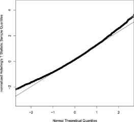
Figure 4: Q–Q plot for normal data when $p=200$.

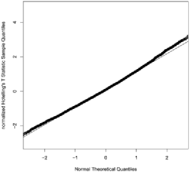
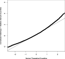
Figure 5: Q–Q plot for normal data when $p=400$.

Figure 6: Q–Q plot for exponential data when $p=100$.

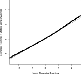
Figure 7: Q–Q plot for exponential data when $p=200$.

Figure 8: Q–Q plot for exponential data when $p=400$.

Figure 9: Q–Q plot for Poisson data when $p=100$.

Figure 10: Q–Q plot for Poisson data when $p=200$.

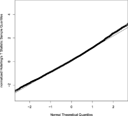
Figure 11: Q–Q plot for Poisson data when $p=400$.

3 Weak convergence of the finite-dimensional distributions

For $z\in\mathcal{C}_{n}^{+}$, let $M_{n}(z)=M_{n}^{(1)}(z)+M_{n}^{(2)}(z)$, where

$$M_{n}^{(1)}(z)=\sqrt{n}\bigl{(}\bar{\mathbf{s}}^{T}\mathbf{A}^{-1}(z)\bar{\mathbf{s}}-E\bar{\mathbf{s}}^{T}\mathbf{A}^{-1}(z)\bar{\mathbf{s}}\bigr{)}$$

and

$$M_{n}^{(2)}(z)=\sqrt{n}\biggl{(}E\bar{\mathbf{s}}^{T}\mathbf{A}^{-1}(z)\bar{\mathbf{s}}-\frac{c_{n}m_{n}(z)}{1+c_{n}m_{n}(z)}\biggr{)}.$$

In this section the aim is to prove that for any positive integer $r$ and complex numbers $a_{1},\ldots,a_{r}$,

$$\sum_{i=1}^{r}a_{i}M_{n}^{(1)}(z_{i}),\qquad\Im z_{i}\neq 0,$$

converges in distribution to a Gaussian r.v. and to derive the asymptotic covariance function. Before proceeding, r.v.’s need to be truncated. However, we shall postpone the truncation of r.v.’s until the last section. As a consequence of Lemma 7, we assume that the underlying r.v.’s satisfy

$$\quad|X_{ij}|\leq\varepsilon_{n}\sqrt{n},\qquad EX_{11}=0,\qquad E|X_{11}|^{2}=1,\qquad E|X_{11}|^{4}<\infty,$$ (14)

where $\varepsilon_{n}$ is a positive sequence which converges to zero as $n$ goes to infinity.

3.1 Outline of the argument

The underlying idea is to write $M_{n}^{(1)}(z)$ as a sum of martingale difference sequences and to apply Lemma 3, CLT for martingale. Define the $\sigma$-field ${\mathcal{F}}_{j}=\sigma({\mathbf{s}}_{1},\ldots,{\mathbf{s}}_{j})$ and let $E_{j}(\cdot)=E(\cdot|{\mathcal{F}}_{j})$ and $E_{0}(\cdot)$ be the unconditional expectation. We first simplify the martingale representation of $M_{n}^{(1)}(z)$ as $\sum_{j=1}^{n}Y_{j}(z)+o_{p}(1)$, where $Y_{j}(z)=-2z\underline{m}(z)\*E_{j}(\frac{1}{\sqrt{n}}{\mathbf{s}}_{j}^{T}\mathbf{A}_{j}^{-1}(z)\bar{\mathbf{s}}_{j})+z\underline{m}(z)\sqrt{n}E_{j}(\alpha_{j}(z))$ and $\alpha_{j}(z)$ and $\bar{\mathbf{s}}_{j}$ are defined in the next subsection. Condition (ii) in Lemma 3 is relatively easy to verify. Subsequently, to identify the asymptotic covariance function of $M_{n}^{(1)}(z)$, the following limits in probability need to be determined:

$$\displaystyle\frac{1}{n}\sum_{j=1}^{n}E_{j-1}[E_{j}({\mathbf{s}}_{j}^{T}\mathbf{A}_{j}^{-1}(z_{1})\bar{\mathbf{s}}_{j})E_{j}(\bar{\mathbf{s}}_{j}^{T}\mathbf{A}_{j}^{-1}(z_{2}){\mathbf{s}}_{j})],$$ (15)

$$\displaystyle\sum_{j=1}^{n}E_{j-1}[E_{j}({\mathbf{s}}_{j}^{T}\mathbf{A}_{j}^{-1}(z_{1})\bar{\mathbf{s}}_{j})E_{j}(\alpha_{j}(z_{2}))],$$ (16)

$$\displaystyle n\sum_{j=1}^{n}E_{j-1}[E_{j}(\alpha_{j}(z_{1}))E_{j}(\alpha_{j}(z_{2}))].$$ (17)

As for (15), note that

$$E_{j-1}[E_{j}({\mathbf{s}}_{j}^{T}\mathbf{A}_{j}^{-1}(z_{1})\bar{\mathbf{s}}_{j})E_{j}(\bar{\mathbf{s}}_{j}^{T}\mathbf{A}_{j}^{-1}(z_{2}){\mathbf{s}}_{j})]=E_{j}(\bar{\mathbf{s}}_{j}^{T}\mathbf{A}_{j}^{-1}(z_{2}))E_{j}(\mathbf{A}_{j}^{-1}(z_{1})\bar{\mathbf{s}}_{j})$$

and $\bar{\mathbf{s}}_{j}$ is an average value of all ${\mathbf{s}}_{1},\ldots,{\mathbf{s}}_{n}$ without ${\mathbf{s}}_{j}$. Intuitively, the product of two conditional expectations in the right-hand side of the above formula should be a multiple of $\frac{1}{n}\operatorname{tr}[E_{j}(\mathbf{A}_{j}^{-1}(z_{1}))E_{j}(\mathbf{A}_{j}^{-1}(z_{2}))]$. This turns out to be true. For (17), a direct calculation indicates that $E_{j-1}[E_{j}(\alpha_{j}(z_{1}))E_{j}(\alpha_{j}(z_{2}))]$ involves $\operatorname{tr}[E_{j}(\mathbf{D}_{j}(z_{1}))E_{j}(\mathbf{D}_{j}(z_{2}))]$ [$\mathbf{D}_{j}(z)$ is defined in the next subsection]. Then our aim is to transfer it to $[E_{j}(\bar{\mathbf{s}}_{j}^{T}\mathbf{A}_{j}^{-1}(z_{2}))E_{j}(\mathbf{A}_{j}^{-1}(z_{1})\bar{\mathbf{s}}_{j})]^{2}$ so that the limit of (15) may be used. Essentially, we expect that (15) and (17) could be reduced to something like

$$\frac{1}{n}\sum_{j=1}^{n}h\biggl{(}\frac{j-1}{n}\biggr{)}$$

for some function $h(x)$. Finally, since the number of ${\mathbf{s}}_{j}$ involved in (16) is odd and ${\mathbf{s}}_{j}$ is independent of $\bar{\mathbf{s}}_{j}$ we expect that $\mbox{(\ref{a9})}\stackrel{{\scriptstyle\mathrm{i.p.}}}{{\rightarrow}}0$.

3.2 Notation and estimates

We first introduce some notation. Let

$$\mathbf{A}_{j}^{-1}(z) = (\mathbf{S}-n^{-1}{\mathbf{s}}_{j}{\mathbf{s}}_{j}^{T}-z\mathbf{I})^{-1},$$

$$\mathbf{A}_{ij}^{-1}(z) = (\mathbf{S}-n^{-1}{\mathbf{s}}_{i}{\mathbf{s}}_{i}^{T}-n^{-1}{\mathbf{s}}_{j}{\mathbf{s}}_{j}^{T}-z\mathbf{I})^{-1},$$

$$\bar{\mathbf{s}}_{j} = \bar{\mathbf{s}}-n^{-1}{\mathbf{s}}_{j},$$

$$\mathbf{D}_{j}(z) = \mathbf{A}_{j}^{-1}(z)\bar{\mathbf{s}}_{j}\bar{\mathbf{s}}_{j}^{T}\mathbf{A}_{j}^{-1}(z),$$

$$\beta_{j}(z) = \frac{1}{1+({{1}/{n}}){\mathbf{s}}_{j}^{T}\mathbf{A}_{j}^{-1}(z){\mathbf{s}}_{j}},$$

$$\beta_{j}^{\mathrm{tr}}(z) = \frac{1}{1+({1}/{n})\operatorname{tr}\mathbf{A}_{j}^{-1}(z)},$$

$$b_{1}(z) = \frac{1}{1+({1}/{n})E\operatorname{tr}\mathbf{A}_{1}^{-1}(z)},$$

$$\gamma_{j}(z) = \frac{1}{n}{\mathbf{s}}_{j}^{T}\mathbf{A}_{j}^{-1}(z){\mathbf{s}}_{j}-\frac{1}{n}\operatorname{tr}\mathbf{A}_{j}^{-1}(z),$$

$$\xi_{j}(z) = \frac{1}{n}{\mathbf{s}}_{j}^{T}\mathbf{A}_{j}^{-1}(z){\mathbf{s}}_{j}-\frac{1}{n}E\operatorname{tr}\mathbf{A}_{j}^{-1}(z),$$

$$\alpha_{j}(z) = \frac{1}{n}{\mathbf{s}}_{j}^{T}\mathbf{A}_{j}^{-1}(z)\bar{\mathbf{s}}_{j}\bar{\mathbf{s}}_{j}^{T}\mathbf{A}_{j}^{-1}(z){\mathbf{s}}_{j}-\frac{1}{n}\bar{\mathbf{s}}_{j}^{T}\mathbf{A}_{j}^{-2}(z)\bar{\mathbf{s}}_{j},$$

$$\beta_{ij}(z) = \frac{1}{1+({1}/{n}){\mathbf{s}}_{i}^{T}A_{ij}^{-1}(z){\mathbf{s}}_{i}},$$

$$\beta^{\mathrm{tr}}_{ij}(z) = \frac{1}{1+({1}/{n})\operatorname{tr}A_{ij}^{-1}(z)},$$

$$b_{12}(z) = \frac{1}{1+({1}/{n})E\operatorname{tr}A_{12}^{-1}(z)}$$

and

$$\xi_{ij}(z) = \frac{1}{n}{\mathbf{s}}_{i}^{T}\mathbf{A}_{ij}^{-1}(z){\mathbf{s}}_{i}-\frac{1}{n}E\operatorname{tr}\mathbf{A}_{12}^{-1}(z),$$

$$\gamma_{ij}(z) = \frac{1}{n}{\mathbf{s}}_{i}^{T}\mathbf{A}_{ij}^{-1}(z){\mathbf{s}}_{i}-({1}/{n})\operatorname{tr}\mathbf{A}_{ij}^{-1}(z).$$

We next list some results to be used later. A direct calculation indicates that the following equalities are true:

$$E({\mathbf{s}}_{1}^{T}\mathbf{A}{\mathbf{s}}_{1}-\operatorname{tr}\mathbf{A})({\mathbf{s}}_{1}^{T}\mathbf{B}{\mathbf{s}}_{1}-\operatorname{tr}\mathbf{B}) = (EX_{11}^{4}-|EX_{11}^{2}|^{2}-2)\sum_{i=1}^{p}a_{ii}b_{ii}$$

$${}+|EX_{11}^{2}|^{2}\operatorname{tr}\mathbf{A}\mathbf{B}^{T}+\operatorname{tr}\mathbf{A}\mathbf{B};$$

$$E[({\mathbf{s}}_{1}^{T}\mathbf{A}{\mathbf{s}}_{1}-\operatorname{tr}\mathbf{A}){\mathbf{s}}_{1}^{T}\mathbf{B}\mathbf{r}] = EX_{11}^{3}\sum_{i=1}^{p}a_{ii}\mathbf{e}_{i}^{T}\mathbf{B}\mathbf{r},$$ (19)

where $\mathbf{B}=(b_{ij})_{p\times p}$ and $\mathbf{A}=(a_{ij})_{p\times p}$ are deterministic complex matrices and $\mathbf{r}$ is a deterministic vector. Here $\mathbf{e}_{i}$ is the vector with the $i$th element being 1 and zero otherwise. In what follows, to facilitate the analysis in the subsequent subsections, we shall assume $v=\Im z>0$. Note that $\beta_{j}(z),\beta_{j}^{\mathrm{tr}}(z),\beta_{ij}(z),\beta_{ij}^{\mathrm{tr}}(z),b_{1}(z),b_{12}(z)$ are bounded in absolute value by $|z|/v$ [see b4 , (3.4)]. From (13) we have

$$\mathbf{A}^{-1}(z)-\mathbf{A}_{j}^{-1}(z) = \mathbf{A}^{-1}(z)\bigl{(}\mathbf{A}_{j}(z)-\mathbf{A}(z)\bigr{)}\mathbf{A}_{j}^{-1}(z)$$

$$= -\frac{1}{n}{\tilde{\mathbf{A}}}_{j}(z)\beta_{j}(z),$$

where ${\tilde{\mathbf{A}}}_{j}(z)=\mathbf{A}_{j}^{-1}(z){\mathbf{s}}_{j}{\mathbf{s}}_{j}^{T}\mathbf{A}_{j}^{-1}(z)$. From Lemma 2.10 of b4 , for any matrix $\mathbf{B}$,

$$\bigl{|}\operatorname{tr}\bigl{[}\bigl{(}\mathbf{A}^{-1}(z)-\mathbf{A}_{j}^{-1}(z)\bigr{)}\mathbf{B}\bigr{]}\bigr{|}\leq\frac{\|\mathbf{B}\|}{v},$$ (21)

where $\|\cdot\|$ denotes the spectral norm of a matrix. Moreover, Section 4 in b4 shows that

$$n^{-k}E|{\operatorname{tr}\mathbf{A}_{1}^{-1}(z)}-E\operatorname{tr}\mathbf{A}_{1}^{-1}(z)|^{k}=O(n^{-k/2}),\qquad k\geq 2.$$ (22)

One should also note that (22) is still true when $\mathbf{A}_{1}^{-1}(z)$ is replaced by $\mathbf{A}_{12}^{-1}(z)$.

From now on, we calculate estimates. To simplify the statements, assume that the spectral norms of nonrandom $\mathbf{B},\mathbf{B}_{i},\mathbf{A}_{i},\mathbf{C}$ involved in the equalities (3.2)–(31) below are all bounded above by a constant. For $k\geq 2$, it follows from Lemma 4, (14) and (22) that

$$n^{-k}E|{\mathbf{s}}_{1}^{T}\mathbf{B}{\mathbf{s}}_{1}-\operatorname{tr}\mathbf{B}|^{k} = O(\varepsilon_{n}^{2k-4}n^{-1}),$$

$$E|\xi_{1}(z)|^{k} = O(\varepsilon_{n}^{2k-4}n^{-1})$$

and that

$$n^{-k}E|{\mathbf{s}}_{1}^{T}\mathbf{B}\mathbf{e}_{i}\mathbf{e}_{j}^{T}\mathbf{C}{\mathbf{s}}_{1}|^{k}$$

$$\qquad\leq\mathfrak{M}n^{-k}[E|{\mathbf{s}}_{1}^{T}\mathbf{B}\mathbf{e}_{i}\mathbf{e}_{j}^{T}\mathbf{C}{\mathbf{s}}_{1}-\operatorname{tr}(\mathbf{B}\mathbf{e}_{i}\mathbf{e}_{j}^{T}\mathbf{C})|^{k}+E|\mathbf{e}_{j}^{T}\mathbf{C}\mathbf{B}\mathbf{e}_{i}|^{k}]$$ (24)

$$\qquad=O(\varepsilon_{n}^{2k-4}n^{-2}).$$

We shall establish the estimates (3.2)–(27) below:

$$E|{\mathbf{s}}_{1}^{T}\mathbf{B}\bar{\mathbf{s}}_{1}|^{k} = O\bigl{(}n^{({k}/{2}-2)}\varepsilon_{n}^{k-4}\bigr{)},\qquad k\geq 4,$$

$$E|\alpha_{1}(z)|^{k} = O(n^{-2}\varepsilon_{n}^{2k-4}),\qquad k\geq 2,$$

$$E|{\mathbf{s}}_{1}^{T}\mathbf{B}{\mathbf{s}}_{2}|^{k} = O(n^{k-2}\varepsilon_{n}^{k-4}),\qquad k\geq 4,$$ (26)

and for $m\geq 0,q\geq 1,0\leq r\leq 2$,

$$E\Biggl{|}\prod_{i=1}^{m}\frac{1}{n}{\mathbf{s}}_{1}^{T}\mathbf{A}_{i}{\mathbf{s}}_{1}\prod_{j=1}^{q}\frac{1}{n}({\mathbf{s}}_{1}^{T}\mathbf{B}_{j}{\mathbf{s}}_{1}-\operatorname{tr}\mathbf{B}_{j})({\mathbf{s}}_{1}^{T}\mathbf{C}_{l}\bar{{\mathbf{s}}}_{1})^{r}\Biggr{|}=O\bigl{(}n^{-{1}/{2}}\varepsilon_{n}^{(q-2)\vee 0}\bigr{)}.$$ (27)

One should note that (3.2) and (26) also give the estimates for $k=2$. For example,

$$E|{\mathbf{s}}_{1}^{T}\mathbf{B}\bar{\mathbf{s}}_{1}|^{2}\leq(E|{\mathbf{s}}_{1}^{T}\mathbf{B}\bar{\mathbf{s}}_{1}|^{4})^{1/2}=O(1).$$ (28)

In addition, from (3.2) and (26) we also conclude that

$$E|n^{-1}{\mathbf{s}}_{1}^{T}\mathbf{B}{\mathbf{s}}_{1}{\mathbf{s}}_{1}^{T}\mathbf{C}{\mathbf{s}}_{2}|^{4} \leq \mathfrak{M}E|n^{-1}({\mathbf{s}}_{1}^{T}\mathbf{B}{\mathbf{s}}_{1}-\operatorname{tr}\mathbf{B}){\mathbf{s}}_{1}^{T}\mathbf{C}{\mathbf{s}}_{2}|^{4}$$

$${}+\mathfrak{M}E|{\mathbf{s}}_{1}^{T}\mathbf{C}{\mathbf{s}}_{2}|^{4}$$

$$= O(n^{5/2}).$$

Consider (3.2) first. Note that for $k\geq 4$

$$E|\bar{\mathbf{s}}_{1}^{T}\bar{\mathbf{s}}_{1}|^{k} \leq \frac{\mathfrak{M}}{n^{2k}}\Biggl{[}E\Biggl{|}\sum_{i=2}^{n}{\mathbf{s}}_{i}^{T}{\mathbf{s}}_{i}\Biggr{|}^{k}+E\biggl{|}\sum_{i_{1}\neq i_{2},i_{1}>1,i_{2}>1}{\mathbf{s}}_{i_{1}}^{T}{\mathbf{s}}_{i_{2}}\biggr{|}^{k}\Biggr{]}$$

$$= O(1).$$

Indeed, applying Lemma 2 twice gives

$$E\Biggl{|}\sum_{i=2}^{n}{\mathbf{s}}_{i}^{T}{\mathbf{s}}_{i}\Biggr{|}^{k} \leq \mathfrak{M}E\Biggl{|}\sum_{i=2}^{n}\bigl{(}{\mathbf{s}}_{i}^{T}{\mathbf{s}}_{i}-E({\mathbf{s}}_{i}^{T}{\mathbf{s}}_{i})\bigr{)}\Biggr{|}^{k}+\mathfrak{M}\Biggl{|}\sum_{i=2}^{n}E({\mathbf{s}}_{i}^{T}{\mathbf{s}}_{i})\Biggr{|}^{k}$$

$$\leq \mathfrak{M}\Biggl{(}\sum_{i=2}^{n}E\bigl{(}{\mathbf{s}}_{i}^{T}{\mathbf{s}}_{i}-E({\mathbf{s}}_{i}^{T}{\mathbf{s}}_{i})\bigr{)}^{2}\Biggr{)}^{k/2}$$

$${}+\mathfrak{M}\sum_{i=2}^{n}E|{\mathbf{s}}_{i}^{T}{\mathbf{s}}_{i}-E({\mathbf{s}}_{i}^{T}{\mathbf{s}}_{i})|^{k}+\mathfrak{M}n^{2k}$$

$$\leq \mathfrak{M}n^{k}+\mathfrak{M}n\Biggl{[}\Biggl{(}\sum_{m=1}^{p}E(X_{m2}^{2}-1)^{2}\Biggr{)}^{k/2}+\sum_{m=1}^{p}E|X_{m2}^{2}-1|^{k}\Biggr{]}$$

$${}+\mathfrak{M}n^{2k}$$

$$\leq \mathfrak{M}n^{2k},$$

while using Lemma 2 three times we obtain

$$E\biggl{|}\sum_{i_{1}\neq i_{2},i_{1}>1,i_{2}>1}{\mathbf{s}}_{i_{1}}^{T}{\mathbf{s}}_{i_{2}}\biggr{|}^{k} \leq n^{k-1}\sum_{i_{1}>1}E\biggl{|}\sum_{i_{2}>1,i_{1}\neq i_{2}}{\mathbf{s}}_{i_{1}}^{T}{\mathbf{s}}_{i_{2}}\biggr{|}^{k}\leq n^{k}E\Biggl{|}\sum_{i=3}^{n}{\mathbf{s}}_{2}^{T}{\mathbf{s}}_{i}\Biggr{|}^{k}$$

$$\leq \mathfrak{M}n^{k}E\Biggl{|}\sum_{i=3}^{n}E[({\mathbf{s}}_{2}^{T}{\mathbf{s}}_{i})^{2}|\mathcal{G}_{i-1}]\Biggr{|}^{k/2}+\mathfrak{M}n^{k}\sum_{i=3}^{n}E|{\mathbf{s}}_{2}^{T}{\mathbf{s}}_{i}|^{k}$$

$$\leq \mathfrak{M}\bigl{[}n^{({3}/{2})k}E|{\mathbf{s}}_{2}^{T}{\mathbf{s}}_{2}-E{\mathbf{s}}_{2}^{T}{\mathbf{s}}_{2}|^{k/2}+n^{2k}+n^{k+1}E|{\mathbf{s}}_{2}^{T}{\mathbf{s}}_{3}|^{k}\bigr{]}$$

$$= O(n^{2k}),$$

where $\mathcal{G}_{i}=\sigma({\mathbf{s}}_{2},\ldots,{\mathbf{s}}_{i})$. It follows from (3.2) that for $k\geq 4$

$$E|\bar{\mathbf{s}}_{1}^{T}\mathbf{B}\bar{\mathbf{s}}_{1}|^{k}=E\|\bar{\mathbf{s}}_{1}^{T}\mathbf{B}\bar{\mathbf{s}}_{1}\|^{k}\leq E(\|\bar{\mathbf{s}}_{1}^{T}\|\|\mathbf{B}\|\|\bar{\mathbf{s}}_{1}\|)^{k}\leq\mathfrak{M}E|\bar{\mathbf{s}}_{1}^{T}\bar{\mathbf{s}}_{1}|^{k}\leq\mathfrak{M},$$ (31)

where $\|\cdot\|$ denotes the spectral norm of a matrix. This, together with Lemma 4, ensures that for $k\geq 4$

$$E|{\mathbf{s}}_{1}^{T}\mathbf{B}\bar{\mathbf{s}}_{1}|^{k} = E|{\mathbf{s}}_{1}^{T}\mathbf{B}\bar{\mathbf{s}}_{1}\bar{\mathbf{s}}_{1}^{T}\mathbf{B}^{*}{\mathbf{s}}_{1}|^{{k}/{2}}$$

$$\leq \mathfrak{M}E|{\mathbf{s}}_{1}^{T}\mathbf{B}\bar{\mathbf{s}}_{1}\bar{\mathbf{s}}_{1}^{T}\mathbf{B}^{*}{\mathbf{s}}_{1}-\bar{\mathbf{s}}_{1}^{T}\mathbf{B}^{*}\mathbf{B}\bar{\mathbf{s}}_{1}|^{{k}/{2}}+\mathfrak{M}E|\bar{\mathbf{s}}_{1}^{T}\mathbf{B}^{*}\mathbf{B}\bar{\mathbf{s}}_{1}|^{{k}/{2}}$$

$$\leq [\mathfrak{M}n^{{k}/{2}-2}\varepsilon_{n}^{k-4}+\mathfrak{M}]E|\bar{\mathbf{s}}_{1}^{T}\mathbf{B}^{*}\mathbf{B}\bar{\mathbf{s}}_{1}|^{{k}/{2}}+\mathfrak{M}$$

$$\leq \mathfrak{M}n^{{k}/{2}-2}\varepsilon_{n}^{k-4},$$

which gives the first estimate in (3.2) as well as the order of $E|\alpha_{1}(z)|^{k}$.

Second, consider (26). Let $\mathbf{y}=(y_{1},\ldots,y_{p})^{T}=\mathbf{B}{\mathbf{s}}_{2}$ and then, by Lemma 2 and (3.2), for $k\geq 4$,

$$E|{\mathbf{s}}_{1}^{T}\mathbf{y}|^{k} \leq \mathfrak{M}E\Biggl{(}\sum_{m=1}^{p}|y_{m}|^{2}\Biggr{)}^{k/2}+M\sum_{m=1}^{p}E|X_{m1}|^{k}E|y_{m}|^{k}$$

$$\leq \mathfrak{M}E|\mathbf{y}^{*}\mathbf{y}|^{k/2}+\mathfrak{M}n^{{k}/{2}-2}\varepsilon_{n}^{k-4}E|\mathbf{y}^{*}\mathbf{y}|^{k/2}$$

$$\leq \mathfrak{M}(1+n^{{k}/{2}-2}\varepsilon_{n}^{k-4})E|{\mathbf{s}}_{2}^{T}\mathbf{B}^{*}\mathbf{B}{\mathbf{s}}_{2}-\operatorname{tr}(\mathbf{B}^{*}\mathbf{B})|^{k/2}$$

$${}+\mathfrak{M}n^{k/2}+\mathfrak{M}n^{k-2}\varepsilon_{n}^{k-4}$$

$$= O(n^{k-2}\varepsilon_{n}^{k-4}),$$

where we also use the fact that for $k\geq 4$

$$\sum_{m}|y_{m}|^{k}\leq\biggl{(}\sum_{m}|y_{m}|^{2}\biggr{)}^{k/2}.$$

As for (27), if $m=0$ and $r=0$, then (27) directly follows from (3.2) and the Hölder inequality. If $m\geq 1$ and $r=0$, then by induction on $m$ we have

$$E\Biggl{|}\prod_{i=1}^{m}\frac{1}{n}{\mathbf{s}}_{1}^{T}\mathbf{A}_{i}{\mathbf{s}}_{1}\prod_{j=1}^{q}\frac{1}{n}({\mathbf{s}}_{1}^{T}\mathbf{B}_{j}{\mathbf{s}}_{1}-\operatorname{tr}\mathbf{B}_{j})\Biggr{|}$$

$$\qquad\leq E\Biggl{|}\prod_{i=1}^{m-1}\frac{1}{n}{\mathbf{s}}_{1}^{T}\mathbf{A}_{i}{\mathbf{s}}_{1}\frac{1}{n}({\mathbf{s}}_{1}^{T}\mathbf{A}_{m}{\mathbf{s}}_{1}-\operatorname{tr}\mathbf{A}_{m})\prod_{j=1}^{q}\frac{1}{n}({\mathbf{s}}_{1}^{T}\mathbf{B}_{j}{\mathbf{s}}_{1}-\operatorname{tr}\mathbf{B}_{j})\Biggr{|}$$

$$\qquad\quad{}+\mathfrak{M}E\Biggl{|}\prod_{i=1}^{m-1}\frac{1}{n}\operatorname{tr}\mathbf{A}_{i}\prod_{j=1}^{q}\frac{1}{n}({\mathbf{s}}_{1}^{T}\mathbf{B}_{j}{\mathbf{s}}_{1}-\operatorname{tr}\mathbf{B}_{j})\Biggr{|}$$

$$\qquad=O\bigl{(}n^{-{1}/{2}}\varepsilon_{n}^{(q-2)\vee 0}\bigr{)}.$$

Repeating the argument above gives

$$E\Biggl{|}\prod_{i=1}^{m}\frac{1}{n}{\mathbf{s}}_{1}^{T}\mathbf{A}_{i}{\mathbf{s}}_{1}\prod_{j=1}^{q}\frac{1}{n}({\mathbf{s}}_{1}^{T}\mathbf{B}_{j}{\mathbf{s}}_{1}-\operatorname{tr}\mathbf{B}_{j})\Biggr{|}^{2}=O\bigl{(}n^{-1}\varepsilon_{n}^{(2q-4)\vee 0}\bigr{)}$$

[$m=0$ by (3.2) and $m\geq 1$ by induction]. Thus, for the case $m\geq 1$ and $2\geq r\geq 1$, by (3.2) we obtain

$$E\Biggl{|}\prod_{i=1}^{m}\frac{1}{n}{\mathbf{s}}_{1}^{T}\mathbf{A}_{i}{\mathbf{s}}_{1}\prod_{j=1}^{q}\frac{1}{n}({\mathbf{s}}_{1}^{T}\mathbf{B}_{j}{\mathbf{s}}_{1}-\operatorname{tr}\mathbf{B}_{j})({\mathbf{s}}_{1}^{T}\mathbf{C}_{1}\bar{{\mathbf{s}}}_{1})^{r}\Biggr{|}$$

$$\qquad\leq\Biggl{(}E\Biggl{|}\prod_{i=1}^{m}\frac{1}{n}{\mathbf{s}}_{1}^{T}\mathbf{A}_{i}{\mathbf{s}}_{1}\prod_{j=1}^{q}\frac{1}{n}({\mathbf{s}}_{1}^{T}\mathbf{B}_{j}{\mathbf{s}}_{1}-\operatorname{tr}\mathbf{B}_{j})\Biggr{|}^{2}E|{\mathbf{s}}_{1}^{T}\mathbf{C}_{1}\bar{{\mathbf{s}}}_{1}|^{2r}\Biggr{)}^{1/2}$$

$$\qquad=O\bigl{(}n^{-{1}/{2}}\varepsilon_{n}^{(q-2)\vee 0}\bigr{)}.$$

When $m=0$ and $2\geq r\geq 1$, (27) can be obtained similarly. Thus, we have proved (27).

3.3 The simplification of $M_{n}^{(1)}(z)$

To develop CLT for $M_{n}^{(1)}(z)$, we write it as a sum of martingale difference sequences. When simplifying such a martingale representation, a well-known trick is to use the fact that

$$E_{j}[h(\operatorname{tr}\mathbf{A}_{j}^{-1}(z))]=E_{j-1}[h(\operatorname{tr}\mathbf{A}_{j}^{-1}(z))],$$ (33)

where $h(x)$ is some function. For example, when $h(x)=1/(1+n^{-1}x)$, (33) becomes $E_{j}(\beta_{j}^{\mathrm{tr}})=E_{j-1}(\beta_{j}^{\mathrm{tr}})$.

Notice that $E_{j}(\bar{\mathbf{s}}_{j}^{T}\mathbf{A}_{j}^{-1}(z)\bar{\mathbf{s}}_{j})=E_{j-1}(\bar{\mathbf{s}}_{j}^{T}\mathbf{A}_{j}^{-1}(z)\bar{\mathbf{s}}_{j})$. We then write

$$M_{n}^{(1)}(z) = \sqrt{n}\sum_{j=1}^{n}[E_{j}(\bar{\mathbf{s}}^{T}\mathbf{A}^{-1}(z)\bar{\mathbf{s}})-E_{j-1}(\bar{\mathbf{s}}^{T}\mathbf{A}^{-1}(z)\bar{\mathbf{s}})]$$

$$= \sqrt{n}\sum_{j=1}^{n}\bigl{[}E_{j}\bigl{(}\bar{\mathbf{s}}^{T}\mathbf{A}^{-1}(z)\bar{\mathbf{s}}-\bar{\mathbf{s}}_{j}^{T}\mathbf{A}_{j}^{-1}(z)\bar{\mathbf{s}}_{j}\bigr{)}$$

$$\hskip 33.9pt{}-E_{j-1}\bigl{(}\bar{\mathbf{s}}^{T}\mathbf{A}^{-1}(z)\bar{\mathbf{s}}-\bar{\mathbf{s}}_{j}^{T}\mathbf{A}_{j}^{-1}(z)\bar{\mathbf{s}}_{j}\bigr{)}\bigr{]}$$

$$= \sqrt{n}\sum_{j=1}^{n}[(E_{j}-E_{j-1})(a_{n1}+a_{n2}+a_{n3})],$$

where

$$a_{n1} = (\bar{\mathbf{s}}-\bar{\mathbf{s}}_{j})^{T}\mathbf{A}^{-1}(z)\bar{\mathbf{s}},\qquad a_{n2}=\bar{\mathbf{s}}_{j}^{T}\bigl{(}\mathbf{A}^{-1}(z)-\mathbf{A}_{j}^{-1}(z)\bigr{)}\bar{\mathbf{s}},$$

$$a_{n3} = \bar{\mathbf{s}}_{j}^{T}\mathbf{A}_{j}^{-1}(z)(\bar{\mathbf{s}}-\bar{\mathbf{s}}_{j}).$$

The above sum involving $a_{n1}$ and $a_{n2}$ will be further simplified below.

First, splitting $\mathbf{A}^{-1}(z)$ into the sum of $\mathbf{A}^{-1}(z)-\mathbf{A}_{j}^{-1}(z)$ and $\mathbf{A}_{j}^{-1}(z)$ and splitting $\bar{\mathbf{s}}$ into the sum of $\bar{\mathbf{s}}_{j}$ and ${\mathbf{s}}_{j}/n$, by (3.2) we then have

$$a_{n1}=a_{n1}^{(1)}+a_{n1}^{(2)}+a_{n1}^{(3)}+a_{n1}^{(4)},$$ (35)

where

$$a_{n1}^{(1)}=-\frac{1}{n^{3}}({\mathbf{s}}_{j}^{T}\mathbf{A}_{j}^{-1}(z){\mathbf{s}}_{j})^{2}\beta_{j}(z),\qquad a_{n1}^{(2)}=-\frac{1}{n^{2}}{\mathbf{s}}_{j}^{T}{\tilde{\mathbf{A}}}_{j}(z)\bar{{\mathbf{s}}}_{j}\beta_{j}(z)$$

and

$$a_{n1}^{(3)}=\frac{1}{n^{2}}{\mathbf{s}}_{j}^{T}\mathbf{A}_{j}^{-1}(z){\mathbf{s}}_{j},\qquad a_{n1}^{(4)}=\frac{1}{n}{\mathbf{s}}_{j}^{T}\mathbf{A}_{j}^{-1}(z)\bar{\mathbf{s}}_{j}.$$

Using (33) and

$$\beta_{j}(z)=\beta_{j}^{\mathrm{tr}}(z)-\beta_{j}(z)\beta_{j}^{\mathrm{tr}}(z)\gamma_{j}(z),$$ (36)

we have

$$(E_{j}-E_{j-1})\bigl{(}a_{n1}^{(1)}\bigr{)}$$

$$\qquad=(E_{j}-E_{j-1})\biggl{[}\frac{1}{n^{3}}({\mathbf{s}}_{j}^{T}\mathbf{A}_{j}^{-1}(z){\mathbf{s}}_{j})^{2}\beta_{j}^{\mathrm{tr}}(z)\biggr{]}-\varsigma_{n}$$

$$\qquad=(E_{j}-E_{j-1})\biggl{[}\frac{1}{n}\gamma_{j}^{2}(z)\beta_{j}^{\mathrm{tr}}(z)\biggr{]}$$

$$\qquad\quad{}+(E_{j}-E_{j-1})\biggl{[}\frac{2}{n^{2}}\gamma_{j}(z)\beta_{j}^{\mathrm{tr}}(z)\operatorname{tr}\mathbf{A}_{j}^{-1}(z)\biggr{]}-\varsigma_{n},$$

where $\varsigma_{n}=(E_{j}-E_{j-1})\frac{1}{n^{3}}({\mathbf{s}}_{j}^{T}\mathbf{A}_{j}^{-1}(z){\mathbf{s}}_{j})^{2}\beta_{j}(z)\beta_{j}^{\mathrm{tr}}(z)\gamma_{j}(z)$. This, together with (27), shows that

$$E\Biggl{|}\sqrt{n}\sum_{j=1}^{n}(E_{j}-E_{j-1})\bigl{(}a_{n1}^{(1)}\bigr{)}\Biggr{|}^{2}$$

$$\qquad=n\sum_{j=1}^{n}E\bigl{|}(E_{j}-E_{j-1})\bigl{(}a_{n1}^{(1)}\bigr{)}\bigr{|}^{2}$$

$$\qquad\leq\mathfrak{M}E|\gamma_{1}(z)|^{4}+\mathfrak{}E|\gamma_{1}(z)|^{2}+\mathfrak{M}E\biggl{|}\gamma_{1}(z)\frac{1}{n^{2}}({\mathbf{s}}_{1}^{T}\mathbf{A}_{1}^{-1}(z){\mathbf{s}}_{1})^{2}\biggr{|}^{2}$$

$$\qquad=O(n^{-{1}/{2}}),$$

which gives

$$\sqrt{n}\sum_{j=1}^{n}(E_{j}-E_{j-1})\bigl{(}a_{n1}^{(1)}\bigr{)}\stackrel{{\scriptstyle\mathrm{i.p.}}}{{\longrightarrow}}0.$$

By (3.2) it is a simple matter to verify that

$$\sqrt{n}\sum_{j=1}^{n}(E_{j}-E_{j-1})\bigl{(}a_{n1}^{(3)}\bigr{)}\stackrel{{\scriptstyle\mathrm{i.p.}}}{{\longrightarrow}}0.$$

Appealing to (27) we have

$$E\Biggl{|}\sum_{j=1}^{n}(E_{j}-E_{j-1})\gamma_{j}(z)\frac{1}{\sqrt{n}}{\mathbf{s}}_{j}^{T}\mathbf{A}_{j}^{-1}(z)\bar{\mathbf{s}}_{j}\beta_{j}^{\mathrm{tr}}(z)\Biggr{|}^{2}=O(n^{-1/2})$$

and

$$E\Biggl{|}\sqrt{n}\sum_{j=1}^{n}(E_{j}-E_{j-1})\frac{1}{n^{2}}{\mathbf{s}}_{j}^{T}{\tilde{\mathbf{A}}}_{j}(z)\bar{{\mathbf{s}}}_{j}\beta_{j}(z)\gamma_{j}(z)\beta_{j}^{\mathrm{tr}}(z)\Biggr{|}^{2}=O(n^{-1/2}),$$

which, together with (36), leads to

$$\sqrt{n}\sum_{j=1}^{n}(E_{j}-E_{j-1})\bigl{(}a_{n1}^{(2)}\bigr{)}$$

$$\qquad=-\sum_{j=1}^{n}E_{j}\biggl{[}\bigl{(}1-\beta_{j}^{\mathrm{tr}}(z)\bigr{)}\frac{1}{\sqrt{n}}{\mathbf{s}}_{j}^{T}\mathbf{A}_{j}^{-1}(z)\bar{\mathbf{s}}_{j}\biggr{]}+o_{p}(1).$$

This ensures that

$$\sqrt{n}\sum_{j=1}^{n}(E_{j}-E_{j-1})(a_{n1})$$

$$\qquad=\sum_{j=1}^{n}E_{j}\biggl{(}\beta_{j}^{\mathrm{tr}}(z)\frac{1}{\sqrt{n}}{\mathbf{s}}_{j}^{T}\mathbf{A}_{j}^{-1}(z)\bar{\mathbf{s}}_{j}\biggr{)}+o_{p}(1)$$ (37)

$$\qquad=-z\underline{m}(z)\sum_{j=1}^{n}E_{j}\biggl{(}\frac{1}{\sqrt{n}}{\mathbf{s}}_{j}^{T}\mathbf{A}_{j}^{-1}(z)\bar{\mathbf{s}}_{j}\biggr{)}+o_{p}(1),$$

because, by (2.17) in b2 , (22) and (3.2),

$$E\bigl{|}\bigl{(}\beta_{j}^{\mathrm{tr}}(z)+z\underline{m}(z)\bigr{)}{\mathbf{s}}_{j}^{T}\mathbf{A}_{j}^{-1}(z)\bar{\mathbf{s}}_{j}\bigr{|}^{2}=o(1).$$ (38)

Second, splitting $\bar{\mathbf{s}}$ into the sum of $\bar{\mathbf{s}}_{j}$ and ${\mathbf{s}}_{j}/n$ further gives

$$a_{n2}=-\frac{1}{n^{2}}\bar{\mathbf{s}}_{j}^{T}{\tilde{\mathbf{A}}}_{j}(z){\mathbf{s}}_{j}\beta_{j}(z)-\frac{1}{n}\bar{\mathbf{s}}_{j}^{T}{\tilde{\mathbf{A}}}_{j}(z)\bar{\mathbf{s}}_{j}\beta_{j}(z)$$

and thus, as in treating $a_{n1}^{(2)}$, we have

$$\sqrt{n}\sum_{j=1}^{n}(E_{j}-E_{j-1})(a_{n2})$$

$$\qquad=-\sum_{j=1}^{n}(E_{j}-E_{j-1})\biggl{[}\bigl{(}1-\beta_{j}^{\mathrm{tr}}(z)\bigr{)}\frac{1}{\sqrt{n}}\bar{\mathbf{s}}_{j}^{T}\mathbf{A}_{j}^{-1}(z){\mathbf{s}}_{j}\biggr{]}$$

$$\qquad\quad{}-\frac{1}{\sqrt{n}}\sum_{j=1}^{n}(E_{j}-E_{j-1})[\bar{\mathbf{s}}_{j}^{T}{\tilde{\mathbf{A}}}_{j}(z)\bar{\mathbf{s}}_{j}\beta_{j}^{\mathrm{tr}}(z)]+o_{p}(1)$$

$$\qquad=-\bigl{(}1+z\underline{m}(z)\bigr{)}\sum_{j=1}^{n}E_{j}\biggl{(}\frac{1}{\sqrt{n}}\bar{\mathbf{s}}_{j}^{T}\mathbf{A}_{j}^{-1}(z){\mathbf{s}}_{j}\biggr{)}$$

$$\qquad\quad{}+z\underline{m}(z)\sum_{j=1}^{n}\sqrt{n}E_{j}(\alpha_{j}(z))+o_{p}(1),$$

where in the last step we also use the estimate

$$E\bigl{|}\bigl{(}\beta_{j}^{\mathrm{tr}}(z)+z\underline{m}(z)\bigr{)}\alpha_{j}(z)\bigr{|}^{2} = E\bigl{[}E\bigl{(}\bigl{|}\bigl{(}\beta_{j}^{\mathrm{tr}}(z)+z\underline{m}(z)\bigr{)}\alpha_{j}(z)\bigr{|}^{2}|\sigma({\mathbf{s}}_{i},i\neq j)\bigr{)}\bigr{]}$$

$$= E\bigl{[}|\beta_{j}^{\mathrm{tr}}(z)+z\underline{m}(z)|^{2}E\bigl{(}|\alpha_{j}(z)|^{2}|\sigma({\mathbf{s}}_{i},i\neq j)\bigr{)}\bigr{]}$$

$$= o(n^{-2}),$$

which is from (2.17) in b2 , (22) and (3.2).

Recalling $Y_{j}(z)=-2z\underline{m}(z)E_{j}(\frac{1}{\sqrt{n}}{\mathbf{s}}_{j}^{T}\mathbf{A}_{j}^{-1}(z)\bar{\mathbf{s}}_{j})+z\underline{m}(z)\sqrt{n}E_{j}(\alpha_{j}(z))$, so far we have proved

$$M_{n}^{(1)}(z)=\sum_{j=1}^{n}Y_{j}(z)+o_{p}(1).$$

Consequently, for finite dimension convergence of $M_{n}^{(1)}(z)$, we need consider only the sum

$$\sum_{i=1}^{r}a_{i}\sum_{j=1}^{n}Y_{j}(z_{i})=\sum_{j=1}^{n}\sum_{i=1}^{r}a_{i}Y_{j}(z_{i}).$$ (39)

Next we verify condition (ii) of Lemma 3. Recalling $\mathbf{D}_{j}(z)=\mathbf{A}_{j}^{-1}(z)\bar{\mathbf{s}}_{j}\bar{\mathbf{s}}_{j}^{T}\times\break\mathbf{A}_{j}^{-1}(z)$, write

$$\alpha_{j}(z)=\alpha_{j}^{(1)}(z)+\alpha_{j}^{(2)}(z)+\alpha_{j}^{(3)}(z),$$

where

$$\alpha_{j}^{(3)}(z) = \frac{1}{n}\sum_{h\neq l}\mathbf{e}_{h}^{T}\mathbf{D}_{j}(z)\mathbf{e}_{l}X_{hj}X_{lj},$$

$$\alpha_{j}^{(2)}(z) = \frac{1}{n}\sum_{h=1}^{p}\mathbf{e}_{h}^{T}\mathbf{D}_{j}(z)\mathbf{e}_{h}[X_{hj}^{2}I(|X_{hj}|\leq\log n)-EX_{hj}^{2}I(|X_{hj}|\leq\log n)]$$

and

$$\alpha_{j}^{(1)}(z)=\frac{1}{n}\sum_{h=1}^{p}\mathbf{e}_{h}^{T}\mathbf{D}_{j}(z)\mathbf{e}_{h}[X_{hj}^{2}I(|X_{hj}|>\log n)-EX_{hj}^{2}I(|X_{hj}|>\log n)].$$

Lemma 5 and (31) show that $E|\alpha_{j}^{(3)}(z)|^{4}=O(n^{-4})$. Lemma 2 and (31) give $E|\alpha_{j}^{(2)}(z)|^{4}=O(n^{-4}(\log n)^{4})$ because

$$\sum_{h=1}^{n}|\mathbf{e}_{h}^{T}\mathbf{D}_{j}(z)\mathbf{e}_{h}|^{k} \leq \Biggl{|}\sum_{h=1}^{n}\bar{\mathbf{s}}_{j}^{T}\mathbf{A}_{j}^{-1}(\bar{z})\mathbf{e}_{h}\mathbf{e}_{h}^{T}\mathbf{A}_{j}^{-1}(z)\bar{\mathbf{s}}_{j}\Biggr{|}^{k}$$

$$= (\bar{\mathbf{s}}_{j}^{T}\mathbf{A}_{j}^{-1}(\bar{z})\mathbf{A}_{j}^{-1}(z)\bar{\mathbf{s}}_{j})^{k},$$

where $k=2$ or $4$ and $\mathbf{A}_{j}^{-1}(\bar{z})$ denotes the complex conjugate of $\mathbf{A}_{j}^{-1}(z)$. We conclude from (3.3) and $EX_{11}^{4}I(|X_{11}|>\log n)\rightarrow 0$ that $E|\alpha_{j}^{(1)}(z)|^{2}=o(n^{-2})$. Therefore, we obtain

$$\sum_{j=1}^{n}E\Biggl{|}\sum_{i=1}^{r}a_{i}Y_{j}(z_{i})\Biggr{|}^{2}I\Biggl{(}\Biggl{|}\sum_{i=1}^{r}a_{i}Y_{j}(z_{i})\Biggr{|}\geq\varepsilon\Biggr{)}$$

$$\qquad\leq 4\sum_{j=1}^{n}\sum_{h=1}^{4}E\Biggl{|}\sum_{i=1}^{r}a_{i}Y_{j}^{(h)}(z_{i})\Biggr{|}^{2}I\Biggl{(}\Biggl{|}\sum_{i=1}^{r}a_{i}Y_{j}^{(h)}(z_{i})\Biggr{|}\geq\varepsilon/4\Biggr{)}$$

$$\qquad\leq\frac{\mathfrak{M}}{\varepsilon^{2}}\sum_{j=1}^{n}\sum_{h=2}^{4}E\Biggl{|}\sum_{i=1}^{r}a_{i}Y_{j}^{(h)}(z_{i})\Biggr{|}^{4}+4\sum_{j=1}^{n}E\Biggl{|}\sum_{i=1}^{r}a_{i}Y_{j}^{(1)}(z_{i})\Biggr{|}^{2}\rightarrow 0,$$

where $Y_{j}^{(h)}(z)=z\underline{m}(z)\sqrt{n}E_{j}(\alpha_{j}^{(h)}(z)),h=1,2,3$ and $Y_{j}^{(4)}(z)=-2z\underline{m}(z)\times E_{j}(\frac{1}{\sqrt{n}}{\mathbf{s}}_{j}^{T}\mathbf{A}_{j}^{-1}(z)\bar{\mathbf{s}}_{j})$. Here we also use $E|Y_{j}^{(4)}(z)|^{4}=O(n^{-2})$ by (3.2). Thus, the condition (ii) of Lemma 3 is satisfied. Hence, the next task is to find, for $z_{1},z_{2}\in\mathbb{C}\setminus\mathbb{R}$, the limit in probability of

$$\sum_{j=1}^{n}E_{j-1}(Y_{j}(z_{1})Y_{j}(z_{2})).$$ (41)

To this end, it is enough to find the limits in probability for (15), (16) and (17).

The limits of (15)–(17) and finally (41) will be determined in the subsequent subsections.

3.4 The limit of (15)

Our aim is to prove that

(15) $$= \frac{z_{1}z_{2}\underline{m}(z_{1})\underline{m}(z_{2})}{n}\sum_{j=1}^{n}\frac{j-1}{n^{2}}\operatorname{tr}(E_{j}(\mathbf{A}_{j}^{-1}(z_{2}))E_{j}(\mathbf{A}_{j}^{-1}(z_{1})))$$

$${}+o_{p}(1).$$

The strategy is to first replace $\bar{\mathbf{s}}_{j}$ by $\frac{1}{n}\sum_{i\neq j}^{n}{\mathbf{s}}_{i}$, then replace the resulting quadratic forms in terms of ${\mathbf{s}}_{i}$ by its corresponding trace and $\beta_{ij}(z_{2})$ by its corresponding limit.

To this end, introduce $\underline{\mathbf{A}}^{-1}_{j}(z)$ and $\underline{\bar{\mathbf{s}}}_{j}$ like $\mathbf{A}^{-1}_{j}(z)$ and $\bar{\mathbf{s}}_{j}$, respectively, but $\underline{\mathbf{A}}^{-1}_{j}(z)$ and $\underline{\bar{\mathbf{s}}}_{j}$ are now defined by ${\mathbf{s}}_{1},\ldots,{\mathbf{s}}_{j-1},\underline{{\mathbf{s}}}_{j+1},\ldots,\underline{{\mathbf{s}}}_{n}$ instead of ${\mathbf{s}}_{1},\ldots,{\mathbf{s}}_{j-1},{\mathbf{s}}_{j+1},\ldots,{\mathbf{s}}_{n}$. Here $\{\underline{{\mathbf{s}}}_{j+1},\ldots,\underline{{\mathbf{s}}}_{n}\}$ are i.i.d. copies of ${\mathbf{s}}_{1}$ and independent of $\{{\mathbf{s}}_{j},j=1,\ldots,n\}$. Therefore, (15) is equal to

$$\frac{1}{n}\sum_{j=1}^{n}\operatorname{tr}[E_{j}(\mathbf{A}_{j}^{-1}(z_{1})\bar{\mathbf{s}}_{j})E_{j}(\bar{\mathbf{s}}_{j}^{T}\mathbf{A}_{j}^{-1}(z_{2}))]=\frac{1}{n}\sum_{j=1}^{n}E_{j}[\bar{\mathbf{s}}_{j}^{T}\mathbf{A}_{j}^{-1}(z_{2})\underline{\mathbf{A}}_{j}^{-1}(z_{1})\underline{\bar{\mathbf{s}}}_{j}].$$

Applying $\bar{\mathbf{s}}_{j}=\frac{1}{n}\sum_{i\neq j}^{n}{\mathbf{s}}_{i}$ and (13) further gives

$$\qquad E_{j}[\bar{\mathbf{s}}_{j}^{T}\mathbf{A}_{j}^{-1}(z_{2})\underline{\mathbf{A}}_{j}^{-1}(z_{1})\underline{\bar{\mathbf{s}}}_{j}]=\frac{1}{n}\sum_{i\neq j}^{n}E_{j}[\beta_{ij}(z_{2}){\mathbf{s}}_{i}^{T}\mathbf{A}_{ij}^{-1}(z_{2})\underline{\mathbf{A}}_{j}^{-1}(z_{1})\underline{\bar{\mathbf{s}}}_{j}].$$ (43)

The next aim is to replace $\beta_{ij}(z_{2})$ in the equality above by $\beta_{ij}^{\mathrm{tr}}(z_{2})$. To this end, consider the case $i>j$ first. By (27)

$$E\bigl{|}E_{j}\bigl{[}\bigl{(}\beta_{ij}(z_{2})-\beta_{ij}^{\mathrm{tr}}(z_{2})\bigr{)}{\mathbf{s}}_{i}^{T}\mathbf{A}_{ij}^{-1}(z_{2})\underline{\mathbf{A}}_{j}^{-1}(z_{1})\underline{\bar{\mathbf{s}}}_{j}\bigr{]}\bigr{|}=O(n^{-1/2}).$$ (44)

Second, when $i<j$, break $\underline{\mathbf{A}}_{j}^{-1}(z_{1})$ into the sum of $\underline{\mathbf{A}}_{\,ij}^{-1}(z_{1})$ and $\underline{\mathbf{A}}_{j}^{-1}(z_{1})-\underline{\mathbf{A}}_{\,ij}^{-1}(z_{1})$, $\underline{\bar{\mathbf{s}}}_{j}$ into the sum of $\underline{\bar{\mathbf{s}}}_{\,ij}$ and $\underline{\bar{\mathbf{s}}}_{j}-\underline{\bar{\mathbf{s}}}_{\,ij}$, where $\underline{\mathbf{A}}_{\,ij}(z_{1})=\underline{\mathbf{A}}_{j}(z_{1})-n^{-1}{\mathbf{s}}_{i}{\mathbf{s}}_{i}^{T}$ and $\underline{\bar{\mathbf{s}}}_{\,ij}=\underline{\bar{\mathbf{s}}}_{j}-{\mathbf{s}}_{i}/n$. Then, when $i<j$, with notation

$$\underline{\beta}_{\,ij}(z)=\frac{1}{1+({1}/{n}){\mathbf{s}}_{i}^{T}\underline{\mathbf{A}}_{\,ij}^{-1}(z){\mathbf{s}}_{i}},$$

we have

$$E_{j}\bigl{[}\bigl{(}\beta_{ij}(z_{2})-\beta_{ij}^{\mathrm{tr}}(z_{2})\bigr{)}{\mathbf{s}}_{i}^{T}\mathbf{A}_{ij}^{-1}(z_{2})\underline{\mathbf{A}}_{j}^{-1}(z_{1})\underline{\bar{\mathbf{s}}}_{j}\bigr{]}=c_{n1}+c_{n2}+c_{n3}+c_{n4},$$ (45)

where

$$c_{n1} = E_{j}\bigl{[}\bigl{(}\beta_{ij}(z_{2})-\beta_{ij}^{\mathrm{tr}}(z_{2})\bigr{)}{\mathbf{s}}_{i}^{T}\mathbf{A}_{ij}^{-1}(z_{2})\underline{\mathbf{A}}_{\,ij}^{-1}(z_{1})\underline{\bar{\mathbf{s}}}_{\,ij}\bigr{]},$$

$$c_{n2} = \frac{1}{n}E_{j}\bigl{[}\bigl{(}\beta_{ij}(z_{2})-\beta_{ij}^{\mathrm{tr}}(z_{2})\bigr{)}{\mathbf{s}}_{i}^{T}\mathbf{A}_{ij}^{-1}(z_{2})\underline{\mathbf{A}}_{\,ij}^{-1}(z_{1}){\mathbf{s}}_{i}\bigr{]},$$

$$c_{n3} = -\frac{1}{n}E_{j}\bigl{[}\bigl{(}\beta_{ij}(z_{2})-\beta_{ij}^{\mathrm{tr}}(z_{2})\bigr{)}{\mathbf{s}}_{i}^{T}\mathbf{A}_{ij}^{-1}(z_{2})\underline{\mathbf{A}}_{\,ij}^{-1}(z_{1}){\mathbf{s}}_{i}{\mathbf{s}}_{i}^{T}\underline{\mathbf{A}}_{\,ij}^{-1}(z_{1})\underline{\beta}_{\,ij}(z_{1})\underline{\bar{\mathbf{s}}}_{\,ij}\bigr{]}$$

and

$$c_{n4}=-\frac{1}{n^{2}}E_{j}\bigl{[}\bigl{(}\beta_{ij}(z_{2})-\beta_{ij}^{\mathrm{tr}}(z_{2})\bigr{)}{\mathbf{s}}_{i}^{T}\mathbf{A}_{ij}^{-1}(z_{2})\underline{\mathbf{A}}_{\,ij}^{-1}(z_{1}){\mathbf{s}}_{i}{\mathbf{s}}_{i}^{T}\underline{\mathbf{A}}_{\,ij}^{-1}(z_{1})\underline{\beta}_{\,ij}(z_{1}){\mathbf{s}}_{i}\bigr{]}.$$

It follows from (27) that $E|c_{nj}|\leq\mathfrak{M}n^{-1/2},j=1,2,3,4$. Thus, $\beta_{ij}(z_{2})$ in (43) can be replaced by $\beta_{ij}^{\mathrm{tr}}(z_{2})$, as expected.

In what follows we use the notation $o_{L_{1}}(1)$ to denote convergence to zero in $L_{1}$. Moreover, note that $E_{j}[\beta_{ij}^{\mathrm{tr}}(z_{2}){\mathbf{s}}_{i}^{T}\mathbf{A}_{ij}^{-1}(z_{2})\underline{\mathbf{A}}_{j}^{-1}(z_{1})\underline{\bar{\mathbf{s}}}_{j}]=0$ when $i>j$. This, together with (44) and (45), implies that

$$E_{j}[\bar{\mathbf{s}}_{j}^{T}\mathbf{A}_{j}^{-1}(z_{2})\underline{\mathbf{A}}_{j}^{-1}(z_{1})\underline{\bar{\mathbf{s}}}_{j}]$$

$$\qquad=\frac{1}{n}\sum_{i\neq j}^{n}E_{j}[\beta_{ij}^{\mathrm{tr}}(z_{2}){\mathbf{s}}_{i}^{T}\mathbf{A}_{ij}^{-1}(z_{2})\underline{\mathbf{A}}_{j}^{-1}(z_{1})\underline{\bar{\mathbf{s}}}_{j}]+o_{L_{1}}(1)$$

(46)

$$\qquad=\frac{1}{n}\sum_{i<j}E_{j}[\beta_{ij}^{\mathrm{tr}}(z_{2}){\mathbf{s}}_{i}^{T}\mathbf{A}_{ij}^{-1}(z_{2})\underline{\mathbf{A}}_{j}^{-1}(z_{1})\underline{\bar{\mathbf{s}}}_{j}]+o_{L_{1}}(1)$$

$$\qquad=d_{n1}+d_{n2}+d_{n3}+o_{L_{1}}(1),$$

where

$$d_{n1} = \frac{1}{n^{2}}\sum_{i<j}E_{j}[\beta_{ij}^{\mathrm{tr}}(z_{2}){\mathbf{s}}_{i}^{T}\mathbf{A}_{ij}^{-1}(z_{2})\underline{\mathbf{A}}_{\,ij}^{-1}(z_{1}){\mathbf{s}}_{i}\underline{\beta}_{\,ij}(z_{1})],$$

$$d_{n2} = \frac{1}{n}\sum_{i<j}E_{j}[\beta_{ij}^{\mathrm{tr}}(z_{2}){\mathbf{s}}_{i}^{T}\mathbf{A}_{ij}^{-1}(z_{2})\underline{\mathbf{A}}_{ij}^{-1}(z_{1})\underline{\bar{\mathbf{s}}}_{ij}]$$

and

$$d_{n3}=-\frac{1}{n^{2}}\sum_{i<j}E_{j}[\beta_{ij}^{\mathrm{tr}}(z_{2}){\mathbf{s}}_{i}^{T}\mathbf{A}_{ij}^{-1}(z_{2})\underline{\mathbf{A}}_{ij}^{-1}(z_{1}){\mathbf{s}}_{i}{\mathbf{s}}_{i}^{T}\underline{\mathbf{A}}_{ij}^{-1}(z_{1})\underline{\beta}_{ij}(z_{1})\underline{\bar{\mathbf{s}}}_{ij}].$$

Here, in the last step, we apply $\underline{\bar{\mathbf{s}}}_{j}={\mathbf{s}}_{i}/n+\underline{\bar{\mathbf{s}}}_{ij}$ first, then use (13) and finally split $\underline{\mathbf{A}}_{j}^{-1}(z_{1})$ into two parts as before.

We claim that the terms $d_{n2}$ and $d_{n3}$ are both negligible. To see this, we first prove the following estimate:

$$E\biggl{|}\frac{1}{n}\sum_{i<j}{\mathbf{s}}_{i}^{T}\mathbf{A}_{ij}^{-1}(z_{2})\underline{\mathbf{A}}_{ij}^{-1}(z_{1})\underline{\bar{\mathbf{s}}}_{ij}\biggr{|}^{2}=o(1).$$ (47)

Indeed, the left-hand side of (47) may be expanded as

$$\frac{1}{n^{2}}\sum_{i_{1}<j,i_{2}<j}E({\mathbf{s}}_{i_{1}}^{T}\mathbf{A}_{i_{1}j}^{-1}(z_{2})\underline{\mathbf{A}}_{i_{1}j}^{-1}(z_{1})\underline{\bar{\mathbf{s}}}_{i_{1}j}{\mathbf{s}}_{i_{2}}^{T}\mathbf{A}_{i_{2}j}^{-1}(\bar{z}_{2})\underline{\mathbf{A}}_{i_{2}j}^{-1}(\bar{z}_{1})\underline{\bar{\mathbf{s}}}_{i_{2}j}).$$ (48)

From (3.2), the term corresponding to $i_{1}=i_{2}$ in (48) is bounded by

$$\frac{1}{n^{2}}\sum_{i_{1}<j}E|{\mathbf{s}}_{i_{1}}^{T}\mathbf{A}_{i_{1}j}^{-1}(z_{2})\underline{\mathbf{A}}_{i_{1}j}^{-1}(z_{1})\underline{\bar{\mathbf{s}}}_{i_{1}j}|^{2}=O\biggl{(}\frac{1}{n}\biggr{)}.$$

To treat the case $i_{1}\neq i_{2}$, we need to further split $\mathbf{A}_{i_{1}j}^{-1}(z_{2})$ as the sum of $\mathbf{A}_{i_{1}i_{2}j}^{-1}(z_{2})$ and $\mathbf{A}_{i_{1}j}^{-1}(z_{2})-\mathbf{A}_{i_{1}i_{2}j}^{-1}(z_{2})$, where $\mathbf{A}_{i_{1}i_{2}j}(z_{2})=\mathbf{A}_{i_{1}j}(z_{2})-n^{-1}{\mathbf{s}}_{i_{2}}{\mathbf{s}}_{i_{2}}^{T}$. Moreover, both $\underline{\mathbf{A}}_{i_{1}j}^{-1}(z_{1})$ and $\underline{\bar{\mathbf{s}}}_{i_{1}j}$ are also needed to be similarly split. To simplify notation, define

$$\beta_{i_{1}i_{2}j}(z) = \frac{1}{1+({1}/{n}){\mathbf{s}}_{i_{2}}^{T}\mathbf{A}_{i_{1}i_{2}j}^{-1}(z){\mathbf{s}}_{i_{2}}},$$

$$\underline{\beta}_{i_{1}i_{2}j}(z) = \frac{1}{1+({1}/{n}){\mathbf{s}}_{i_{2}}^{T}\underline{\mathbf{A}}_{i_{1}i_{2}j}^{-1}(z){\mathbf{s}}_{i_{2}}}$$

and

$$\underline{\mathbf{A}}_{i_{1}i_{2}j}(z) = \underline{\mathbf{A}}_{i_{1}j}(z)-{\mathbf{s}}_{i_{2}}{\mathbf{s}}_{i_{2}}^{T},\qquad\underline{\bar{\mathbf{s}}}_{i_{1}i_{2}j}=\underline{\bar{\mathbf{s}}}_{i_{1}j}-\frac{{\mathbf{s}}_{i_{2}}}{n},$$

$$\zeta_{i_{2}j} = {\mathbf{s}}_{i_{2}}^{T}\mathbf{A}_{i_{2}j}^{-1}(\bar{z}_{2})\underline{\mathbf{A}}_{i_{2}j}^{-1}(\bar{z}_{1})\underline{\bar{\mathbf{s}}}_{i_{2}j}.$$

By (13), (3.2), (26) and (3.2) we have

$$\frac{1}{n}|E({\mathbf{s}}_{i_{1}}^{T}\mathbf{A}_{i_{1}j}^{-1}(z_{2})\underline{\mathbf{A}}_{i_{1}j}^{-1}(z_{1}){\mathbf{s}}_{i_{2}}\zeta_{i_{2}j})|$$

$$\qquad=\frac{1}{n}|E({\mathbf{s}}_{i_{1}}^{T}\mathbf{A}_{i_{1}j}^{-1}(z_{2})\underline{\mathbf{A}}_{i_{1}i_{2}j}^{-1}(z_{1})\underline{\beta}_{i_{1}i_{2}j}(z_{1}){\mathbf{s}}_{i_{2}}\zeta_{i_{2}j})|$$

$$\qquad\leq\frac{\mathfrak{M}}{n}|E({\mathbf{s}}_{i_{1}}^{T}\mathbf{A}_{i_{1}i_{2}j}^{-1}(z_{2})\underline{\mathbf{A}}_{i_{1}i_{2}j}^{-1}(z_{1})\underline{\beta}_{i_{1}i_{2}j}(z_{1}){\mathbf{s}}_{i_{2}}\zeta_{i_{2}j})|$$

$$\qquad\quad{}+\frac{\mathfrak{M}}{n^{2}}\bigl{|}E\bigl{(}{\mathbf{s}}_{i_{1}}^{T}\mathbf{A}_{i_{1}i_{2}j}^{-1}(z_{2}){\mathbf{s}}_{i_{2}}{\mathbf{s}}_{i_{2}}^{T}\mathbf{A}_{i_{1}i_{2}j}^{-1}(z_{2})\beta_{i_{1}i_{2}j}(z_{2})$$

$$\qquad\quad\hskip 78.4pt{}\times\underline{\mathbf{A}}_{i_{1}i_{2}j}^{-1}(z_{1})\underline{\beta}_{i_{1}i_{2}j}(z_{1}){\mathbf{s}}_{i_{2}}\zeta_{i_{2}j}\bigr{)}\bigr{|}$$

$$\qquad\leq\frac{\mathfrak{M}}{n}(E|{\mathbf{s}}_{i_{1}}^{T}\mathbf{A}_{i_{1}i_{2}j}^{-1}(z_{2})\underline{\mathbf{A}}_{i_{1}i_{2}j}^{-1}(z_{1}){\mathbf{s}}_{i_{2}}|^{2}E|\zeta_{i_{2}j}|^{2})^{1/2}$$

$$\qquad\quad{}+\frac{\mathfrak{M}}{n^{2}}(E|{\mathbf{s}}_{i_{1}}^{T}\mathbf{A}_{i_{1}i_{2}j}^{-1}(z_{2}){\mathbf{s}}_{i_{2}}{\mathbf{s}}_{i_{2}}^{T}\mathbf{A}_{i_{1}i_{2}j}^{-1}(z_{2})\underline{\mathbf{A}}_{i_{1}i_{2}j}^{-1}(z_{1}){\mathbf{s}}_{i_{2}}|^{2}E|\zeta_{i_{2}j}|^{2})^{1/2}$$

$$\qquad=O(n^{-3/8});$$

$$\frac{1}{n}|E({\mathbf{s}}_{i_{1}}^{T}\mathbf{A}_{i_{1}i_{2}j}^{-1}(z_{2}){\mathbf{s}}_{i_{2}}{\mathbf{s}}_{i_{2}}^{T}\beta_{i_{1}i_{2}j}(z_{2})\mathbf{A}_{i_{1}i_{2}j}^{-1}(z_{2})\underline{\mathbf{A}}_{i_{1}i_{2}j}^{-1}(z_{1})\underline{\bar{\mathbf{s}}}_{i_{1}i_{2}j}\zeta_{i_{2}j})|$$

$$\qquad\leq\frac{\mathfrak{M}}{n}(E|{\mathbf{s}}_{i_{1}}^{T}\mathbf{A}_{i_{1}i_{2}j}^{-1}(z_{2}){\mathbf{s}}_{i_{2}}|^{4}E|{\mathbf{s}}_{i_{2}}^{T}\mathbf{A}_{i_{1}i_{2}j}^{-1}(z_{2})\underline{\mathbf{A}}_{i_{1}i_{2}j}^{-1}(z_{1})\underline{\bar{\mathbf{s}}}_{i_{1}i_{2}j}|^{4})^{1/4}(E|\zeta_{i_{2}j}|^{2})^{1/2}$$

$$\qquad=O(n^{-1/2});$$

$$\frac{1}{n}|E({\mathbf{s}}_{i_{1}}^{T}\mathbf{A}_{i_{1}i_{2}j}^{-1}(z_{2})\underline{\mathbf{A}}_{i_{1}i_{2}j}^{-1}(z_{1}){\mathbf{s}}_{i_{2}}{\mathbf{s}}_{i_{2}}^{T}\underline{\beta}_{i_{1}i_{2}j}(z_{1})\underline{\mathbf{A}}_{i_{1}i_{2}j}^{-1}(z_{1})\underline{\bar{\mathbf{s}}}_{i_{1}i_{2}j}\zeta_{i_{2}j})|$$

$$\qquad\leq\frac{\mathfrak{M}}{n}(E|{\mathbf{s}}_{i_{1}}^{T}\mathbf{A}_{i_{1}i_{2}j}^{-1}(z_{2})\underline{\mathbf{A}}_{i_{1}i_{2}j}^{-1}(z_{1}){\mathbf{s}}_{i_{2}}|^{4}E|{\mathbf{s}}_{i_{2}}^{T}\underline{\mathbf{A}}_{i_{1}i_{2}j}^{-1}(z_{1})\underline{\bar{\mathbf{s}}}_{i_{1}i_{2}j}|^{4})^{1/4}(E|\zeta_{i_{2}j}|^{2})^{1/2}$$

$$\qquad=O(n^{-1/2});$$

$$\frac{1}{n^{2}}|E({\mathbf{s}}_{i_{1}}^{T}\mathbf{A}_{i_{1}i_{2}j}^{-1}(z_{2}){\mathbf{s}}_{i_{2}}{\mathbf{s}}_{i_{2}}^{T}\beta_{i_{1}i_{2}j}(z_{2})\mathbf{A}_{i_{1}i_{2}j}^{-1}(z_{2})$$

$$\hskip 1.1pt\quad{}\times\underline{\mathbf{A}}_{i_{1}i_{2}j}^{-1}(z_{1}){\mathbf{s}}_{i_{2}}{\mathbf{s}}_{i_{2}}^{T}\underline{\mathbf{A}}_{i_{1}i_{2}j}^{-1}(z_{1})\underline{\beta}_{i_{1}i_{2}j}(z_{1})\underline{\bar{\mathbf{s}}}_{i_{1}i_{2}j}\zeta_{i_{2}j})|$$

$$\qquad\leq\frac{\mathfrak{M}}{n^{2}}(E|{\mathbf{s}}_{i_{1}}^{T}\mathbf{A}_{i_{1}i_{2}j}^{-1}(z_{2}){\mathbf{s}}_{i_{2}}{\mathbf{s}}_{i_{2}}^{T}\mathbf{A}_{i_{1}i_{2}j}^{-1}(z_{2})\underline{\mathbf{A}}_{i_{1}i_{2}j}^{-1}(z_{1}){\mathbf{s}}_{i_{2}}|^{4}E|{\mathbf{s}}_{i_{2}}^{T}\underline{\mathbf{A}}_{i_{1}i_{2}j}^{-1}(z_{1})\underline{\bar{\mathbf{s}}}_{i_{1}i_{2}j}|^{4})^{1/4}$$

$$\qquad\quad{}\times(E|\zeta_{i_{2}j}|^{2})^{1/2}=O(n^{-3/8}).$$

The above four estimates, together with the fact that

$$E\bigl{(}{\mathbf{s}}_{i_{1}}^{T}\mathbf{A}_{i_{1}i_{2}j}^{-1}(z_{2})\underline{\mathbf{A}}_{i_{1}i_{2}j}^{-1}(z_{1})\times\underline{\bar{\mathbf{s}}}_{i_{1}i_{2}j}\zeta_{i_{2}j}\bigr{)}=0,\qquad i_{1}\neq i_{2},$$

imply that all terms in (48) corresponding to $i_{1}\neq i_{2}$ are bounded in absolute value by $\mathfrak{M}n^{-3/8}$, which ensures (47).

Consider the term $d_{n2}$ now. In view of (22) and (27) we may substitute $b_{12}(z_{2})$ for $\beta_{ij}^{\mathrm{tr}}(z_{2})$ in the term $d_{n2}$ first and then apply (47) to conclude that $E|d_{n2}|=o(1)$. As for the term $d_{n3}$, it follows from (22) and (27) that $\beta_{ij}^{\mathrm{tr}}(z_{2}),\underline{\beta}_{\,ij}(z_{1})$ and ${\mathbf{s}}_{i}^{T}\mathbf{A}_{ij}^{-1}(z_{2})\underline{\mathbf{A}}_{\,ij}^{-1}(z_{1}){\mathbf{s}}_{i}$ can be replaced by $b_{12}(z_{2}),\underline{b}_{12}(z_{1})$ and $\frac{1}{n}\operatorname{tr}\mathbf{A}_{ij}^{-1}(z_{2})\underline{\mathbf{A}}_{\,ij}^{-1}(z_{1})$, respectively, where

$$\underline{b}_{12}(z)=\frac{1}{1+({1}/{n})E\operatorname{tr}\underline{\mathbf{A}}_{12}^{-1}(z)}$$

[note: $\underline{b}_{12}(z)=b_{12}(z)$]. Moreover, by an inequality similar to (21) we have

$$\biggl{|}E_{j}\biggl{[}{\mathbf{s}}_{i}^{T}\underline{\mathbf{A}}_{\,ij}^{-1}(z_{1})\underline{\bar{\mathbf{s}}}_{\,ij}\frac{1}{n}\bigl{(}\operatorname{tr}(\mathbf{A}_{ij}^{-1}(z_{2})\underline{\mathbf{A}}_{\,ij}^{-1}(z_{1}))-\operatorname{tr}(\mathbf{A}_{j}^{-1}(z_{2})\underline{\mathbf{A}}_{j}^{-1}(z_{1}))\bigr{)}\biggr{]}\biggr{|}$$

$$\qquad\leq\mathfrak{M}\frac{E_{j}|{\mathbf{s}}_{i}^{T}\underline{\mathbf{A}}_{\,ij}^{-1}(z_{1})\underline{\bar{\mathbf{s}}}_{\,ij}|}{n}.$$

Therefore, from (3.2) we obtain

$$d_{n3}=-\frac{b_{12}(z_{2})\underline{b}_{12}(z_{1})}{n^{2}}E_{j}\biggl{[}\operatorname{tr}(\mathbf{A}_{j}^{-1}(z_{2})\underline{\mathbf{A}}_{j}^{-1}(z_{1}))\sum_{i<j}{\mathbf{s}}_{i}^{T}\underline{\mathbf{A}}_{\,ij}^{-1}(z_{1})\underline{\bar{\mathbf{s}}}_{\,ij}\biggr{]}+o_{L_{1}}(1).$$

As in (47) we may prove that (even simpler)

$$E\biggl{|}\frac{1}{n}\sum_{i<j}{\mathbf{s}}_{i}^{T}\underline{\mathbf{A}}_{\,ij}^{-1}(z_{1})\underline{\bar{\mathbf{s}}}_{\,ij}\biggr{|}^{2}=o(1),$$ (49)

which then implies that $E|d_{n3}|=o(1)$.

As for $d_{n1}$, we conclude from (22), (27) and (21) that

$$d_{n1} = \frac{b_{12}(z_{2})b_{12}(z_{1})}{n^{2}}\sum_{i<j}\operatorname{tr}E_{j}[\mathbf{A}_{ij}^{-1}(z_{2})\underline{\mathbf{A}}_{\,ij}^{-1}(z_{1})]+o_{L_{1}}(1)$$

$$= \frac{b_{12}(z_{2})b_{12}(z_{1})}{n^{2}}(j-1)\operatorname{tr}[E_{j}(\mathbf{A}_{j}^{-1}(z_{2}))E_{j}(\underline{\mathbf{A}}_{j}^{-1}(z_{1}))]+o_{L_{1}}(1).$$

Summarizing the above, we have thus proved that

$$E_{j}(\bar{\mathbf{s}}_{j}^{T}\mathbf{A}_{j}^{-1}(z_{2}))E_{j}(\mathbf{A}_{j}^{-1}(z_{1})\bar{\mathbf{s}}_{j})$$

$$\qquad=\frac{j-1}{n^{2}}b_{12}(z_{2})b_{12}(z_{1})\operatorname{tr}[E_{j}(\mathbf{A}_{j}^{-1}(z_{2}))E_{j}(\underline{\mathbf{A}}_{j}^{-1}(z_{1}))]+o_{L_{1}}(1)$$

$$\qquad=\frac{j-1}{n^{2}}z_{1}z_{2}\underline{m}(z_{1})\underline{m}(z_{2})\operatorname{tr}[E_{j}(\mathbf{A}_{j}^{-1}(z_{2}))E_{j}(\underline{\mathbf{A}}_{j}^{-1}(z_{1}))]+o_{L_{1}}(1),$$

using the fact that, by (2.17) in b2 and (21),

$$b_{12}(z)\rightarrow-z\underline{m}(z).$$ (51)

This implies (3.4).

3.5 The limit of (16)

Our goal is to show that

$$\mbox{(\ref{a9})}\stackrel{{\scriptstyle\mathrm{i.p.}}}{{\longrightarrow}}0.$$ (52)

In view of (19) we have

$$(\ref{a9})=\frac{EX_{11}^{3}}{n}\sum_{j=1}^{n}\sum_{i=1}^{p}[E_{j}(\mathbf{D}_{j}(z_{2}))]_{ii}[E_{j}(\mathbf{e}_{i}^{T}\mathbf{A}_{j}^{-1}(z_{1})\bar{\mathbf{s}}_{j})].$$ (53)

We first prove that $\mathbf{e}_{i}^{T}\mathbf{A}_{j}^{-1}(z_{1})\bar{\mathbf{s}}_{j}$ above may be replaced by $E(\mathbf{e}_{i}^{T}\mathbf{A}_{j}^{-1}(z_{1})\bar{\mathbf{s}}_{j})$. Using martingale decompositions as in (3.3) and the fact that $\mathbf{e}_{i}^{T}\mathbf{A}_{j}^{-1}(z)\bar{{\mathbf{s}}}_{j}=\bar{\mathbf{s}}_{j}^{T}\mathbf{A}_{j}^{-1}(z)\mathbf{e}_{i}$, we obtain that

$$\bar{\mathbf{s}}_{j}^{T}\mathbf{A}_{j}^{-1}(z_{2})\mathbf{e}_{i}E_{j}[\theta_{ij}(z_{1})]$$

$$\qquad=[\bar{\mathbf{s}}_{j}^{T}\mathbf{A}_{j}^{-1}(z_{2})\mathbf{e}_{i}-E(\bar{\mathbf{s}}_{j}^{T}\mathbf{A}_{j}^{-1}(z_{2})\mathbf{e}_{i})]E_{j}[\theta_{ij}(z_{1})]$$

(54)

$$\qquad\quad{}+E(\bar{\mathbf{s}}_{j}^{T}\mathbf{A}_{j}^{-1}(z_{2})\mathbf{e}_{i})E_{j}[\theta_{ij}(z_{1})]$$

$$\qquad=\theta_{ij}(z_{2})\times E_{j}[\theta_{ij}(z_{1})]+E(\bar{\mathbf{s}}_{j}^{T}\mathbf{A}_{j}^{-1}(z_{2})\mathbf{e}_{i})E_{j}[\theta_{ij}(z_{1})],$$

where

$$\theta_{ij}(z)=\mathbf{e}_{i}^{T}\mathbf{A}_{j}^{-1}(z)\bar{{\mathbf{s}}}_{j}-E(\mathbf{e}_{i}^{T}\mathbf{A}_{j}^{-1}(z)\bar{{\mathbf{s}}}_{j})=\sum_{m\neq j}^{n}(E_{m}-E_{m-1})(\theta_{ijm}(z))$$

and

$$\theta_{ijm}(z) = \mathbf{e}_{i}^{T}\mathbf{A}_{j}^{-1}(z)\bar{{\mathbf{s}}}_{j}-\mathbf{e}_{i}^{T}\mathbf{A}_{jm}^{-1}(z)\bar{{\mathbf{s}}}_{jm}$$

$$= \biggl{[}-\frac{1}{n^{2}}\mathbf{e}_{i}^{T}\mathbf{A}_{jm}^{-1}(z_{1}){\mathbf{s}}_{m}{\mathbf{s}}_{m}^{T}\mathbf{A}_{jm}^{-1}(z)\beta_{mj}(z){\mathbf{s}}_{m}$$

$$\hskip 3.1pt{}-\frac{1}{n}\mathbf{e}_{i}^{T}\mathbf{A}_{jm}^{-1}(z){\mathbf{s}}_{m}{\mathbf{s}}_{m}^{T}\mathbf{A}_{jm}^{-1}(z)\beta_{mj}(z)\bar{{\mathbf{s}}}_{jm}+\frac{1}{n}\mathbf{e}_{i}^{T}\mathbf{A}_{jm}^{-1}(z){\mathbf{s}}_{m}\biggr{]}.$$

As in (3.2), one can verify that

$$E|n^{-1}\mathbf{e}_{i}^{T}\mathbf{A}_{jm}^{-1}(z){\mathbf{s}}_{m}|^{k} = O(n^{-k}),\qquad k=2\mbox{ or }4,$$

$$E|n^{-1}\mathbf{e}_{i}^{T}\mathbf{A}_{jm}^{-1}(z){\mathbf{s}}_{m}|^{8} = O(n^{-6}).$$

Thus, for $k=2$ or $4$, via (3.2),

$$E\biggl{|}\frac{1}{n}\mathbf{e}_{i}^{T}\mathbf{A}_{jm}^{-1}(z){\mathbf{s}}_{m}{\mathbf{s}}_{m}^{T}\mathbf{A}_{jm}^{-1}(z)\bar{{\mathbf{s}}}_{jm}\biggr{|}^{k}=O(n^{-2}\varepsilon_{n}^{k-2})$$

and, via (3.2),

$$E\biggl{|}\frac{1}{n^{2}}\mathbf{e}_{i}^{T}\mathbf{A}_{jm}^{-1}(z_{1}){\mathbf{s}}_{m}{\mathbf{s}}_{m}^{T}\mathbf{A}_{jm}^{-1}(z){\mathbf{s}}_{m}\biggr{|}^{k}=O\bigl{(}n^{-2-{3(k-2)}/{4}}\bigr{)}.$$

These yield that $E|\theta_{ijm}(z)|^{2}=O(n^{-2})$, $E|\theta_{ijm}(z)|^{4}=O(n^{-2}\varepsilon_{n})$ and then

$$E|\theta_{ij}(z)|^{2} = O(n^{-1}),$$

$$E|\theta_{ij}(z)|^{4} = O(n^{-1}\varepsilon_{n}).$$

Therefore,

$$\Biggl{[}E\sum_{i=1}^{p}|[E_{j}(\mathbf{D}_{j}(z_{2}))]_{ii}E_{j}(\theta_{ij}(z_{1}))|\Biggr{]}^{2}$$

$$\qquad\leq\sum_{i=1}^{p}E|\mathbf{e}_{i}^{T}\mathbf{A}_{j}^{-1}(z_{2})\bar{\mathbf{s}}_{j}|^{2}\sum_{i=1}^{p}E|\bar{\mathbf{s}}_{j}^{T}\mathbf{A}_{j}^{-1}(z_{2})\mathbf{e}_{i}E_{j}(\theta_{ij}(z_{1}))|^{2}$$

$$\qquad\leq\mathfrak{M}\sum_{i=1}^{p}[E|\theta_{ij}(z_{2})|^{4}E|\theta_{ij}(z_{1})|^{4}]^{1/2}$$ (57)

$$\qquad\quad{}+\mathfrak{M}\sum_{i=1}^{p}|E(\bar{\mathbf{s}}_{j}^{T}\mathbf{A}_{j}^{-1}(z_{2})\mathbf{e}_{i})|^{2}E|\theta_{ij}(z_{1})|^{2}$$

$$\qquad=O(\varepsilon_{n}).$$

Here, by (31)

$$\sum_{i=1}^{p}|E(\bar{\mathbf{s}}_{j}^{T}\mathbf{A}_{j}^{-1}(z_{2})\mathbf{e}_{i})|^{2}E|\theta_{ij}(z_{2})|^{2} \leq \frac{\mathfrak{M}}{n}\sum_{i=1}^{p}|E(\bar{\mathbf{s}}_{j}^{T}\mathbf{A}_{j}^{-1}(z_{2})\mathbf{e}_{i})|^{2}$$

$$\leq \frac{\mathfrak{M}}{n}E(\bar{\mathbf{s}}_{j}^{T}\mathbf{A}_{j}^{-1}(z_{2})\mathbf{A}_{j}^{-1}(\bar{z}_{2})\bar{\mathbf{s}}_{j})$$

$$\leq \frac{\mathfrak{M}}{n}.$$

Thus, $\mathbf{e}_{i}^{T}\mathbf{A}_{j}^{-1}(z_{1})\bar{\mathbf{s}}_{j}$ involved in (53) may be replaced by $E(\mathbf{e}_{i}^{T}\mathbf{A}_{j}^{-1}(z_{1})\bar{\mathbf{s}}_{j})$, as expected.

In addition, by (31) and (2)

$$E\sum_{i=1}^{p}|[E_{j}(\mathbf{D}_{j}(z_{2}))]_{ii}E(\mathbf{e}_{i}^{T}\mathbf{A}_{j}^{-1}(z_{1})\bar{\mathbf{s}}_{j})|$$

$$\qquad\leq E\sum_{i=1}^{p}[E_{j}(\mathbf{A}_{j}^{-1}(\bar{z}_{2})\bar{\mathbf{s}}_{j}\bar{\mathbf{s}}_{j}^{T}\mathbf{A}_{j}^{-1}(z_{2}))]_{ii}|E(\mathbf{e}_{i}^{T}\mathbf{A}_{j}^{-1}(z_{1})\bar{\mathbf{s}}_{j})|$$

$$\qquad\leq{\max_{i}}|E(\mathbf{e}_{i}^{T}\mathbf{A}_{1}^{-1}(z_{1})\bar{\mathbf{s}}_{1})|E(\bar{\mathbf{s}}_{j}^{T}\mathbf{A}_{j}^{-1}(z_{2})\mathbf{A}_{j}^{-1}(\bar{z}_{2})\bar{\mathbf{s}}_{j})\rightarrow 0.$$

It follows from (3.5) and (3.5) that

$$E\sum_{i=1}^{p}|[E_{j}(\mathbf{D}_{j}(z_{2}))]_{ii}E_{j}(\mathbf{e}_{i}^{T}\mathbf{A}_{j}^{-1}(z_{1})\bar{\mathbf{s}}_{j})|\rightarrow 0,$$ (59)

which then ensures (52).

3.6 The limit of (17)

The goal in this section is to prove that

(17) $$= \frac{2z_{1}^{2}z_{2}^{2}\underline{m}^{2}(z_{1})\underline{m}^{2}(z_{2})}{n}$$

$${}\times\sum_{j=1}^{n}\frac{(j-1)^{2}}{n^{4}}[\operatorname{tr}(E_{j}(\mathbf{A}_{j}^{-1}(z_{2}))E_{j}(\mathbf{A}_{j}^{-1}(z_{1})))]^{2}+o_{p}(1).$$

First, (3.2) shows that (17) is equal to

$$\frac{E|X_{11}|^{4}-3}{n}\sum_{j=1}^{n}\sum_{i=1}^{p}E_{j}(\mathbf{D}_{j}(z_{1}))_{ii}E_{j}(\mathbf{D}_{j}(z_{2}))_{ii}$$

(61)

$$\qquad{}+\frac{2}{n}\sum_{j=1}^{n}\operatorname{tr}[E_{j}(\mathbf{D}_{j}(z_{1}))E_{j}(\mathbf{D}_{j}(z_{2}))].$$

To prove (3.6), the strategy is to substitute $E_{j}(\bar{\mathbf{s}}_{j}^{T}\mathbf{A}_{j}^{-1}(z))$ for each $\bar{\mathbf{s}}_{j}^{T}\mathbf{A}_{j}^{-1}(z)$ involved in $E_{j}(\mathbf{D}_{j}(z))$ by a martingale method. As we shall see, the above first term converges to zero in probability and the second term has a close connection with (15).

Consider the second term of (3.6) first. Write

$$\operatorname{tr}[E_{j}(\mathbf{D}_{j}(z_{1}))E_{j}(\mathbf{D}_{j}(z_{2}))]$$

$$\qquad=E_{j}[\bar{\mathbf{s}}_{j}^{T}\mathbf{A}_{j}^{-1}(z_{1})\underline{\mathbf{A}}_{j}^{-1}(z_{2})\underline{\bar{\mathbf{s}}}_{j}\underline{\bar{\mathbf{s}}}_{j}^{T}\underline{\mathbf{A}}_{j}^{-1}(z_{2})\mathbf{A}_{j}^{-1}(z_{1})\bar{\mathbf{s}}_{j}]$$ (62)

$$\qquad=E_{j}[\bar{\mathbf{s}}_{j}^{T}\mathbf{A}_{j}^{-1}(z_{1})\underline{\mathbf{A}}_{j}^{-1}(z_{2})\underline{\bar{\mathbf{s}}}_{j}\underline{\bar{\mathbf{s}}}_{j}^{T}\underline{\mathbf{A}}_{j}^{-1}(z_{2})E_{j}(\mathbf{A}_{j}^{-1}(z_{1})\bar{\mathbf{s}}_{j})]+f_{n},$$

where

$$f_{n}=E_{j}\bigl{[}\bar{\mathbf{s}}_{j}^{T}\mathbf{A}_{j}^{-1}(z_{1})\underline{\mathbf{A}}_{j}^{-1}(z_{2})\underline{\bar{\mathbf{s}}}_{j}\underline{\bar{\mathbf{s}}}_{j}^{T}\underline{\mathbf{A}}_{j}^{-1}(z_{2})\bigl{(}\mathbf{A}_{j}^{-1}(z_{1})\bar{\mathbf{s}}_{j}-E_{j}(\mathbf{A}_{j}^{-1}(z_{1})\bar{\mathbf{s}}_{j})\bigr{)}\bigr{]}.$$

We claim that

$$E|f_{n}|=o(1).$$ (63)

To see this, let $\underline{E}_{\,ij}=E(\cdot|{\mathbf{s}}_{1},\ldots,{\mathbf{s}}_{i},\underline{{\mathbf{s}}}_{j+1},\ldots,\underline{{\mathbf{s}}}_{n})$. Then, recalling the definitions of $\underline{\mathbf{A}}_{j}^{-1}(z)$ and $\underline{\bar{\mathbf{s}}}_{j}$ as before, we obtain a martingale decomposition

$$\underline{\bar{\mathbf{s}}}_{j}^{T}\underline{\mathbf{A}}_{j}^{-1}(z_{2})\bigl{(}\mathbf{A}_{j}^{-1}(z_{1})\bar{\mathbf{s}}_{j}-E_{jj}(\mathbf{A}_{j}^{-1}(z_{1})\bar{\mathbf{s}}_{j})\bigr{)}$$

$$\qquad=\sum_{i=j+1}^{n}\bigl{(}\underline{E}_{\,ij}[\underline{\bar{\mathbf{s}}}_{j}^{T}\underline{\mathbf{A}}_{j}^{-1}(z_{2})\mathbf{A}_{j}^{-1}(z_{1})\bar{\mathbf{s}}_{j}]-\underline{E}_{(i-1)j}[\underline{\bar{\mathbf{s}}}_{j}^{T}\underline{\mathbf{A}}_{j}^{-1}(z_{2})\mathbf{A}_{j}^{-1}(z_{1})\bar{\mathbf{s}}_{j}]\bigr{)}$$

$$\qquad=\sum_{i=j+1}^{n}\bigl{(}\underline{E}_{\,ij}-\underline{E}_{(i-1)j}\bigr{)}[\underline{\bar{\mathbf{s}}}_{j}^{T}\underline{\mathbf{A}}_{j}^{-1}(z_{2})\mathbf{A}_{j}^{-1}(z_{1})\bar{\mathbf{s}}_{j}-\underline{\bar{\mathbf{s}}}_{j}^{T}\underline{\mathbf{A}}_{j}^{-1}(z_{2})\mathbf{A}_{ij}^{-1}(z_{1})\bar{\mathbf{s}}_{ij}]$$

$$\qquad=f_{n1}+f_{n2},$$

where

$$f_{n1}=\frac{1}{n}\sum_{i=j+1}^{n}\bigl{(}\underline{E}_{\,ij}-\underline{E}_{(i-1)j}\bigr{)}[\underline{\bar{\mathbf{s}}}_{j}^{T}\underline{\mathbf{A}}_{j}^{-1}(z_{2})\mathbf{A}_{ij}^{-1}(z_{1}){\mathbf{s}}_{i}\beta_{ij}(z_{1})]$$

and

$$f_{n2}=-\frac{1}{n}\sum_{i=j+1}^{n}\bigl{(}\underline{E}_{\,ij}-\underline{E}_{(i-1)j}\bigr{)}[\underline{\bar{\mathbf{s}}}_{j}^{T}\underline{\mathbf{A}}_{j}^{-1}(z_{2})\mathbf{A}_{ij}^{-1}(z_{1}){\mathbf{s}}_{i}{\mathbf{s}}_{i}^{T}\mathbf{A}_{ij}^{-1}(z_{1})\bar{{\mathbf{s}}}_{ij}\beta_{ij}(z_{1})].$$

Note that $\underline{\bar{\mathbf{s}}}_{j}$ is independent of ${\mathbf{s}}_{i}$ for $i>j$. Then applying (3.2) yields

$$E|f_{n1}|^{2}\leq\frac{\mathfrak{M}}{n^{2}}\sum_{i=j+1}^{n}E|\underline{\bar{\mathbf{s}}}_{j}^{T}\underline{\mathbf{A}}_{j}^{-1}(z_{2})\mathbf{A}_{ij}^{-1}(z_{1}){\mathbf{s}}_{i}|^{2}=O\biggl{(}\frac{1}{n}\biggr{)}$$

and

$$E|f_{n2}|^{2} \leq \frac{\mathfrak{M}}{n^{2}}\sum_{i=j+1}^{n}E|\underline{\bar{\mathbf{s}}}_{j}^{T}\underline{\mathbf{A}}_{j}^{-1}(z_{2})\mathbf{A}_{ij}^{-1}(z_{1}){\mathbf{s}}_{i}{\mathbf{s}}_{i}^{T}\mathbf{A}_{ij}^{-1}(z_{1})\bar{{\mathbf{s}}}_{ij}|^{2}$$

$$\leq \frac{\mathfrak{M}}{n^{2}}\sum_{i=j+1}^{n}\bigl{(}E|\underline{\bar{\mathbf{s}}}_{j}^{T}\underline{\mathbf{A}}_{j}^{-1}(z_{2})\mathbf{A}_{ij}^{-1}(z_{1}){\mathbf{s}}_{i}|^{4}E|{\mathbf{s}}_{i}^{T}\mathbf{A}_{ij}^{-1}(z_{1})\bar{{\mathbf{s}}}_{ij}|^{4}\bigr{)}^{1/2}$$

$$= O\biggl{(}\frac{1}{n}\biggr{)},$$

which ensures that

$$E\bigl{|}\underline{\bar{\mathbf{s}}}_{j}^{T}\underline{\mathbf{A}}_{j}^{-1}(z_{2})\bigl{(}\mathbf{A}_{j}^{-1}(z_{1})\bar{\mathbf{s}}_{j}-E_{jj}(\mathbf{A}_{j}^{-1}(z_{1})\bar{\mathbf{s}}_{j})\bigr{)}\bigr{|}^{2}=O\biggl{(}\frac{1}{n}\biggr{)}.$$

So (63) follows from the above estimate and

$$E|\bar{\mathbf{s}}_{j}^{T}\mathbf{A}_{j}^{-1}(z_{1})\underline{\mathbf{A}}_{j}^{-1}(z_{2})\underline{\bar{\mathbf{s}}}_{j}|^{2}=O(1),$$

which may be obtained immediately by checking the argument of (31).

As in (63) we may also prove that

$$E\bigl{|}E_{j}\bigl{[}\bar{\mathbf{s}}_{j}^{T}\mathbf{A}_{j}^{-1}(z_{1})\underline{\mathbf{A}}_{j}^{-1}(z_{2})$$

$$\qquad\hskip 3.1pt{}\times\underline{\bar{\mathbf{s}}}_{j}\bigl{(}\underline{\bar{\mathbf{s}}}_{j}^{T}\underline{\mathbf{A}}_{j}^{-1}(z_{2})-E_{j}(\underline{\bar{\mathbf{s}}}_{j}^{T}\underline{\mathbf{A}}_{j}^{-1}(z_{2}))\bigr{)}E_{j}(\mathbf{A}_{j}^{-1}(z_{1})\bar{\mathbf{s}}_{j})\bigr{]}\bigr{|}=o(1).$$

Therefore, combining (3.6)–(3.6) with (3.4) we have

$$\operatorname{tr}[E_{j}(\mathbf{D}_{j}(z_{1}))E_{j}(\mathbf{D}_{j}(z_{2}))]$$

$$\qquad=E_{j}[\bar{\mathbf{s}}_{j}^{T}\mathbf{A}_{j}^{-1}(z_{1})\underline{\mathbf{A}}_{j}^{-1}(z_{2})\underline{\bar{\mathbf{s}}}_{j}E_{j}(\underline{\bar{\mathbf{s}}}_{j}^{T}\underline{\mathbf{A}}_{j}^{-1}(z_{2}))E_{j}(\mathbf{A}_{j}^{-1}(z_{1})\bar{\mathbf{s}}_{j})]$$

$$\qquad\quad{}+o_{L_{1}}(1)$$

$$\qquad=E_{j}(\bar{\mathbf{s}}_{j}^{T}\mathbf{A}_{j}^{-1}(z_{1}))E_{j}(\mathbf{A}_{j}^{-1}(z_{2})\bar{\mathbf{s}}_{j})E_{j}(\bar{\mathbf{s}}_{j}^{T}\mathbf{A}_{j}^{-1}(z_{2}))E_{j}(\mathbf{A}_{j}^{-1}(z_{1})\bar{\mathbf{s}}_{j})$$

$$\qquad\quad{}+o_{L_{1}}(1)$$

$$\qquad=\frac{(j-1)^{2}}{n^{4}}z_{1}^{2}z_{2}^{2}\underline{m}^{2}(z_{1})\underline{m}^{2}(z_{2})[\operatorname{tr}(E_{j}(\mathbf{A}_{j}^{-1}(z_{2}))E_{j}\underline{\mathbf{A}}_{j}^{-1}(z_{1}))]^{2}$$

$$\qquad\quad{}+o_{L_{1}}(1).$$

We now turn to the first term in (3.6) and claim that

$$\frac{1}{n}\sum_{j=1}^{n}\sum_{i=1}^{p}E_{j}(\mathbf{D}_{j}(z_{1}))_{ii}E_{j}(\mathbf{D}_{j}(z_{2}))_{ii}\stackrel{{\scriptstyle\mathrm{i.p.}}}{{\longrightarrow}}0.$$ (66)

Indeed, it follows from (3.5) that

$$E\Biggl{|}\sum_{i=1}^{p}E_{j}(\mathbf{D}_{j}(z_{2}))_{ii}E_{j}(\theta_{ij}(z_{1})\bar{\mathbf{s}}_{j}^{T}\mathbf{A}_{j}^{-1}(z_{1})\mathbf{e}_{i})\Biggr{|}$$

$$\qquad\leq\sum_{i=1}^{p}E|E_{j}(\mathbf{D}_{j}(z_{2}))_{ii}E_{j}(\theta_{ij}(z_{1}))^{2}|$$

$$\qquad\quad{}+\sum_{i=1}^{p}E|E_{j}(\mathbf{D}_{j}(z_{2}))_{ii}E_{j}(\theta_{ij}(z_{1}))E(\bar{\mathbf{s}}_{j}^{T}\mathbf{A}_{j}^{-1}(z_{1})\mathbf{e}_{i})|.$$

The second term above is not greater than

$${\max_{i}}|E(\bar{\mathbf{s}}_{j}^{T}\mathbf{A}_{j}^{-1}(z_{1})\mathbf{e}_{i})|\sum_{i=1}^{p}E|E_{j}(\mathbf{D}_{j}(z_{2}))_{ii}E_{j}(\theta_{ij}(z_{1}))|,$$

which converges to zero by (3.5) and (2). Moreover, by (31) and (3.5)

$$\Biggl{(}\sum_{i=1}^{p}E|E_{j}(\mathbf{D}_{j}(z_{2}))_{ii}E_{j}(\theta_{ij}(z_{1}))^{2}|\Biggr{)}^{2}$$

$$\qquad\leq\sum_{i=1}^{p}E|(\mathbf{D}_{j}(z_{2}))_{ii}|^{2}\sum_{i=1}^{p}E|\theta_{ij}(z_{1})|^{4}$$

$$\qquad\leq E\Biggl{(}\sum_{i=1}^{p}\bar{{\mathbf{s}}}_{j}^{T}\mathbf{A}_{j}^{-1}(\bar{z}_{1})\mathbf{e}_{i}\mathbf{e}_{i}^{T}\mathbf{A}_{j}^{-1}(z_{1})\bar{{\mathbf{s}}}_{j}\Biggr{)}^{2}\sum_{i=1}^{p}E|\theta_{ij}(z_{1})|^{4}$$

$$\qquad=O(\varepsilon_{n}).$$

In addition, it follows from Lemma 6 and (59) that

$$E\Biggl{|}\sum_{i=1}^{p}E_{j}(\mathbf{D}_{j}(z_{2}))_{ii}E(\mathbf{e}_{i}^{T}\mathbf{A}_{j}^{-1}(z_{1})\bar{{\mathbf{s}}}_{j})E_{j}(\bar{\mathbf{s}}_{j}^{T}\mathbf{A}_{j}^{-1}(z_{1})\mathbf{e}_{i})\Biggr{|}$$

$$\qquad\leq{\max_{i}}|E(\mathbf{e}_{i}^{T}\mathbf{A}_{1}^{-1}(z_{1})\bar{{\mathbf{s}}}_{1})|\sum_{i=1}^{p}E|E_{j}(\mathbf{D}_{j}(z_{2}))_{ii}E_{j}(\bar{\mathbf{s}}_{j}^{T}\mathbf{A}_{j}^{-1}(z_{1})\mathbf{e}_{i})|\rightarrow 0.$$

Consequently, the proof of (66) is complete. Thus, (3.6) follows from (3.6), (66) and (3.6).

3.7 The limit of (41)

Note that (see b2 , (2.18))

$$\operatorname{tr}(E_{j}(\mathbf{A}_{j}^{-1}(z_{2}))E_{j}(\mathbf{A}_{j}^{-1}(z_{1})))\biggl{[}1-\frac{(j-1)p}{n^{2}}\frac{\underline{m}_{n}(z_{1})\underline{m}_{n}(z_{2})}{(1+\underline{m}_{n}(z_{1}))(1+\underline{m}_{n}(z_{2}))}\biggr{]}$$

$$\qquad=\frac{p}{z_{1}z_{2}(1+\underline{m}_{n}(z_{1}))(1+\underline{m}_{n}(z_{2}))}+l_{n},$$

where $E|l_{n}|\leq\mathfrak{M}\sqrt{n}$ and $\underline{m}_{n}(z)$ is defined like $m_{n}(z)$, but corresponding to $\underline{m}(z)$. Obviously, $\underline{m}_{n}(z)\rightarrow\underline{m}(z)$. This implies that

$$\frac{(j-1)z_{1}z_{2}\underline{m}(z_{1})\underline{m}(z_{2})}{n^{2}}\operatorname{tr}(E_{j}(\mathbf{A}_{j}^{-1}(z_{2}))E_{j}(\mathbf{A}_{j}^{-1}(z_{1})))$$

$$\qquad=\frac{z_{1}z_{2}(1+\underline{m}(z_{1}))(1+\underline{m}(z_{2}))}{p}\operatorname{tr}(E_{j}(\mathbf{A}_{j}^{-1}(z_{2}))E_{j}(\mathbf{A}_{j}^{-1}(z_{1})))$$

$$\qquad\quad{}-1+o_{L_{1}}(1),$$

which, together with (3.4) and (3.6), leads to

$$4\operatorname{tr}[E_{j}(\mathbf{A}_{j}^{-1}(z_{1})\bar{\mathbf{s}}_{j})E_{j}(\bar{\mathbf{s}}_{j}^{T}\mathbf{A}_{j}^{-1}(z_{2}))]+2\operatorname{tr}(E_{j}(\mathbf{D}_{j}(z_{1}))E_{j}(\mathbf{D}_{j}(z_{2})))$$

$$\qquad=\frac{4(j-1)z_{1}z_{2}\underline{m}(z_{1})\underline{m}(z_{2})}{n^{2}}\operatorname{tr}(E_{j}(\mathbf{A}_{j}^{-1}(z_{2}))E_{j}(\underline{\mathbf{A}}_{j}^{-1}(z_{1})))$$

$$\qquad\quad{}+\frac{2(j-1)^{2}z_{1}^{2}z_{2}^{2}\underline{m}^{2}(z_{1})\underline{m}^{2}(z_{2})}{n^{4}}[\operatorname{tr}(E_{j}(\mathbf{A}_{j}^{-1}(z_{2}))E_{j}(\underline{\mathbf{A}}_{j}^{-1}(z_{1})))]^{2}$$

$$\qquad\quad{}+o_{L_{1}}(1)$$

$$\qquad=-2+2z_{1}^{2}z_{2}^{2}\bigl{(}1+\underline{m}(z_{1})\bigr{)}^{2}\bigl{(}1+\underline{m}(z_{2})\bigr{)}^{2}\frac{[\operatorname{tr}(E_{j}(\mathbf{A}_{j}^{-1}(z_{2}))E_{j}(\underline{\mathbf{A}}_{j}^{-1}(z_{1})))]^{2}}{p^{2}}$$

$$\qquad\quad{}+o_{L_{1}}(1).$$

Further, we conclude from (3.7) that

$$\frac{1}{np^{2}}\sum_{j=1}^{n}[\operatorname{tr}(E_{j}(\mathbf{A}_{j}^{-1}(z_{1}))E_{j}(\mathbf{A}_{j}^{-1}(z_{2})))]^{2}$$

$$\qquad=\frac{1}{z_{1}^{2}z_{2}^{2}(1+\underline{m}(z_{1}))^{2}(1+\underline{m}(z_{2}))^{2}}$$

$$\qquad\quad{}\times\frac{1}{n}\sum_{j=1}^{n}\frac{1}{(1-{(j-1)p}/{n^{2}}({\underline{m}(z_{1})\underline{m}(z_{2})}/({(1+\underline{m}(z_{1}))(1+\underline{m}(z_{2}))})))^{2}}$$

$$\qquad\quad{}+o_{p}(1)$$

$$\qquad\stackrel{{\scriptstyle\mathrm{i.p.}}}{{\longrightarrow}}\frac{1}{z_{1}^{2}z_{2}^{2}(1+\underline{m}(z_{1}))^{2}(1+\underline{m}(z_{2}))^{2}}$$

$$\qquad\quad\hskip 7.7pt{}\times\int^{1}_{0}\frac{dx}{(1-x({c\underline{m}(z_{1})\underline{m}(z_{2})}/({(1+\underline{m}(z_{1}))(1+\underline{m}(z_{2}))})))^{2}}$$

$$\qquad=\frac{1}{z_{1}^{2}z_{2}^{2}(1+\underline{m}(z_{1}))(1+\underline{m}(z_{2}))[(1+\underline{m}(z_{1}))(1+\underline{m}(z_{2}))-c\underline{m}(z_{1})\underline{m}(z_{2})]}.$$

It follows that

(41) $$= z_{1}z_{2}\underline{m}(z_{1})\underline{m}(z_{2})\frac{1}{n}\sum_{j=1}^{n}\bigl{[}4\operatorname{tr}[E_{j}(\mathbf{A}_{j}^{-1}(z_{1})\bar{\mathbf{s}}_{j})E_{j}(\bar{\mathbf{s}}_{j}^{T}\mathbf{A}_{j}^{-1}(z_{2}))]$$

$$\hskip 121.2pt{}+2\operatorname{tr}[E_{j}(\mathbf{D}_{j}(z_{1}))E_{j}(\mathbf{D}_{j}(z_{2}))]\bigr{]}$$

$${}+o_{p}(1)$$

$$\stackrel{{\scriptstyle\mathrm{i.p.}}}{{\longrightarrow}} \frac{2cz_{1}z_{2}\underline{m}^{2}(z_{1})\underline{m}^{2}(z_{2})}{(1+\underline{m}(z_{1}))(1+\underline{m}(z_{2}))-c\underline{m}(z_{1})\underline{m}(z_{2})}.$$

4 Tightness of ${\hat{M}}_{n}^{(1)}(z)$ and convergence of $M_{n}^{(2)}(z)$

First, we proceed to prove the tightness of $\hat{M}_{n}^{(1)}(z)$ for $z\in\mathcal{C}$, which is a truncated version of $M_{n}(z)$ as in (9). By (3.2) we have

$$E\Biggl{|}\sum_{i=1}^{m}a_{i}\sum_{j=1}^{n}Y_{j}(z_{i})\Biggr{|}^{2}=\sum_{j=1}^{n}E\Biggl{|}\sum_{i=1}^{m}a_{i}Y_{j}(z_{i})\Biggr{|}^{2}\leq\mathfrak{M},\qquad v_{0}=\Im z_{i},$$

which ensures that condition (i) of Theorem 12.3 in bili2 is satisfied, as pointed out in b2 . Here $Y_{j}(z)$ is defined in (39). Condition (ii) of Theorem 12.3 in bili2 will be verified if the following holds:

$$E\frac{|M_{n}^{(1)}(z_{1})-M_{n}^{(1)}(z_{2})|^{2}}{|z_{1}-z_{2}|^{2}}\leq\mathfrak{M}\qquad\mbox{for }z_{1},z_{2}\in\mathcal{C}_{n}^{+}\cup\mathcal{C}_{n}^{-}.$$ (69)

In the sequel, since $\mathcal{C}_{n}^{+}$ and $\mathcal{C}_{n}^{-}$ are symmetric, we shall prove the above inequality on $\mathcal{C}_{n}^{+}$ only. Throughout this section, all bounds including $O(\cdot)$ and $o(\cdot)$ expressions hold uniformly for $z\in\mathcal{C}_{n}^{+}$.

In view of our truncation steps, (1.9a) and (1.9b) in b2 apply to our case as well, that is, for any $\eta_{1}>(1+\sqrt{c})^{2}$, $0<\eta_{2}<I(0,1)(c)(1-\sqrt{c})^{2}$ and any positive $l$

$$P(\|\mathbf{S}\|\geq\eta_{1})=o(n^{-l}),\qquad P\bigl{(}\lambda_{\min}(\mathbf{S})\leq\eta_{2}\bigr{)}=o(n^{-l}).$$ (70)

Note that when either $z\in\mathcal{C}_{u}$ or $z\in\mathcal{C}_{l}$ and $u_{l}<0$, $\|\mathbf{A}_{j}^{-1}(z)\|$ is bounded in $n$. But this is not the case for $z\in\mathcal{C}_{r}$ or $z\in\mathcal{C}_{l}$ and $u_{l}>0$. In general, for $z\in\mathcal{C}_{n}^{+}$, we have

$$\|\mathbf{A}_{j}^{-1}(z)\|\leq M+v^{-1}I\bigl{(}\|\mathbf{A}_{j}\|\geq h_{r}\mbox{ or }\lambda_{\min}(\mathbf{A}_{j})\leq h_{l}\bigr{)}.$$ (71)

Here, $\mathbf{A}_{j}=\mathbf{S}-{\mathbf{s}}_{j}{\mathbf{s}}_{j}^{T}$, $h_{r}\in((1+\sqrt{c})^{2},u_{r})$ and $h_{l}\in(u_{l},(1-\sqrt{c})^{2})$.

Note that $\mathbf{A}^{-1}(z_{1})-\mathbf{A}^{-1}(z_{2})=(z_{2}-z_{1})\mathbf{A}^{-1}(z_{1})\mathbf{A}^{-1}(z_{2})$. As in Section 3.3, we then write

$$\frac{M_{n}^{(1)}(z_{1})-M_{n}^{(1)}(z_{2})}{z_{1}-z_{2}}$$

$$\qquad=-\sqrt{n}\sum_{j=1}^{n}(E_{j}-E_{j-1})[\bar{\mathbf{s}}^{T}\mathbf{A}^{-1}(z_{1})\mathbf{A}^{-1}(z_{2})\bar{\mathbf{s}}$$ (72)

$$\qquad\quad\hskip 84.7pt\hskip 14.4pt{}-\bar{\mathbf{s}}_{j}^{T}\mathbf{A}_{j}^{-1}(z_{1})\mathbf{A}_{j}^{-1}(z_{2})\bar{\mathbf{s}}_{j}].$$

Moreover, expanding the above difference we get

$$\bar{\mathbf{s}}^{T}\mathbf{A}^{-1}(z_{1})\mathbf{A}^{-1}(z_{2})\bar{\mathbf{s}}-\bar{\mathbf{s}}_{j}^{T}\mathbf{A}_{j}^{-1}(z_{1})\mathbf{A}_{j}^{-1}(z_{2})\bar{\mathbf{s}}_{j}=q_{n1}+q_{n2}+q_{n3},$$

where

$$q_{n1} = (\bar{\mathbf{s}}^{T}-\bar{\mathbf{s}}_{j}^{T})\mathbf{A}^{-1}(z_{1})\mathbf{A}^{-1}(z_{2})\bar{\mathbf{s}},$$

$$q_{n2} = \bar{\mathbf{s}}_{j}^{T}\bigl{(}\mathbf{A}^{-1}(z_{1})\mathbf{A}^{-1}(z_{2})-\mathbf{A}_{j}^{-1}(z_{1})\mathbf{A}_{j}^{-1}(z_{2})\bigr{)}\bar{\mathbf{s}}$$

and

$$q_{n3}=\bar{\mathbf{s}}_{j}^{T}\mathbf{A}_{j}^{-1}(z_{1})\mathbf{A}_{j}^{-1}(z_{2})(\bar{\mathbf{s}}-\bar{\mathbf{s}}_{j}).$$

It follows from (8), (3.2), (71) and (70) that

$$E\Biggl{|}\sqrt{n}\sum_{j=1}^{n}(E_{j}-E_{j-1})q_{n3}\Biggr{|}^{2} \leq \frac{1}{n}\sum_{j=1}^{n}E|\bar{\mathbf{s}}_{j}^{T}\mathbf{A}_{j}^{-1}(z_{1})\mathbf{A}_{j}^{-1}(z_{2}){\mathbf{s}}_{j}|^{2}$$

$$\leq \mathfrak{M}+\mathfrak{M}n^{8}\rho_{n}^{-4}P\bigl{(}\|\mathbf{A}_{1}\|\geq h_{r}\mbox{ or }\lambda_{\min}(\mathbf{A}_{1})\leq h_{l}\bigr{)}$$

$$\leq \mathfrak{M},$$

where we use, on the event $(\|\mathbf{A}_{j}\|\geq h_{r}\mbox{ or }\lambda_{\min}(\mathbf{A}_{j})\leq h_{l})$, by (14),

$$|\bar{\mathbf{s}}_{j}^{T}\mathbf{A}_{j}^{-1}(z_{1})\mathbf{A}_{j}^{-1}(z_{2}){\mathbf{s}}_{j}| \leq \|\bar{\mathbf{s}}_{j}\|\|{\mathbf{s}}_{j}\|\|\mathbf{A}_{j}^{-1}(z_{1})\mathbf{A}_{j}^{-1}(z_{2})\|$$

$$\leq \mathfrak{M}v^{-2}n^{2}\leq\mathfrak{M}n^{4}\rho_{n}^{-2}.$$

For $q_{n2}$, expanding its difference term by term we have

$$q_{n2}=q_{n2}^{(1)}+\cdots+q_{n2}^{(6)},$$

where

$$q_{n2}^{(1)} = \frac{1}{n^{2}}\bar{\mathbf{s}}_{j}^{T}\beta_{j}(z_{1})\beta_{j}(z_{2}){\tilde{\mathbf{A}}}_{j}(z_{1}){\tilde{\mathbf{A}}}_{j}(z_{2})\bar{\mathbf{s}}_{j},$$

$$q_{n2}^{(2)} = -\frac{1}{n}\bar{\mathbf{s}}_{j}^{T}\beta_{j}(z_{1}){\tilde{\mathbf{A}}}_{j}(z_{1})\mathbf{A}_{j}^{-1}(z_{2})\bar{\mathbf{s}}_{j},$$

$$q_{n2}^{(3)} = -\frac{1}{n}\bar{\mathbf{s}}_{j}^{T}\beta_{j}(z_{2})\mathbf{A}_{j}^{-1}(z_{1}){\tilde{\mathbf{A}}}_{j}(z_{2})\bar{\mathbf{s}}_{j},$$

$$q_{n2}^{(4)} = \frac{1}{n^{3}}\bar{\mathbf{s}}_{j}^{T}\beta_{j}(z_{1})\beta_{j}(z_{2}){\tilde{\mathbf{A}}}_{j}(z_{1}){\tilde{\mathbf{A}}}_{j}(z_{2}){\mathbf{s}}_{j}$$

and

$$q_{n2}^{(5)} = -\frac{1}{n^{2}}\bar{\mathbf{s}}_{j}^{T}\beta_{j}(z_{1}){\tilde{\mathbf{A}}}_{j}(z_{1})\mathbf{A}_{j}^{-1}(z_{2}){\mathbf{s}}_{j},$$

$$q_{n2}^{(6)} = -\frac{1}{n^{2}}\bar{\mathbf{s}}_{j}^{T}\beta_{j}(z_{2})\mathbf{A}_{j}^{-1}(z_{1}){\tilde{\mathbf{A}}}_{j}(z_{2}){\mathbf{s}}_{j}.$$

We conclude from (27), (70), (71) and (4) that

$$E\Biggl{|}\sqrt{n}\sum_{j=1}^{n}(E_{j}-E_{j-1})q_{n2}^{(6)}\Biggr{|}^{2}\leq\mathfrak{M}+\mathfrak{M}v^{-8}n^{8}P\bigl{(}\|\mathbf{S}\|\geq h_{r}\mbox{ or }\lambda_{\min}(\mathbf{A}_{1})\leq h_{l}\bigr{)}\leq\mathfrak{M},$$

where we use, on the event $(\|\mathbf{S}\|\geq h_{r}\mbox{ or }\lambda_{\min}(\mathbf{A}_{1})\leq h_{l})$,

$$|\beta_{j}(z)|=|1-n^{-1}{\mathbf{s}}_{j}^{T}\mathbf{A}^{-1}(z){\mathbf{s}}_{j}|\leq 1+n^{-1}v^{-1}\|{\mathbf{s}}_{j}\|^{2}\leq\mathfrak{M}v^{-1}n$$ (74)

by (3.2). Similar argument shows that

$$E\Biggl{|}\sqrt{n}\sum_{j=1}^{n}(E_{j}-E_{j-1})q_{n2}^{(6)}\Biggr{|}^{2}=O(1),\qquad j=2,\ldots,5.$$

Moreover, write $q_{n1}=q_{n1}^{(1)}+q_{n1}^{(2)}+q_{n1}^{(3)}$, where

$$q_{n1}^{(1)} = \frac{1}{n^{2}}\beta_{j}(z_{1})\beta_{j}(z_{2}){\mathbf{s}}_{j}^{T}\mathbf{A}_{j}^{-1}(z_{1})\mathbf{A}_{j}^{-1}(z_{2}){\mathbf{s}}_{j},$$

$$q_{n1}^{(2)} = \frac{1}{n}\beta_{j}(z_{1}){\mathbf{s}}_{j}^{T}\mathbf{A}_{j}^{-1}(z_{1})\mathbf{A}_{j}^{-1}(z_{2})\bar{\mathbf{s}}_{j}$$

and

$$q_{n1}^{(3)}=-\frac{1}{n^{2}}\beta_{j}(z_{1})\beta_{j}(z_{2}){\mathbf{s}}_{j}^{T}\mathbf{A}_{j}^{-1}(z_{1}){\tilde{\mathbf{A}}}_{j}(z_{2})\bar{\mathbf{s}}_{j}.$$

The argument for $q_{n2}^{(6)}$ also works for $q_{n1}^{(j)},j=1,2,3$, and thus,

$$E\Biggl{|}\sqrt{n}\sum_{j=1}^{n}(E_{j}-E_{j-1})q_{n1}\Biggr{|}^{2}\leq\mathfrak{M}.$$

The proof of (69) is complete.

Next, consider $M_{n}^{(2)}(z)$. By $\bar{\mathbf{s}}=n^{-1}\sum_{i=1}^{n}{\mathbf{s}}_{i}$, (13) and an equality similar to (3) we obtain

$$\sqrt{n}E(\bar{\mathbf{s}}^{T}\mathbf{A}^{-1}(z)\bar{\mathbf{s}}) = \frac{1}{\sqrt{n}}\sum_{i=1}^{n}E(\beta_{i}(z){\mathbf{s}}_{i}^{T}\mathbf{A}_{i}^{-1}(z)\bar{\mathbf{s}})$$

$$= \frac{1}{\sqrt{n}}\sum_{i=1}^{n}E(\beta_{i}(z){\mathbf{s}}_{i}^{T}\mathbf{A}_{i}^{-1}(z)\bar{\mathbf{s}}_{i})$$

$${}+\frac{1}{n^{3/2}}\sum_{i=1}^{n}E(\beta_{i}(z){\mathbf{s}}_{i}^{T}\mathbf{A}_{i}^{-1}(z){\mathbf{s}}_{i})$$

$$= \frac{b_{1}(z)}{\sqrt{n}}E(\operatorname{tr}\mathbf{A}_{1}^{-1}(z))+b_{1}(z)t_{n1}+b_{1}(z)t_{n2},$$

where

$$t_{n1} = -\sqrt{n}E(\beta_{1}(z)\xi_{1}(z){\mathbf{s}}_{1}^{T}\mathbf{A}_{1}^{-1}(z)\bar{\mathbf{s}}_{1}),$$

$$t_{n2} = -\frac{1}{\sqrt{n}}E(\beta_{1}(z)\xi_{1}(z){\mathbf{s}}_{1}^{T}\mathbf{A}_{1}^{-1}(z){\mathbf{s}}_{1}).$$

Again, using an equality similar to (3) further gives

$$t_{n1}=t_{n1}^{(1)}+t_{n1}^{(2)},\qquad t_{n2}=t_{n2}^{(1)}+t_{n2}^{(2)},$$

where

$$t_{n1}^{(1)} = -\sqrt{n}b_{1}(z)E(\xi_{1}(z){\mathbf{s}}_{1}^{T}\mathbf{A}_{1}^{-1}(z)\bar{\mathbf{s}}_{1}),$$

$$t_{n1}^{(2)} = \sqrt{n}b_{1}(z)E(\beta_{1}(z)\xi_{1}^{2}(z){\mathbf{s}}_{1}^{T}\mathbf{A}_{1}^{-1}(z)\bar{\mathbf{s}}_{1})$$

and

$$t_{n2}^{(1)} = -\frac{b_{1}(z)}{\sqrt{n}}E(\xi_{1}(z){\mathbf{s}}_{1}^{T}\mathbf{A}_{1}^{-1}(z){\mathbf{s}}_{1}),$$

$$t_{n2}^{(2)} = \frac{b_{1}(z)}{\sqrt{n}}E(\beta_{1}(z)\xi_{1}^{2}(z){\mathbf{s}}_{1}^{T}\mathbf{A}_{1}^{-1}(z){\mathbf{s}}_{1}).$$

Note that $|b_{1}(z)|\leq\mathfrak{M}$ for $z\in\mathcal{C}_{n}$ (see b2 , three lines below (3.6)). It follows from (22), (3.2), (3.2), (70), (71) and (74) that

$$\bigl{|}t_{n1}^{(2)}\bigr{|}\leq\mathfrak{M}\varepsilon_{n}+\mathfrak{M}n^{10}\rho_{n}^{-4}P\bigl{(}\|\mathbf{S}\|\geq h_{r}\mbox{ or }\lambda_{\min}(\mathbf{A}_{1})\leq h_{l}\bigr{)}\leq\mathfrak{M}\varepsilon_{n},$$

because $|\beta_{i}(z)\xi_{i}^{2}(z){\mathbf{s}}_{i}^{T}\mathbf{A}_{i}^{-1}(z)\bar{\mathbf{s}}_{i}|\leq n^{5}v^{-4}$ on the event $(\|\mathbf{S}\|\geq h_{r}\mbox{ or }\lambda_{\min}(\mathbf{A}_{1})\leq h_{l})$. This argument clearly applies to $t_{n2}^{(2)}$ as well and so $|t_{n2}^{(2)}|\leq\mathfrak{M}\varepsilon_{n}$. Notice that $\frac{1}{n}E[\operatorname{tr}(\mathbf{A}_{1}^{-1}(z))]=E[\mathbf{e}_{m}^{T}\mathbf{A}_{1}^{-1}(z)\mathbf{e}_{m}]$. This and (19) show that

$$\bigl{|}t_{n1}^{(1)}\bigr{|} = \Biggl{|}-\frac{b_{1}(z)EX_{11}^{3}}{\sqrt{n}}\sum_{m=1}^{p}E(\mathbf{e}_{m}^{T}\mathbf{A}_{1}^{-1}(z)\mathbf{e}_{m}\mathbf{e}_{m}^{T}\mathbf{A}_{1}^{-1}(z)\bar{\mathbf{s}}_{1})\Biggr{|}$$

$$= \Biggl{|}-\frac{b_{1}(z)EX_{11}^{3}({1}/{n})E\operatorname{tr}(\mathbf{A}_{1}^{-1}(z))}{\sqrt{n}}\sum_{m=1}^{p}E(\mathbf{e}_{m}^{T}\mathbf{A}_{1}^{-1}(z)\bar{\mathbf{s}}_{1})\Biggr{|}+o(1)$$

$$\leq \mathfrak{M}\biggl{|}b_{1}(z)EX_{11}^{3}\frac{1}{n}E\operatorname{tr}(\mathbf{A}_{1}^{-1}(z))\biggr{|}\max_{m}\sqrt{n}|E(\mathbf{e}_{m}^{T}\mathbf{A}_{1}^{-1}(z)\bar{\mathbf{s}}_{1})|+o(1)$$

$$= o(1),$$

where we make use of the facts that by (2), (70) and (71),

$$\max_{m}\sqrt{n}|E(\mathbf{e}_{m}^{T}\mathbf{A}_{1}^{-1}(z)\bar{\mathbf{s}}_{1})|=o(1),\qquad\frac{1}{n}E\operatorname{tr}(\mathbf{A}_{1}^{-1}(z))=O(1)$$

and that by (.1), (3.5), (70) and (71),

$$E\bigl{|}\bigl{(}\mathbf{e}_{m}^{T}\mathbf{A}_{1}^{-1}(z)\mathbf{e}_{m}-E(\mathbf{e}_{m}^{T}\mathbf{A}_{1}^{-1}(z)\mathbf{e}_{m})\bigr{)}\bigl{(}\mathbf{e}_{m}^{T}\mathbf{A}_{1}^{-1}(z)\bar{\mathbf{s}}_{1}-E(\mathbf{e}_{m}^{T}\mathbf{A}_{1}^{-1}(z)\bar{\mathbf{s}}_{1})\bigr{)}\bigr{|}$$

$$\qquad\leq\mathfrak{M}n^{-1}+\mathfrak{M}v^{-2}nP\bigl{(}\|\mathbf{A}_{1}\|\geq h_{r}\mbox{ or }\lambda_{\min}(\mathbf{A}_{1})\leq h_{l}\bigr{)}=O(n^{-1}).$$

Note that $n^{-1}E(\xi_{i}(z){\mathbf{s}}_{i}^{T}\mathbf{A}_{i}^{-1}(z){\mathbf{s}}_{i})=E\gamma_{i}^{2}(z)+n^{-2}E(\operatorname{tr}\mathbf{A}_{i}^{-1}(z)-E\operatorname{tr}\mathbf{A}_{i}^{-1}(z))^{2}$ and then applying (22), (3.2), (70) and (71) gives $t_{n2}^{(1)}=O(n^{-1/2})$.

Summarizing the above we obtain

$$\sqrt{n}E(\bar{\mathbf{s}}^{T}\mathbf{A}^{-1}(z)\bar{\mathbf{s}})=\frac{b_{1}(z)}{n^{1/2}}E(\operatorname{tr}\mathbf{A}_{1}^{-1}(z))+o(1).$$

Moreover, it is proven in b2 , Section 4, that $n(E\operatorname{tr}\mathbf{A}^{-1}(z)/n-c_{n}m_{n}(z))$ is bounded for $z\in\mathcal{C}_{n}$. In addition, by (21), (70) and (71) we have

$$\sqrt{n}\biggl{|}\frac{E\operatorname{tr}\mathbf{A}_{1}^{-1}(z)}{n}-\frac{E\operatorname{tr}\mathbf{A}^{-1}(z)}{n}\biggr{|}\leq\frac{\mathfrak{M}}{\sqrt{n}}.$$

It follows that $n(E\operatorname{tr}\mathbf{A}_{1}^{-1}(z)/n-c_{n}m_{n}(z))$ is bounded. This, together with the boundedness of $b_{1}(z)$, shows that

$$\sup_{z\in\mathcal{C}_{n}}\sqrt{n}\biggl{(}E\bar{\mathbf{s}}^{T}\mathbf{A}^{-1}(z)\bar{\mathbf{s}}-\frac{c_{n}m_{n}(z)}{1+c_{n}m_{n}(z)}\biggr{)}\rightarrow 0.$$

5 Proofs of Lemma 1, Theorems 1 and 2

Proof of Lemma 1 To finish Lemma 1, $\bar{\mathbf{s}}^{T}\bar{\mathbf{s}}-c_{n}$ needs to be written as a sum of martingale difference sequence so that we can get a CLT for $\bar{\mathbf{s}}^{T}\bar{\mathbf{s}}-c_{n}$ and, more importantly, obtain the asymptotic covariance between $\bar{\mathbf{s}}^{T}\bar{\mathbf{s}}-c_{n}$ and $\bar{\mathbf{s}}^{T}\mathbf{A}^{-1}(z)\bar{\mathbf{s}}$.

Thus, write

$$\sqrt{n}(\bar{\mathbf{s}}^{T}\bar{\mathbf{s}}-c_{n}) = \sqrt{n}\sum_{j=1}^{n}(E_{j}-E_{j-1})(\bar{\mathbf{s}}^{T}\bar{\mathbf{s}})$$

$$= \sqrt{n}\sum_{j=1}^{n}(E_{j}-E_{j-1})(\bar{\mathbf{s}}^{T}\bar{\mathbf{s}}-\bar{\mathbf{s}}_{j}^{T}\bar{\mathbf{s}}_{j})$$

$$= \sqrt{n}\sum_{j=1}^{n}(E_{j}-E_{j-1})\biggl{(}2\frac{\bar{\mathbf{s}}_{j}^{T}{\mathbf{s}}_{j}}{n}+\frac{{\mathbf{s}}_{j}^{T}{\mathbf{s}}_{j}}{n^{2}}\biggr{)}$$

$$= \frac{2}{\sqrt{n}}\sum_{j=1}^{n}E_{j}(\bar{\mathbf{s}}_{j}^{T}{\mathbf{s}}_{j})+o_{p}(1),$$

because

$$E\Biggl{|}\sqrt{n}\sum_{j=1}^{n}(E_{j}-E_{j-1})\biggl{(}\frac{{\mathbf{s}}_{j}^{T}{\mathbf{s}}_{j}}{n^{2}}\biggr{)}\Biggr{|}^{2}=\frac{1}{n^{3}}\sum_{j=1}^{n}E|E_{j}({\mathbf{s}}_{j}^{T}{\mathbf{s}}_{j})-p|^{2}=O\biggl{(}\frac{1}{n}\biggr{)}.$$

From (3.2) we have

$$\sum_{j=1}^{n}E\biggl{|}\frac{1}{\sqrt{n}}E_{j}(\bar{\mathbf{s}}_{j}^{T}{\mathbf{s}}_{j})\biggr{|}^{2}I\biggl{(}\frac{1}{\sqrt{n}}E_{j}(\bar{\mathbf{s}}_{j}^{T}{\mathbf{s}}_{j})\geq\varepsilon\biggr{)} \leq \frac{1}{\varepsilon^{2}}\sum_{j=1}^{n}E\biggl{|}\frac{1}{\sqrt{n}}E_{j}(\bar{\mathbf{s}}_{j}^{T}{\mathbf{s}}_{j})\biggr{|}^{4}$$

$$= O(n^{-1}),$$

which implies condition (ii) of Lemma 3. Look at condition (i) of Lemma 3 next. It is easily seen that

$$E_{j-1}[E_{j}(\bar{\mathbf{s}}_{j}^{T}{\mathbf{s}}_{j})]^{2}=E_{j}(\bar{\mathbf{s}}_{j}^{T})E_{j}(\bar{\mathbf{s}}_{j})=\frac{1}{n^{2}}\sum_{k_{1}<j,k_{2}<j}{\mathbf{s}}_{k_{1}}^{T}{\mathbf{s}}_{k_{2}}.$$

Furthermore, for the term corresponding to $k_{1}=k_{2}$, we have

$$E\biggl{|}\frac{1}{n^{2}}\sum_{k_{1}<j}[{\mathbf{s}}_{k_{1}}^{T}{\mathbf{s}}_{k_{1}}-E({\mathbf{s}}_{k_{1}}^{T}{\mathbf{s}}_{k_{1}})]\biggr{|}^{2}=\frac{1}{n^{4}}\sum_{k_{1}<j}E|{\mathbf{s}}_{k_{1}}^{T}{\mathbf{s}}_{k_{1}}-E({\mathbf{s}}_{k_{1}}^{T}{\mathbf{s}}_{k_{1}})|^{2}=O\biggl{(}\frac{1}{n^{2}}\biggr{)}.$$

On the other hand, when $k_{1}\neq k_{2}$,

$$E\biggl{|}\frac{1}{n^{2}}\sum_{k_{1}\neq k_{2}}{\mathbf{s}}_{k_{1}}^{T}{\mathbf{s}}_{k_{2}}\biggr{|}^{2} = \frac{1}{n^{4}}\sum_{k_{1}\neq k_{2},h_{1}\neq h_{2}}E[{\mathbf{s}}_{k_{1}}^{T}{\mathbf{s}}_{k_{2}}{\mathbf{s}}_{h_{1}}^{T}{\mathbf{s}}_{h_{2}}]$$

$$= \frac{2}{n^{4}}\sum_{k_{1}\neq k_{2}}E({\mathbf{s}}_{k_{1}}^{T}{\mathbf{s}}_{k_{2}})^{2}=O\biggl{(}\frac{1}{n}\biggr{)}.$$

It follows that

$$\frac{4}{n}\sum_{j=1}^{n}E_{j-1}[E_{j}(\bar{\mathbf{s}}_{j}^{T}{\mathbf{s}}_{j})]^{2}=\frac{4}{n}\sum_{j=1}^{n}\frac{c(j-1)}{n}+o_{p}(1)\stackrel{{\scriptstyle\mathrm{i.p.}}}{{\longrightarrow}}4c\int^{1}_{0}x\,dx=2c.$$ (76)

Therefore, by Lemma 3

$$\sqrt{n}(\bar{\mathbf{s}}^{T}\bar{\mathbf{s}}-c_{n})\stackrel{{\scriptstyle D}}{{\longrightarrow}}N(0,2c).$$ (77)

We conclude from Sections 2 and 3 that $\hat{M}_{n}(z)$ converges weakly to a Gaussian process on $\mathcal{C}$. Moreover, $m_{n}(z)\rightarrow m(z)$ uniformly on $\mathcal{C}$ by (4.2) in b2 and (2). These, together with (12), (77), (39) and (5), give, for any constants $a_{1}$ and $a_{2}$,

$$a_{1}X_{n}(z)+a_{2}\sqrt{n}\bigl{(}g(\|\bar{\mathbf{s}}\|^{2})-g(c_{n})\bigr{)}$$

$$\qquad=\tilde{a}_{1}(z)\sqrt{n}\biggl{[}\bar{\mathbf{s}}^{T}\mathbf{A}^{-1}(z)\bar{\mathbf{s}}-\frac{c_{n}m_{n}(z)}{1+c_{n}m_{n}(z)}\biggr{]}$$

(78)

$$\qquad\quad{}+\tilde{a}_{2}(z)\sqrt{n}(\|\bar{\mathbf{s}}\|^{2}-c_{n})+o_{p}(1)$$

$$\qquad=\sum_{j=1}^{n}l_{j}(z)+o_{p}(1),$$

where $\tilde{a}_{1}(z)=a_{1}(1+cm(z))^{2}/c,\tilde{a}_{2}(z)=a_{2}g^{\prime}(c_{n})-a_{1}m(z)/c$ and

$$l_{j}(z)=\tilde{a}_{1}(z)Y_{j}(z)+\tilde{a}_{2}(z)\frac{2}{\sqrt{n}}E_{j}(\bar{\mathbf{s}}_{j}^{T}{\mathbf{s}}_{j}).$$

Here, the first $o_{p}(1)$ denotes convergence in probability to zero in the $C$ space and in the first step we use the fact that $g(x)=g(c_{n})+g^{\prime}(a)(x-c_{n})+o(|x-c_{n}|)$ as $x\rightarrow c_{n}$. Thus, tightness of $\hat{X}_{n}(z)$ is from that of $\hat{M}_{n}(z)$.

Since $b_{1}(z)\rightarrow 1/(1+cm(z))$ and $b_{1}(z)\rightarrow-z\underline{m}(z)$ by (2.17) in b2 , we have

$$1/\bigl{(}1+cm(z)\bigr{)}=-z\underline{m}(z).$$ (79)

Moreover, we assume for the moment that

$$\sum_{j=1}^{n}E_{j-1}\biggl{[}Y_{j}(z)\frac{2}{\sqrt{n}}E_{j}(\bar{\mathbf{s}}_{j}^{T}{\mathbf{s}}_{j})\biggr{]}\stackrel{{\scriptstyle\mathrm{i.p.}}}{{\longrightarrow}}\frac{2cm(z)}{(1+cm(z))^{2}}.$$ (80)

It follows from (3.7), (76), (80) and (79) that

$$\sum_{j=1}^{n}E_{j-1}[l_{j}(z_{1})l_{j}(z_{2})]$$

$$\qquad=\tilde{a}_{1}(z_{1})\tilde{a}_{1}(z_{2})\frac{2cz_{1}z_{2}\underline{m}^{2}(z_{1})\underline{m}^{2}(z_{2})}{(1+\underline{m}(z_{1}))(1+\underline{m}(z_{2}))-c\underline{m}(z_{1})\underline{m}(z_{2})}$$

$$\qquad\quad{}+2c\tilde{a}_{2}(z_{1})\tilde{a}_{2}(z_{2})+\tilde{a}_{1}(z_{1})\tilde{a}_{2}(z_{2})\frac{2cm(z_{1})}{(1+cm(z_{1}))^{2}}$$

$$\qquad\quad{}+\tilde{a}_{1}(z_{2})\tilde{a}_{2}(z_{1})\frac{2cm(z_{2})}{(1+cm(z_{2}))^{2}}+o_{p}(1)$$

$$\qquad=a_{1}^{2}\times\mbox{(\ref{e33})}+a_{2}^{2}\times 2c(g^{\prime}(c))^{2}+o_{p}(1).$$

Thus, Lemma 1 follows from the above argument, Lemma 3 and Cramér–Wold’s device.

Now consider (80). Write

$$E_{j-1}[E_{j}({\mathbf{s}}_{j}^{T}\mathbf{A}_{j}^{-1}(z)\bar{\mathbf{s}}_{j})E_{j}(\bar{\mathbf{s}}_{j}^{T}{\mathbf{s}}_{j})]$$

$$\qquad=E_{j}(\bar{\mathbf{s}}_{j}^{T})E_{j}(\mathbf{A}_{j}^{-1}(z)\bar{\mathbf{s}}_{j})=\frac{1}{n}\sum_{i<j}E_{j}({\mathbf{s}}_{i}^{T}\mathbf{A}_{ij}^{-1}(z)\bar{\mathbf{s}}_{j}\beta_{ij}(z))$$

$$\qquad=\frac{1}{n^{2}}\sum_{i<j}E_{j}({\mathbf{s}}_{i}^{T}\mathbf{A}_{ij}^{-1}(z){\mathbf{s}}_{i}\beta_{ij}(z))+\frac{1}{n}\sum_{i<j}E_{j}({\mathbf{s}}_{i}^{T}\mathbf{A}_{ij}^{-1}(z)\bar{\mathbf{s}}_{ij}\beta_{ij}(z)),$$

where we use $\bar{\mathbf{s}}_{j}=1/n\sum_{i\neq j}{\mathbf{s}}_{i}$ in the second step and $\bar{\mathbf{s}}_{j}=\bar{\mathbf{s}}_{ij}+{\mathbf{s}}_{i}/n$ in the last step. By (22), (3.2) and (3.2)

$$E\biggl{|}\frac{1}{n}\sum_{i<j}E_{j}\bigl{(}{\mathbf{s}}_{i}^{T}\mathbf{A}_{ij}^{-1}(z)\bar{\mathbf{s}}_{ij}(\beta_{ij}(z))-b_{12}(z)\bigr{)}\biggr{|}=O\biggl{(}\frac{1}{\sqrt{n}}\biggr{)},$$

which, together with (49), yields

$$E\biggl{|}\frac{1}{n}\sum_{i<j}E_{j}({\mathbf{s}}_{i}^{T}\mathbf{A}_{ij}^{-1}(z)\bar{\mathbf{s}}_{ij}\beta_{ij}(z))\biggr{|}=o(1).$$

On the other hand, appealing to (21), (22) and (3.2) ensures that

$$\frac{1}{n^{2}}\sum_{i<j}E_{j}({\mathbf{s}}_{i}^{T}\mathbf{A}_{ij}^{-1}(z){\mathbf{s}}_{i}\beta_{ij}(z))=\frac{j-1}{n}\frac{n^{-1}E\operatorname{tr}\mathbf{A}^{-1}(z)}{1+n^{-1}E\operatorname{tr}\mathbf{A}^{-1}(z)}+o_{L_{1}}(1).$$

Therefore, we obtain

$$\frac{1}{n}\sum_{j=1}^{n}E_{j-1}[E_{j}({\mathbf{s}}_{j}^{T}\mathbf{A}_{j}^{-1}(z)\bar{\mathbf{s}}_{j})E_{j}(\bar{\mathbf{s}}_{j}^{T}{\mathbf{s}}_{j})]$$

$$\qquad=\frac{n^{-1}E\operatorname{tr}\mathbf{A}^{-1}(z)}{1+n^{-1}E\operatorname{tr}\mathbf{A}^{-1}(z)}\frac{1}{n}\sum_{j=1}^{n}\frac{j-1}{n}+o_{L_{1}}(1)$$ (81)

$$\qquad\stackrel{{\scriptstyle\mathrm{i.p.}}}{{\longrightarrow}}\frac{cm(z)}{2(1+cm(z))}.$$

Next, by the Markov inequality and the Doob inequality

$$P\biggl{(}\max_{i,j}\frac{1}{n}\biggl{|}\sum_{k<j}v_{ik}\biggr{|}\geq\varepsilon\biggr{)} \leq \frac{\sum_{i=1}^{n}E(\max_{j}({1}/{n})|{\sum_{k<j}v_{1k}}|)^{4}}{\varepsilon^{4}}$$

$$\leq \frac{\mathfrak{M}nE(({1}/{n})|{\sum_{k<j}v_{ik}}|)^{4}}{\varepsilon^{4}}\leq\frac{\mathfrak{M}}{n},$$

which implies

$$\max_{i,j}\biggl{|}\frac{1}{n}\sum_{k<j}v_{ik}\biggr{|}\stackrel{{\scriptstyle\mathrm{i.p.}}}{{\longrightarrow}}0.$$

This and (19) ensure that

$$\sum_{j=1}^{n}E_{j-1}[E_{j}\alpha_{j}(z)E_{j}(\bar{\mathbf{s}}_{j}^{T}{\mathbf{s}}_{j})]$$

$$\qquad=\frac{EX_{11}^{3}}{n}\sum_{j=1}^{n}\sum_{i=1}^{p}[E_{j}\mathbf{D}_{j}(z_{2})]_{ii}[E_{j}(\mathbf{e}_{i}^{T}\bar{\mathbf{s}}_{j})]$$

$$\qquad\leq\max_{i,j}\biggl{|}\frac{1}{n}\sum_{k<j}v_{ik}\biggr{|}\frac{\mathfrak{M}}{n}\sum_{j=1}^{n}\sum_{i=1}^{p}[E_{j}(\mathbf{A}_{j}^{-1}(z_{2})\bar{\mathbf{s}}_{j}\bar{\mathbf{s}}_{j}^{T}\mathbf{A}_{j}^{-1}(\bar{z}_{2}))]_{ii}$$ (82)

$$\qquad\leq\max_{i,j}\biggl{|}\frac{1}{n}\sum_{k<j}v_{ik}\biggr{|}\frac{\mathfrak{M}}{n}\sum_{j=1}^{n}E_{j}(\bar{\mathbf{s}}_{j}^{T}\mathbf{A}_{j}^{-1}(\bar{z}_{2})\mathbf{A}_{j}^{-1}(z_{2})\bar{\mathbf{s}}_{j})$$

$$\qquad\stackrel{{\scriptstyle\mathrm{i.p.}}}{{\longrightarrow}}0,$$

because (31) implies that $n^{-1}\sum_{j=1}^{n}E_{j}(\bar{\mathbf{s}}_{j}^{T}\mathbf{A}_{j}^{-1}(\bar{z}_{2})\mathbf{A}_{j}^{-1}(z_{2})\bar{\mathbf{s}}_{j})$ is uniformly integrable. Based on (5) and (5) we have (80). Proof of Remark 4 By (3) we get

$$\frac{\underline{m}(z_{1})-\underline{m}(z_{2})}{(z_{1}-z_{2})}=\frac{\underline{m}(z_{1})\underline{m}(z_{2})(1+\underline{m}(z_{1}))(1+\underline{m}(z_{2}))}{(1+\underline{m}(z_{1}))(1+\underline{m}(z_{2}))-c\underline{m}(z_{1})\underline{m}(z_{2})}.$$ (83)

Then

$$\frac{2}{cz_{1}z_{2}[(1+\underline{m}(z_{1}))(1+\underline{m}(z_{2}))-c\underline{m}(z_{1})\underline{m}(z_{2})]}$$

$$\qquad=\frac{2(\underline{m}(z_{1})-\underline{m}(z_{2}))}{cz_{1}z_{2}(z_{1}-z_{2})\underline{m}(z_{1})\underline{m}(z_{2})(1+\underline{m}(z_{1}))(1+\underline{m}(z_{2}))}$$

$$\qquad=\frac{2(\underline{m}(z_{1})-\underline{m}(z_{2}))}{z_{1}z_{2}(z_{1}-z_{2})(1+\underline{m}(z_{1}))^{2}(1+\underline{m}(z_{2}))^{2}}$$

$$\qquad\quad{}+\frac{2(\underline{m}(z_{1})-\underline{m}(z_{2}))}{cz_{1}z_{2}(z_{1}-z_{2})(1+\underline{m}(z_{1}))(1+\underline{m}(z_{2}))}$$

$$\qquad\quad\hskip 10.8pt{}\times\biggl{[}\frac{1}{\underline{m}(z_{1})\underline{m}(z_{2})}-\frac{c}{(1+\underline{m}(z_{1}))(1+\underline{m}(z_{2}))}\biggr{]}$$

$$\qquad=\frac{2(\underline{m}(z_{1})-\underline{m}(z_{2}))}{z_{1}z_{2}(z_{1}-z_{2})(1+\underline{m}(z_{1}))^{2}(1+\underline{m}(z_{2}))^{2}}$$

$$\qquad\quad{}+\frac{2}{cz_{1}z_{2}(1+\underline{m}(z_{1}))(1+\underline{m}(z_{2}))}$$

$$\qquad=\frac{2(\underline{m}(z_{1})-\underline{m}(z_{2}))}{z_{1}z_{2}(z_{1}-z_{2})(1+\underline{m}(z_{1}))^{2}(1+\underline{m}(z_{2}))^{2}}$$

$$\qquad\quad{}+\frac{2m(z_{1})m(z_{2})}{c},$$

where in the first step and the third step we use (83) and in the last step we use (79). On the other hand, via (3) one can verify that

$$\frac{2(\underline{m}(z_{1})-\underline{m}(z_{2}))}{z_{1}z_{2}(z_{1}-z_{2})(1+\underline{m}(z_{1}))^{2}(1+\underline{m}(z_{2}))^{2}}=\frac{2(z_{2}\underline{m}(z_{2})-z_{1}\underline{m}(z_{1}))^{2}}{c^{2}z_{1}z_{2}(z_{1}-z_{2})(\underline{m}(z_{1})-\underline{m}(z_{2}))},$$

which is exactly the covariance function in Lemma 2 of b1 . Therefore, Remark 4 holds. Proof of Theorem 2 The idea from Lemma 1 to Theorem 2 is similar to that in b2 . First, by the Cauchy formula we have

$$\int f(x)\,dG(x)=-\frac{1}{2\pi i}\oint f(z)m_{G}(z)\,d(z),$$

where the contour contains the support of $G(x)$ on which $f(x)$ is analytic. Then, with probability one, we have

$$\int f(x)\,dG_{n}(x)=-\frac{1}{2\pi i}\oint f(z)X_{n}(z)\,d(z)$$

for all $n$ large, where the complex integral is over $\mathcal{C}$ and

$$G_{n}(x)=\sqrt{n}\bigl{(}F_{2}^{\mathbf{S}}(x)-F_{c_{n}}(x)\bigr{)}.$$

Further,

$$\biggl{|}\int f(z)\bigl{(}X_{n}(z)-\hat{X}_{n}(z)\bigr{)}\,dz\biggr{|}\leq\frac{\mathfrak{M}\rho_{n}}{\sqrt{n}(u_{r}-\lambda_{\max}(\bolds{\mathcal{S}}))}+\frac{\mathfrak{M}\rho_{n}}{\sqrt{n}(\lambda_{\min}(\bolds{\mathcal{S}})-u_{l})}\stackrel{{\scriptstyle\mathrm{a.s.}}}{{\longrightarrow}}0,$$

where, with probability one, $\lambda_{\max}(\bolds{\mathcal{S}})\rightarrow(1+\sqrt{c})^{2}$ by j and $\lambda_{\min}(\bolds{\mathcal{S}})\rightarrow(1-\sqrt{c})^{2}$ by z . Second, note that for any constants $a_{1}$ and $a_{2}$

$$(\hat{X}_{n}(z),Y_{n})\rightarrow a_{1}\oint f(z)\hat{X}_{n}(z)\,dz+a_{2}Y_{n}$$

is a continuous mapping. Therefore, the right-hand side above converges in distribution by Lemma 1. Moreover, Remark 4 shows that (6) follows from (1.12) and (1.15) in b1 . Proof of Theorem 1 By taking $f(x)=x^{-1}$ and $g(x)=x$ in Theorem 2 and noting that $c_{n}\to c$ as $n\to\infty$, we can complete the proof.

Appendix

.1 Some lemmas

We collect some results needed to prove Lemma 1.

Lemma 2 ((Burkholder burk ))

Let $\{Y_{i}\}$ be a complex martingale difference sequence with respect to the increasing $\sigma$-field $\{\mathcal{F}_{i}\}$. Then for $k\geq 2$

$$E\biggl{|}\sum_{i}Y_{i}\biggr{|}^{k}\leq\mathfrak{M}_{k}E\biggl{(}\sum_{i}E(|Y_{i}|^{2}|\mathcal{F}_{i-1})\biggr{)}^{k/2}+\mathfrak{M}_{k}E\biggl{(}\sum_{i}|Y_{i}|^{k}\biggr{)}.$$

Lemma 3 ((Theorem 35.12 of Billingsley bili ))

Suppose for each n, $Y_{n,1},Y_{n,2},\break\ldots,Y_{n,r_{n}}$ is a real martingale difference sequence with respect to the increasing $\sigma$-field $\{{\mathcal{F}}_{n,j}\}$ having second moments. If as $n\rightarrow\infty$

$$\mbox{{(i)}\hskip 6.5pt}\quad\sum_{j=1}^{r_{n}}E(Y^{2}_{n,j}|{\mathcal{F}}_{n,j-1}) \stackrel{{\scriptstyle\mathit{i.p.}}}{{\rightarrow}} \sigma^{2},$$

$$\mbox{{(ii)}}\quad\sum_{j=1}^{r_{n}}E\bigl{(}Y^{2}_{n,j}I_{(|Y_{n,j}|\geq\varepsilon)}\bigr{)} \rightarrow 0,$$

where $\sigma^{2}$ is a positive constant and $\varepsilon$ is an arbitrary positive number, then

$$\sum_{j=1}^{r_{n}}Y_{n,j}\stackrel{{\scriptstyle D}}{{\rightarrow}}N(0,\sigma^{2}).$$

Lemma 4 ((b4 , Lemma 2.7))

Let $\mathbf{Y}=(Y_{1},\ldots,Y_{p})^{T}$, where $Y_{i}$’s are i.i.d. real r.v.’s with mean $0$ and variance $1$. Let $\mathbf{B}=(b_{ij})_{p\times p}$, a deterministic complex matrix. Then for any $k\geq 2$, we have

$$E|Y^{T}\mathbf{B}Y-\operatorname{tr}\mathbf{B}|^{k}\leq\mathfrak{M}_{k}(EY_{1}^{4}\operatorname{tr}\mathbf{B}\mathbf{B}^{*})^{k/2}+\mathfrak{M}_{k}E(Y_{1})^{2k}\operatorname{tr}(\mathbf{B}\mathbf{B}^{*})^{k/2},$$

where $\mathbf{B}^{*}$ denotes the complex conjugate transpose of $\mathbf{B}$.

Lemma 5

Let $\mathbf{C}=(c_{ij})_{p\times p}$ be a deterministic complex matrix with $c_{jj}=0$ and $\mathbf{Y}=(Y_{1},\ldots,Y_{p})^{T}$, defined in Lemma 4. Then for any $k\geq 2$,

$$E|Y^{T}\mathbf{C}Y|^{k}\leq\mathfrak{M}_{k}(E|Y_{1}|^{k})^{2}(\operatorname{tr}\mathbf{C}\mathbf{C}^{*})^{k/2}.$$ (1)

Lemma 5 directly follows from the argument of Lemma A.1 in b4 .

Lemma 6

Under the assumptions of Theorem 1, as $n\rightarrow\infty$,

$$\max_{i}\sqrt{n}|E(\mathbf{e}_{i}^{T}\mathbf{A}_{1}^{-1}(z)\bar{\mathbf{s}}_{1})|\rightarrow 0.$$ (2)

We first prove that for $i\neq j$, $\sup_{i,j}\sqrt{n}|E(\mathbf{e}_{j}^{T}\mathbf{A}_{1}^{-1}(z)\mathbf{e}_{i})|\rightarrow 0.$ To this end, write

$$\mathbf{A}_{1}(z)+z\mathbf{I}=\frac{1}{n}\sum_{m=2}^{n}{\mathbf{s}}_{m}{\mathbf{s}}_{m}^{T}.$$

Multiplying by $\mathbf{A}_{1}^{-1}(z)$ from the right on both sides of the above equality gives

$$\mathbf{I}+z\mathbf{A}_{1}^{-1}(z)=\frac{1}{n}\sum_{m=2}^{n}{\mathbf{s}}_{m}{\mathbf{s}}_{m}^{T}\mathbf{A}_{m1}^{-1}(z)\beta_{m1}(z).$$

Using

$$\beta_{m1}(z)=b_{12}(z)-\beta_{m1}(z)b_{12}(z)\xi_{m1}(z)$$ (3)

we obtain

$$\mathbf{I}+z\mathbf{A}_{1}^{-1}(z) = \frac{b_{12}(z)}{n}\sum_{m=2}^{n}{\mathbf{s}}_{m}{\mathbf{s}}_{m}^{T}\mathbf{A}_{m1}^{-1}(z)$$

$${}-\frac{b_{12}(z)}{n}\sum_{m=2}^{n}{\mathbf{s}}_{m}{\mathbf{s}}_{m}^{T}\mathbf{A}_{m1}^{-1}(z)\beta_{m1}(z)\xi_{m1}(z).$$

It follows that for $i\neq j$

$$z\sqrt{n}E(\mathbf{e}_{j}^{T}\mathbf{A}_{1}^{-1}(z)\mathbf{e}_{i})$$

$$\quad=\frac{b_{12}(z)}{\sqrt{n}}\Biggl{(}\sum_{m=2}^{n}E(\mathbf{e}_{j}^{T}\mathbf{A}_{m1}^{-1}(z)\mathbf{e}_{i})-\sum_{m=2}^{n}E(\mathbf{e}_{j}^{T}{\mathbf{s}}_{m}{\mathbf{s}}_{m}^{T}\mathbf{A}_{m1}^{-1}(z)\beta_{m1}(z)\xi_{m1}(z)\mathbf{e}_{i})\Biggr{)}$$ (5)

$$\quad=b_{12}(z)\sqrt{n}\bigl{(}E(\mathbf{e}_{j}^{T}\mathbf{A}_{21}^{-1}(z)\mathbf{e}_{i})-E(\mathbf{e}_{j}^{T}{\mathbf{s}}_{2}{\mathbf{s}}_{2}^{T}\mathbf{A}_{21}^{-1}(z)\beta_{21}(z)\xi_{21}(z)\mathbf{e}_{i})\bigr{)}.$$

As in (3.2), by Lemma 4 and (22),

$$E|\xi_{21}(z)|^{k}=O(\varepsilon_{n}^{2k-4}n^{-1}),\qquad k\geq 2.$$ (6)

Here and in what follows (in this lemma) $O(\varepsilon_{n}^{2k-4}n^{-1})$ and other bounds are independent of $i$ and $j$.

We conclude from (3.2) that

$$b_{12}(z)\sqrt{n}E(\mathbf{e}_{j}^{T}\mathbf{A}_{21}^{-1}(z)\mathbf{e}_{i})$$

$$\qquad=b_{12}(z)\sqrt{n}\biggl{[}E(\mathbf{e}_{j}^{T}\mathbf{A}_{1}^{-1}(z)\mathbf{e}_{i})+E\biggl{(}\mathbf{e}_{j}^{T}\mathbf{A}_{21}^{-1}(z)\frac{{\mathbf{s}}_{2}{\mathbf{s}}_{2}^{T}}{n}\mathbf{A}_{21}^{-1}(z)\mathbf{e}_{i}\beta_{21}(z)\biggr{)}\biggr{]}$$

$$\qquad=b_{12}(z)\sqrt{n}E(\mathbf{e}_{j}^{T}\mathbf{A}_{1}^{-1}(z)\mathbf{e}_{i})+O(n^{-1/2}).$$

For the second term in (.1), first, by a martingale method similar to (3.3) and (3.2) we have, for $\mathbf{e}_{l}=\mathbf{e}_{i}$ or $\mathbf{e}_{j}$,

$$E|\mathbf{e}_{l}^{T}\mathbf{A}_{21}^{-1}(z_{1})\mathbf{e}_{j}-E(\mathbf{e}_{l}^{T}\mathbf{A}_{21}^{-1}(z_{1})\mathbf{e}_{j})|^{2}$$

$$\qquad=E\Biggl{|}\sum_{m=3}^{n}(E_{m}-E_{m-1})\bigl{[}\mathbf{e}_{l}^{T}\bigl{(}\mathbf{A}_{21}^{-1}(z_{1})-\mathbf{A}_{m21}^{-1}(z_{1})\bigr{)}\mathbf{e}_{j}\bigr{]}\Biggr{|}^{2}$$ (7)

$$\qquad\leq\frac{M}{n^{2}}\sum_{m=3}^{n}E|{\mathbf{s}}_{m}^{T}\mathbf{A}_{m21}^{-1}(z_{1})\mathbf{e}_{j}\mathbf{e}^{T}_{l}\mathbf{A}_{m21}^{-1}(z_{1}){\mathbf{s}}_{m}|^{2}=O(n^{-1}).$$

This and (22) ensure that

$$\biggl{|}\frac{1}{n}E\bigl{[}\mathbf{e}_{j}^{T}\mathbf{A}_{21}^{-1}(z)\mathbf{e}_{i}\bigl{(}\operatorname{tr}\mathbf{A}_{21}^{-1}(z)-E\operatorname{tr}\mathbf{A}_{21}^{-1}(z)\bigr{)}\bigr{]}\biggr{|}$$

$$\qquad=\biggl{|}\frac{1}{n}E\bigl{[}\bigl{(}\mathbf{e}_{j}^{T}\mathbf{A}_{21}^{-1}(z)\mathbf{e}_{i}-E\mathbf{e}_{j}^{T}\mathbf{A}_{21}^{-1}(z)\mathbf{e}_{i}\bigr{)}\bigl{(}\operatorname{tr}\mathbf{A}_{21}^{-1}(z)-E\operatorname{tr}\mathbf{A}_{21}^{-1}(z)\bigr{)}\bigr{]}\biggr{|}$$

$$\qquad\leq\frac{\mathfrak{M}}{n}\bigl{(}E|\mathbf{e}_{j}^{T}\mathbf{A}_{21}^{-1}(z)\mathbf{e}_{i}-E\mathbf{e}_{j}^{T}\mathbf{A}_{21}^{-1}(z)\mathbf{e}_{i}|^{2}E|\operatorname{tr}\mathbf{A}_{21}^{-1}(z)-E\operatorname{tr}\mathbf{A}_{21}^{-1}(z)|^{2}\bigr{)}^{1/2}$$

$$\qquad\leq\frac{\mathfrak{M}}{n}.$$

Second, appealing to (3.2) gives

$$E(\mathbf{e}_{j}^{T}{\mathbf{s}}_{2}{\mathbf{s}}_{2}^{T}\mathbf{A}_{21}^{-1}(z)\mathbf{e}_{i}\gamma_{21}(z))$$

$$\qquad=E\bigl{(}\bigl{(}{\mathbf{s}}_{2}^{T}\mathbf{A}_{21}^{-1}(z)\mathbf{e}_{i}\mathbf{e}_{j}^{T}{\mathbf{s}}_{2}-\mathbf{e}_{j}^{T}\mathbf{A}_{21}^{-1}(z)\mathbf{e}_{i}\bigr{)}\gamma_{21}(z)\bigr{)}$$

$$\qquad=\frac{EX_{11}^{4}-3}{n}E(\mathbf{e}_{j}^{T}\mathbf{A}_{21}^{-1}(z)\mathbf{e}_{i}\mathbf{e}_{j}^{T}\mathbf{A}_{21}^{-1}(z)\mathbf{e}_{j})+\frac{2}{n}E(\mathbf{e}_{j}^{T}\mathbf{A}_{21}^{-2}(z)\mathbf{e}_{i}).$$

It follows that

$$\sqrt{n}E(\mathbf{e}_{j}^{T}{\mathbf{s}}_{2}{\mathbf{s}}_{2}^{T}\mathbf{A}_{21}^{-1}(z)\mathbf{e}_{i}\xi_{21}(z))$$

$$\qquad=\sqrt{n}E(\mathbf{e}_{j}^{T}{\mathbf{s}}_{2}{\mathbf{s}}_{2}^{T}\mathbf{A}_{21}^{-1}(z)\mathbf{e}_{i}\gamma_{21}(z))$$

$$\qquad\quad{}+\sqrt{n}E\biggl{[}\mathbf{e}_{j}^{T}\mathbf{A}_{21}^{-1}(z)\mathbf{e}_{i}\frac{1}{n}\bigl{(}\operatorname{tr}\mathbf{A}_{21}^{-1}(z)-E\operatorname{tr}\mathbf{A}_{21}^{-1}(z)\bigr{)}\biggr{]}$$

$$\qquad=O(n^{-1/2}).$$

On the other hand, in view of (3.2) and (6) we obtain

$$\sqrt{n}E(\mathbf{e}_{j}^{T}{\mathbf{s}}_{2}{\mathbf{s}}_{2}^{T}\mathbf{A}_{2}^{-1}(z)\mathbf{e}_{i}\beta_{21}(z)\xi_{21}^{2}(z))=O(\varepsilon_{n}).$$

Therefore, by (3) we find

$$\sqrt{n}E(\mathbf{e}_{j}^{T}{\mathbf{s}}_{2}{\mathbf{s}}_{2}^{T}\mathbf{A}_{21}^{-1}(z)\beta_{21}(z)\xi_{21}(z)\mathbf{e}_{i})$$

$$\qquad=\sqrt{n}b_{12}(z)[E(\mathbf{e}_{j}^{T}{\mathbf{s}}_{2}{\mathbf{s}}_{2}^{T}\mathbf{A}_{21}^{-1}(z)\mathbf{e}_{i}\xi_{21}(z))-E(\mathbf{e}_{j}^{T}{\mathbf{s}}_{2}{\mathbf{s}}_{2}^{T}\mathbf{A}_{2}^{-1}(z)\mathbf{e}_{i}\beta_{21}(z)\xi_{21}^{2}(z))]$$

$$\qquad=O(\varepsilon_{n}).$$

Therefore, combining the above argument with (51), we have

$$\sup_{i\neq j}\bigl{|}\sqrt{n}E(\mathbf{e}_{j}^{T}\mathbf{A}_{1}^{-1}(z)\mathbf{e}_{i})\bigr{|}\rightarrow 0.$$ (8)

Next, applying (3) two times gives

$$E(\mathbf{e}_{i}^{T}\mathbf{A}_{1}^{-1}(z_{1})\bar{\mathbf{s}}_{1})$$

$$\qquad=\frac{1}{n}\sum_{m=2}^{n}E(\mathbf{e}_{i}^{T}\mathbf{A}_{m1}^{-1}(z_{1}){\mathbf{s}}_{m}\beta_{m1}(z_{1}))$$

$$\qquad=\frac{b_{12}^{2}(z_{1})(n-1)}{n}[-E(\mathbf{e}_{i}^{T}\mathbf{A}_{21}^{-1}(z_{1}){\mathbf{s}}_{2}\xi_{21}(z_{1}))$$

$$\qquad\quad\hskip 69.0pt{}+E(\mathbf{e}_{i}^{T}\mathbf{A}_{21}^{-1}(z_{1}){\mathbf{s}}_{2}\beta_{21}(z_{1})\xi_{21}^{2}(z_{1}))].$$

Obviously, we conclude from (6), (3.2) and Hölder’s inequality that

$$\biggl{|}\frac{n-1}{n}E(\mathbf{e}_{i}^{T}\mathbf{A}_{21}^{-1}(z_{1}){\mathbf{s}}_{2}\beta_{21}(z_{1})\xi_{21}^{2}(z_{1}))\biggr{|}=O(n^{-1/2}\varepsilon_{n}),$$

while (19), (21) and (8) yield

$$\max_{i}\biggl{|}\frac{n-1}{n}E(\mathbf{e}_{i}^{T}\mathbf{A}_{21}^{-1}(z_{1}){\mathbf{s}}_{2}\xi_{21}(z_{1}))\biggr{|}$$

$$\qquad=\max_{i}\Biggl{|}\frac{EX_{11}^{3}(n-1)}{n^{2}}\sum_{j=1}^{p}E[\mathbf{e}_{i}^{T}\mathbf{A}_{21}^{-1}(z_{1})\mathbf{e}_{j}(\mathbf{A}_{21}^{-1}(z_{1}))_{jj}]\Biggr{|}$$

$$\qquad\leq\frac{|EX_{11}^{3}|}{n}\max_{i}\sum_{j\neq i}^{p}|E[\mathbf{e}_{i}^{T}\mathbf{A}_{1}^{-1}(z_{1})\mathbf{e}_{j}(\mathbf{A}_{1}^{-1}(z_{1}))_{jj}]|+\frac{\mathfrak{M}}{n}$$

$$\qquad\leq\mathfrak{M}\biggl{|}EX_{11}^{3}E\frac{1}{n}\operatorname{tr}\mathbf{A}_{1}^{-1}(z_{1})\biggr{|}\max_{i\neq j}|E(\mathbf{e}_{i}^{T}\mathbf{A}_{1}^{-1}(z_{1})\mathbf{e}_{j})|+\frac{\mathfrak{M}}{n}$$

$$\qquad=o(n^{-1/2}).$$

Here we also use the estimate, via (.1),

$$E\bigl{|}\bigl{(}\mathbf{e}_{i}^{T}\mathbf{A}_{1}^{-1}(z_{1})\mathbf{e}_{j}-E(\mathbf{e}_{i}^{T}\mathbf{A}_{1}^{-1}(z_{1})\mathbf{e}_{j})\bigr{)}\bigl{(}(\mathbf{A}^{-1}(z_{1}))_{jj}-E(\mathbf{A}^{-1}(z_{1}))_{jj}\bigr{)}\bigr{|}=O(n^{-1}).$$

Thus, the proof of (2) is complete.

.2 Truncation of the underlying random variables

To guarantee the results holding under the fourth moment, it is necessary to truncate and centralize the underlying r.v.’s at an appropriate rate. As in b2 , (1.8), one may select a positive sequence $\varepsilon_{n}$ so that

$$\varepsilon_{n}\rightarrow 0\quad\mbox{and}\quad\varepsilon_{n}^{-4}EX_{11}^{4}I\bigl{(}|X_{11}|\geq\varepsilon_{n}\sqrt{n}\bigr{)}\rightarrow 0.$$ (9)

Set $\widehat{X}_{ij}=X_{ij}I(|X_{ij}|\leq\varepsilon_{n}\sqrt{n})-EX_{ij}I(|X_{ij}|\leq\varepsilon_{n}\sqrt{n})$ and $\widetilde{\mathbf{X}}_{n}=\mathbf{X}_{n}-\widehat{\mathbf{X}}_{n}=(\tilde{X}_{ij})$ with $\widehat{\mathbf{X}}_{n}=(\hat{X}_{ij})$. Let $\sigma_{n}=\sqrt{E|\hat{X}_{11}|^{2}}$, ${\check{\mathbf{S}}}_{n}=(n\sigma_{n}^{2})^{-1}\widehat{\mathbf{X}}_{n}\widehat{\mathbf{X}}_{n}^{T}$ and ${\check{\mathbf{A}}}^{-1}(z)=({\check{\mathbf{S}}}_{n}-zI)^{-1}$. Moreover, introduce $\bar{\check{{\mathbf{s}}}}=\frac{1}{n}\sum_{j=1}^{n}\check{{\mathbf{s}}}_{j}$, where $\check{{\mathbf{s}}}_{j}$ is the $j$th column of the matrix $(\sigma_{n})^{-1}\widehat{\mathbf{X}}_{n}$.

Lemma 7

Assume that $X_{ij},i=1,\ldots,p,j=1,\ldots,n$ are i.i.d. with $EX_{11}=0,E|X_{11}|^{2}=1$ and $E|X_{11}|^{4}<\infty$, for $z\in\mathcal{C}_{n}^{+}$, we have then

$$\sqrt{n}\bigl{(}\bar{{\mathbf{s}}}^{T}\mathbf{A}^{-1}(z)\bar{\mathbf{s}}-\bar{\check{{\mathbf{s}}}}{}^{T}{\check{\mathbf{A}}}^{-1}(z)\bar{\check{{\mathbf{s}}}}\bigr{)}\stackrel{{\scriptstyle\mathit{i.p.}}}{{\longrightarrow}}0,$$ (10)

where the convergence in probability holds uniformly for $z\in\mathcal{C}_{n}^{+}$. Moreover,

$$\sqrt{n}(\bar{{\mathbf{s}}}^{T}\bar{\mathbf{s}}-\bar{\check{{\mathbf{s}}}}{}^{T}\bar{\check{{\mathbf{s}}}})\stackrel{{\scriptstyle\mathit{i.p.}}}{{\longrightarrow}}0.$$ (11)

Write

$$\sqrt{n}\bigl{(}\bar{{\mathbf{s}}}^{T}\mathbf{A}^{-1}(z)\bar{\mathbf{s}}-\bar{\check{{\mathbf{s}}}}{}^{T}{\check{\mathbf{A}}}^{-1}(z)\bar{\check{{\mathbf{s}}}}\bigr{)}=u_{n1}+u_{n2}+u_{n3},$$

where

$$u_{n1}=\sqrt{n}[(\bar{{\mathbf{s}}}-\bar{\check{{\mathbf{s}}}})^{T}\mathbf{A}^{-1}(z)\bar{\mathbf{s}}],u_{n2}=\sqrt{n}\bigl{[}\bar{\check{{\mathbf{s}}}}{}^{T}\bigl{(}\mathbf{A}^{-1}(z)-{\check{\mathbf{A}}}^{-1}(z)\bigr{)}\bar{\mathbf{s}}\bigr{]}$$

and

$$u_{n3}=\sqrt{n}[\bar{\check{{\mathbf{s}}}}{}^{T}{\check{\mathbf{A}}}^{-1}(z)(\bar{\mathbf{s}}-\bar{\check{{\mathbf{s}}}})].$$

Consider $u_{n1}$ on the $\mathcal{C}_{u}$ first. It is observed that

$$|u_{n1}| \leq \sqrt{n}\|(\bar{{\mathbf{s}}}-\bar{\check{{\mathbf{s}}}})^{T}\|\|\mathbf{A}^{-1}(z)\|\|\bar{\mathbf{s}}\|\leq\frac{\sqrt{n}}{v_{0}}\|(\bar{{\mathbf{s}}}-\bar{\check{{\mathbf{s}}}})^{T}\|\|\bar{\mathbf{s}}\|$$

$$\leq \frac{\sqrt{n}}{v_{0}}\biggl{|}1-\frac{1}{\sigma_{n}}\biggr{|}\|\bar{{\mathbf{s}}}\|^{2}+\frac{\sqrt{n}}{v_{0}}\frac{1}{\sigma_{n}}\|\bar{\tilde{{\mathbf{s}}}}\|\|\bar{\mathbf{s}}\|,$$

since $\bar{{\mathbf{s}}}-\bar{\check{{\mathbf{s}}}}=(1-\frac{1}{\sigma_{n}})\bar{{\mathbf{s}}}+\frac{1}{\sigma_{n}}\bar{\tilde{{\mathbf{s}}}}$ with $\bar{\tilde{{\mathbf{s}}}}=\sum_{j=1}^{n}\tilde{{\mathbf{s}}}_{j}/n$ and $\tilde{{\mathbf{s}}}_{j}$ being the $j$th column of $\widetilde{\mathbf{X}}_{n}$. Moreover, it follows from (9) that

$$1-\sigma_{n}^{2}\leq 2EX_{11}^{2}I\bigl{(}|X_{11}|\geq\varepsilon_{n}\sqrt{n}\bigr{)}\leq 2\varepsilon_{n}^{-2}n^{-1}EX_{11}^{4}I\bigl{(}|X_{11}|\geq\varepsilon_{n}\sqrt{n}\bigr{)}=o(\varepsilon_{n}^{2}n^{-1}),$$

which implies that

$$\sqrt{n}(1-1/\sigma_{n})=\sqrt{n}(\sigma_{n}^{2}-1)/[\sigma_{n}(1+\sigma_{n})]=o(n^{-1/2}).$$ (13)

On the other hand,

$$E\|\bar{\tilde{{\mathbf{s}}}}\|^{2}=E\Biggl{[}\sum_{i=1}^{p}\Biggl{|}\frac{1}{n}\sum_{j=1}^{n}\tilde{X}_{ij}\Biggr{|}^{2}\Biggr{]}=\frac{1}{n^{2}}\sum_{i=1}^{p}\sum_{j=1}^{n}E\tilde{X}_{ij}^{2}\leq\frac{\mathfrak{M}}{n\varepsilon_{n}^{2}}EX_{11}^{4}I\bigl{(}|X_{11}|\geq\varepsilon_{n}\sqrt{n}\bigr{)},$$

which, via (9), gives that

$$\sqrt{n}\|\bar{\tilde{{\mathbf{s}}}}\|\stackrel{{\scriptstyle\mathrm{i.p.}}}{{\longrightarrow}}0.$$ (14)

In addition, $\|\bar{\mathbf{s}}\|^{2}$ is uniformly integrable because (3.2) remains true for $k=2$ without truncation by a careful check on its argument. This, together with (.2)–(14), ensures that $u_{n1}$ converges in probability to zero uniformly on $\mathcal{C}_{u}$.

Analyze $u_{n2}$ next. Since $\mathbf{X}_{n}-\sigma_{n}^{-1}\widehat{\mathbf{X}}_{n}=(1-\sigma_{n}^{-1})\mathbf{X}_{n}+\sigma_{n}^{-1}\widetilde{\mathbf{X}}_{n}$, we have

$$|u_{n2}|\leq\sqrt{n}\|\bar{\check{{\mathbf{s}}}}{}^{T}\|\|\mathbf{A}^{-1}(z)-{\check{\mathbf{A}}}^{-1}(z)\|\|\bar{\mathbf{s}}\|\leq\frac{\sqrt{n}}{v_{0}^{2}}\|\bar{\check{{\mathbf{s}}}}{}^{T}\|\|\mathbf{A}(z)-{\check{\mathbf{A}}}(z)\|\|\bar{\mathbf{s}}\|$$

$$\qquad\leq\frac{1}{v_{0}^{2}\sqrt{n}}\|\bar{\check{{\mathbf{s}}}}{}^{T}\|\|\bar{\mathbf{s}}\|[\|\mathbf{X}_{n}-\sigma_{n}^{-1}\widehat{\mathbf{X}}_{n}\|\|\mathbf{X}_{n}^{T}\|+\|\sigma_{n}^{-1}\widehat{\mathbf{X}}_{n}\|\|\mathbf{X}_{n}^{T}-\sigma_{n}^{-1}\widehat{\mathbf{X}}_{n}^{T}\|]$$

$$\qquad\leq\frac{1}{v_{0}^{2}\sqrt{n}}\|\bar{\check{{\mathbf{s}}}}{}^{T}\|\|\bar{\mathbf{s}}\|[(1-\sigma_{n}^{-1})\|\mathbf{X}_{n}\|\|\mathbf{X}_{n}^{T}\|+\sigma_{n}^{-1}\|\widetilde{\mathbf{X}}_{n}\|\|\mathbf{X}_{n}^{T}\|$$

$$\hskip 66.0pt\qquad\quad{}+\|\sigma_{n}^{-1}\widehat{\mathbf{X}}_{n}\|(1-\sigma_{n}^{-1})\|\mathbf{X}_{n}^{T}\|+\|\sigma_{n}^{-1}\widehat{\mathbf{X}}_{n}\|\sigma_{n}^{-1}\|\widetilde{\mathbf{X}}_{n}^{T}\|].$$

As before, $\|\bar{\check{{\mathbf{s}}}}\|$ and $\|\bar{\mathbf{s}}\|$ are uniformly integrable. Moreover, the spectral norms $\|\mathbf{X}_{n}^{T}\|/\sqrt{n}$ and $\|\sigma_{n}^{-1}\widehat{\mathbf{X}}_{n}\|/\sqrt{n}$ both converge to $(1+\sqrt{c})^{2}$ with probability one by y2 . In addition, $\|\widetilde{\mathbf{X}}_{n}^{T}\|/\sqrt{nE\tilde{X}_{11}^{2}}$ converges to $(1+\sqrt{c})^{2}$ with probability one. From (9) we have

$$nE\tilde{X}_{11}^{2}\leq 2\varepsilon_{n}^{-2}EX_{11}^{4}I\bigl{(}|X_{11}|\geq\varepsilon_{n}\sqrt{n}\bigr{)}=O(\varepsilon_{n}^{2}),$$

which, together with (13), yields that $u_{n2}$ converges in probability to zero uniformly on $\mathcal{C}_{u}$.

Clearly, the argument for $u_{n1}$ works for $u_{n3}$ as well. Moreover, note that $\|\mathbf{A}^{-1}(z)\|$ is bounded for $z\in\mathcal{C}_{l},u_{l}<0$. As for $z\in\mathcal{C}_{l},u_{l}>0$ or $z\in\mathcal{C}_{r}$, by y2 we have

$$\lim_{n\rightarrow\infty}\min\bigl{(}u_{r}-\lambda_{\max}(\mathbf{A}),\lambda_{\min}(\mathbf{A})-u_{l}\bigr{)}>0,\qquad\mbox{a.s.}$$

and

$$\lim_{n\rightarrow\infty}\min\bigl{(}u_{r}-\lambda_{\max}({\check{\mathbf{A}}}),\lambda_{\min}({\check{\mathbf{A}}})-u_{l}\bigr{)}>0,\qquad\mbox{a.s.}$$

Therefore, the above argument for $u_{nj},j=1,2,3$ for $z\in\mathcal{C}_{u}$ of course applies to the cases (1) $z\in\mathcal{C}_{l},u_{l}<0$; (2) $z\in\mathcal{C}_{l},u_{l}>0$; (3) $z\in\mathcal{C}_{r}$. Thus, (10) holds.

Finally, the above argument for (10) certainly works for (11). Thus, the proof is complete.

References

(1){bbook}[mr]
\bauthor\bsnmAnderson, \bfnmT. W.\binitsT. W.
(\byear1984).
\btitleAn Introduction to Multivariate Statistical Analysis,
\bedition2nd ed.
\bpublisherWiley, \baddressNew York.
\bidmr=0771294
\endbibitem
(2){barticle}[mr]
\bauthor\bsnmBai, \bfnmZhidong\binitsZ. and \bauthor\bsnmSaranadasa, \bfnmHewa\binitsH.
(\byear1996).
\btitleEffect of high dimension: By an example of a two sample problem.
\bjournalStatist. Sinica
\bvolume6
\bpages311–329.
\bidmr=1399305
\endbibitem
(3){barticle}[mr]
\bauthor\bsnmBai, \bfnmZ. D.\binitsZ. D.,
\bauthor\bsnmMiao, \bfnmB. Q.\binitsB. Q. and \bauthor\bsnmPan, \bfnmG. M.\binitsG. M.
(\byear2007).
\btitleOn asymptotics of eigenvectors of large sample covariance matrix.
\bjournalAnn. Probab.
\bvolume35
\bpages1532–1572.
\biddoi=10.1214/009117906000001079, mr=2330979
\endbibitem
(4){barticle}[mr]
\bauthor\bsnmBai, \bfnmZ. D.\binitsZ. D. and \bauthor\bsnmSilverstein, \bfnmJack W.\binitsJ. W.
(\byear1998).
\btitleNo eigenvalues outside the support of the limiting spectral
distribution of large-dimensional sample covariance matrices.
\bjournalAnn. Probab.
\bvolume26
\bpages316–345.
\biddoi=10.1214/aop/1022855421, mr=1617051
\endbibitem
(5){barticle}[mr]
\bauthor\bsnmBai, \bfnmZ. D.\binitsZ. D. and \bauthor\bsnmSilverstein, \bfnmJack W.\binitsJ. W.
(\byear2004).
\btitleCLT for linear spectral statistics of large-dimensional sample
covariance matrices.
\bjournalAnn. Probab.
\bvolume32
\bpages553–605.
\biddoi=10.1214/aop/1078415845, mr=2040792
\endbibitem
(6){bbook}[mr]
\bauthor\bsnmBillingsley, \bfnmPatrick\binitsP.
(\byear1968).
\btitleConvergence of Probability Measures.
\bpublisherWiley, \baddressNew York.
\bidmr=0233396
\endbibitem
(8){barticle}[mr]
\bauthor\bsnmBurkholder, \bfnmD. L.\binitsD. L.
(\byear1973).
\btitleDistribution function inequalities for martingales.
\bjournalAnn. Probab.
\bvolume1
\bpages19–42.
\bidmr=0365692
\endbibitem
(9){barticle}[mr]
\bauthor\bsnmDiaconis, \bfnmPersi\binitsP. and \bauthor\bsnmEvans, \bfnmSteven N.\binitsS. N.
(\byear2001).
\btitleLinear functionals of eigenvalues of random matrices.
\bjournalTrans. Amer. Math. Soc.
\bvolume353
\bpages2615–2633.
\biddoi=10.1090/S0002-9947-01-02800-8, mr=1828463
\endbibitem
(11){barticle}[mr]
\bauthor\bsnmJiang, \bfnmTiefeng\binitsT.
(\byear2004).
\btitleThe limiting distributions of eigenvalues of sample correlation
matrices.
\bjournalSankhyā
\bvolume66
\bpages35–48.
\bidmr=2082906
\endbibitem
(12){barticle}[mr]
\bauthor\bsnmJohansson, \bfnmKurt\binitsK.
(\byear1998).
\btitleOn fluctuations of eigenvalues of random Hermitian matrices.
\bjournalDuke Math. J.
\bvolume91
\bpages151–204.
\biddoi=10.1215/S0012-7094-98-09108-6, mr=1487983
\endbibitem
(13){barticle}[mr]
\bauthor\bsnmJohnstone, \bfnmIain M.\binitsI. M.
(\byear2001).
\btitleOn the distribution of the largest eigenvalue in principal components
analysis.
\bjournalAnn. Statist.
\bvolume29
\bpages295–327.
\biddoi=10.1214/aos/1009210544, mr=1863961
\endbibitem
(14){barticle}[mr]
\bauthor\bsnmJonsson, \bfnmDag\binitsD.
(\byear1982).
\btitleSome limit theorems for the eigenvalues of a sample covariance matrix.
\bjournalJ. Multivariate Anal.
\bvolume12
\bpages1–38.
\biddoi=10.1016/0047-259X(82)90080-X, mr=0650926
\endbibitem
(15){bbook}[mr]
\bauthor\bsnmLehmann, \bfnmE. L.\binitsE. L. and \bauthor\bsnmRomano, \bfnmJoseph P.\binitsJ. P.
(\byear2005).
\btitleTesting Statistical Hypotheses,
\bedition3rd ed.
\bpublisherSpringer, \baddressNew York.
\bidmr=2135927
\endbibitem
(16){barticle}[auto:STB—2010-11-18—09:18:59]
\bauthor\bsnmMarčenko, \bfnmV. A.\binitsV. A. and \bauthor\bsnmPastur, \bfnmL. A.\binitsL. A.
(\byear1967).
\btitleDistribution for some sets of random matrices.
\bjournalMath. USSR-Sb.
\bvolume1
\bpages457–483.
\endbibitem
(17){barticle}[mr]
\bauthor\bsnmPan, \bfnmG. M.\binitsG. M. and \bauthor\bsnmZhou, \bfnmW.\binitsW.
(\byear2008).
\btitleCentral limit theorem for signal-to-interference ratio of reduced rank
linear receiver.
\bjournalAnn. Appl. Probab.
\bvolume18
\bpages1232–1270.
\biddoi=10.1214/07-AAP477, mr=2418244
\endbibitem
(18){barticle}[mr]
\bauthor\bsnmSilverstein, \bfnmJack W.\binitsJ. W.
(\byear1989).
\btitleOn the eigenvectors of large-dimensional sample covariance matrices.
\bjournalJ. Multivariate Anal.
\bvolume30
\bpages1–16.
\biddoi=10.1016/0047-259X(89)90084-5, mr=1003705
\endbibitem
(19){barticle}[mr]
\bauthor\bsnmSilverstein, \bfnmJack W.\binitsJ. W.
(\byear1990).
\btitleWeak convergence of random functions defined by the eigenvectors of
sample covariance matrices.
\bjournalAnn. Probab.
\bvolume18
\bpages1174–1194.
\bidmr=1062064
\endbibitem
(20){barticle}[mr]
\bauthor\bsnmSilverstein, \bfnmJack W.\binitsJ. W.
(\byear1995).
\btitleStrong convergence of the empirical distribution of eigenvalues of
large-dimensional random matrices.
\bjournalJ. Multivariate Anal.
\bvolume55
\bpages331–339.
\biddoi=10.1006/jmva.1995.1083, mr=1370408
\endbibitem
(21){barticle}[mr]
\bauthor\bsnmSinai, \bfnmYa.\binitsY. and \bauthor\bsnmSoshnikov, \bfnmA.\binitsA.
(\byear1998).
\btitleCentral limit theorem for traces of large random symmetric matrices
with independent matrix elements.
\bjournalBol. Soc. Brasil. Mat. (N.S.)
\bvolume29
\bpages1–24.
\biddoi=10.1007/BF01245866, mr=1620151
\endbibitem
(22){barticle}[mr]
\bauthor\bsnmWachter, \bfnmKenneth W.\binitsK. W.
(\byear1978).
\btitleThe strong limits of random matrix spectra for sample matrices of
independent elements.
\bjournalAnn. Probab.
\bvolume6
\bpages1–18.
\bidmr=0467894
\endbibitem
(23){barticle}[mr]
\bauthor\bsnmXiao, \bfnmHan\binitsH. and \bauthor\bsnmZhou, \bfnmWang\binitsW.
(\byear2010).
\btitleAlmost sure limit of the smallest eigenvalue of some sample correlation
matrices.
\bjournalJ. Theoret. Probab.
\bvolume23
\bpages1–20.
\biddoi=10.1007/s10959-009-0270-2, mr=2591901
\endbibitem
(24){barticle}[mr]
\bauthor\bsnmYin, \bfnmY. Q.\binitsY. Q.
(\byear1986).
\btitleLimiting spectral distribution for a class of random matrices.
\bjournalJ. Multivariate Anal.
\bvolume20
\bpages50–68.
\biddoi=10.1016/0047-259X(86)90019-9, mr=0862241
\endbibitem
(25){barticle}[mr]
\bauthor\bsnmYin, \bfnmY. Q.\binitsY. Q.,
\bauthor\bsnmBai, \bfnmZ. D.\binitsZ. D. and \bauthor\bsnmKrishnaiah, \bfnmP. R.\binitsP. R.
(\byear1988).
\btitleOn the limit of the largest eigenvalue of the large-dimensional sample
covariance matrix.
\bjournalProbab. Theory Related Fields
\bvolume78
\bpages509–521.
\biddoi=10.1007/BF00353874, mr=0950344
\endbibitem