Uniformly Rotating Polytropic Rings in Newtonian Gravity

Abstract

An iterative method is presented for solving the problem of a uniformly rotating, self-gravitating ring without a central body in Newtonian gravity by expanding about the thin ring limit. Using this method, a simple formula relating mass to the integrated pressure is derived to the leading order for a general equation of state. For polytropes with the index $n=1$, analytic coefficients of the iterative approach are determined up to the third order. Analogous coefficients are computed numerically for other polytropes. Our solutions are compared with those generated by highly accurate numerical methods to test their accuracy.

1 Introduction

Motivated in part by the rings of Saturn, Kowalewsky (1885), Poincaré (1885) and Dyson (1892, 1893) studied, amongst other things, the problem of an axially symmetric, homogeneous fluid ring in equilibrium by expanding it about the thin ring limit. In particular, Dyson provided a solution to fourth order in the parameter $\sigma=a/b$, where $a$ provides a measure for the radius of the cross-section of the ring and $b$ the distance of the cross-section’s centre of mass from the axis of rotation. An important step toward understanding rings with other equations of state was taken by Ostriker (1964a, b, 1965), who studied polytropic rings to first order in $\sigma$ and found a complete solution to this order for an isothermal limit.

Numerical methods were developed to study such rings and their connection to the Maclaurin spheroids (Wong, 1974; Eriguchi & Sugimoto, 1981; Eriguchi & Hachisu, 1985; Ansorg, Kleinwächter & Meinel, 2003c). With numerical methods, it was also possible to treat the problem of non-homogeneous rings and even within the framework of General Relativity (Hachisu, 1986; Ansorg, Kleinwächter & Meinel, 2003b; Fischer, Horatschek & Ansorg, 2005).

Through the use of computer algebra, we were able to extend Dyson’s basic idea and determine the solution to the problem of the homogeneous ring up to the order $\sigma^{20}$ (Horatschek & Petroff, 2008). In this paper, we present an iterative method for performing a similar expansion about the thin ring limit for arbitrary equations of state and a number of general results are derived confirming and generalizing work that had already been published by Ostriker (1964b). The application to polytropes is considered and ordinary differential equations (ODEs) are found that allow for the determination of the mass density. A closed-form solution can only be found if the value of the polytropic index is $n=1$, and such rings are considered to the order $\sigma^{3}$. For other polytropic indices, the ODEs are solved numerically so that results from the approximate scheme can be compared to highly accurate numerical results for a variety of equations of state. The numerical solutions considered here are taken from a multi-domain spectral program, much like the one described in Ansorg, Kleinwächter & Meinel (2003a), but tailored to Newtonian bodies with toroidal topologies (see Ansorg & Petroff 2005 for more information). The solutions obtained by these numerical methods are extremely accurate and thus provide us with a means of testing the accuracy of the approximate method.

2 Approximation Scheme

Numerical results indicate that, independent of the equation of state, the shape of the cross-section of a uniformly rotating ring tends to that of a circle in the thin ring limit, i.e. the limit in which the ratio of the inner radius $\varrho_{\text{i}}$ to the outer one $\varrho_{\text{o}}$ tends to 1. This suggests that, as in the homogeneous case, a Fourier expansion of the quantities involved will yield coefficients related to the thinness of the ring. This last statement can be made more precise when the explicit approximation scheme is presented.

Let us begin by introducing the constant $b$ and polar-like coordinates $(r,\chi,\varphi)$ related to the cylindrical coordinates $(\varrho,z,\varphi)$ by

$$\varrho=b-r\cos\chi,\qquad z=r\sin\chi,\qquad\varphi=\varphi.$$ (1)

For a given value of $\varphi$, constant values of the coordinate $r$ are circles centred about $(\varrho=b,z=0)$ and $\chi$ measures the angle along any such circles. Fig. 1 provides an illustration of the coordinates.

Figure 1: A sketch providing the meaning of the coordinates $(r,\chi)$.

The surface of the ring in cross-section can be described by a function $r=r_{\text{s}}(\chi)$, which we expand along with the mass density $\mu$ and squared angular velocity $\Omega^{2}$,

$$\mu(r,\chi) =\mu_{\text{c}}\left(\sum_{i=0}^{q}\sum_{k=0}^{i}\mu_{ik}(y)\cos(k\chi)\sigma^{i}+o(\sigma^{q})\right),$$ (2)

$$\Omega^{2} =\pi G\mu_{\text{c}}\left(\sum_{i=0}^{q+1}\Omega_{i}\sigma^{i}+o(\sigma^{q+1})\right)$$ (3)

and

$$r_{\text{s}}(\chi) =a\left(1+\sum_{i=1}^{q}\sum_{k=0}^{i}\beta_{ik}\cos(k\chi)\sigma^{i}+o(\sigma^{q})\right),$$ (4)

where we have introduced the dimensionless radius

$$y:=\frac{r}{a}$$ (5)

and the parameter

$$\sigma:=\frac{a}{b},$$ (6)

which tends to 0 in the thin ring limit. The quantity $\mu_{\text{c}}$ is chosen to be the mass density at the point $r=0$ and does not represent the density’s maximal value, although it will not differ significantly from it in general. The absence of sine terms in the Fourier expansions is as a result of the symmetry with respect to the equatorial plane, which is known to hold for stationary solutions (see Lichtenstein, 1933).

In this section, we present a method for finding $\mu_{qk}$, $\Omega_{q+1}$ and $\beta_{qk}$ given that the previous terms in $\sigma^{i}$ are known.

The idea used in Dyson’s approximation scheme for homogeneous rings makes use of the Poisson integral to determine the gravitational potential in terms of the (still unknown) function $r_{\text{s}}$ along the axis of rotation (Dyson, 1892). This is only possible since the mass density is completely determined for homogeneous matter once the shape of the ring is given. In general, however, it is necessary first to determine $\mu$ to the desired order before being able to perform the integral. Here we obtain ordinary, second order differential equations for $\mu_{qk}(r)$ by applying the Laplace operator to the integrated Euler equation

$$U+\int_{0}^{p}\frac{\text{d}p^{\prime}}{\mu(p^{\prime})}-\frac{1}{2}\Omega^{2}\varrho^{2}=V_{0},$$ (7)

$$\Longrightarrow 4\pi G\mu+\nabla^{2}\left(\int_{0}^{p}\frac{\text{d}p^{\prime}}{\mu(p^{\prime})}\right)-2\Omega^{2}=0,$$ (8)

where $V_{0}$ is the constant of integration and $p$ the pressure. Applied to a function $f=f(r,\chi)$, the Laplace operator in the coordinates $(r,\chi,\varphi)$ reads

$$\nabla^{2}f =\frac{\partial^{2}f}{\partial r^{2}}+\frac{1}{r}\frac{\partial f}{\partial r}+\frac{1}{r^{2}}\frac{\partial^{2}f}{\partial\chi^{2}}$$

$$\quad-\left(\frac{a}{\sigma}-r\cos\chi\right)^{-1}\left(\cos\chi\frac{\partial f}{\partial r}-\frac{\sin\chi}{r}\frac{\partial f}{\partial\chi}\right).$$

Expanding (8) in terms of $\sigma$ and requiring that the equations be satisfied for each power in $\sigma$ and each term in the Fourier expansion then results in ODEs for $\mu_{qk}(y)$ once an equation of state has been specified. These functions must be regular at the origin and chosen such that $\mu_{00}(0)=1$ and $\mu_{ik}(0)=0$ for all other $i$ and $k$ so as to be consistent with the choice $\mu(0,\chi)=\mu_{\text{c}}$. For $k=0$, this condition suffices to determine the function uniquely. For $k=1,2,\ldots,q$, the remaining constants in the solution of the ODEs are found by requiring that the pressure vanish at the surface. Demanding this for each of the coefficients in a Fourier expansion, provides $q+1$ equations for the remaining $q$ constants. The additional equation can be used to determine $\beta_{q0}$. It may come as a surprise that a term with $k=0$ was included in the expansion here for $r_{\text{s}}$, since no such term is needed in the homogeneous case. The scale invariance mentioned toward the end of Horatschek & Petroff (2008) means that $a$ need never be specified in that case. Here, however, the first zero of $\mu_{00}$ determines the value of $a$, which can then be ‘corrected’ order for order in $\sigma$ via the coefficients $\beta_{i0}$.

Now that the density has been determined and the number of unknowns coincides with that of the homogeneous case, we can proceed as we did there, a detailed description of which can be found in Horatschek & Petroff (2008). The freedom one has to choose the origin of the coordinate system, $r=0$, is used in requiring that it coincide with the centre of mass

$$\int_{0}^{2\pi}\int_{0}^{r_{\text{s}}(\chi)}r^{2}\mu(r,\chi)\cos\chi\,\text{d}r\,\text{d}\chi=0.$$ (9)

The potential in the vacuum region is determined from the Poisson integral via a rather involved procedure and reads

$$U_{\text{out}}=-2\pi G\mu_{\text{c}}a^{2}\left(\sum_{l=1}^{q}a^{2l-1}\sigma^{-l}A_{l}I_{l}+o(\sigma^{q})\right),$$ (10)

where

$$I_{l}:=\left(-\frac{1}{b}\frac{\text{d}}{\text{d}b}\right)^{l-1}\int_{0}^{\pi}\frac{\text{d}\varphi}{\sqrt{b^{2}+\varrho^{2}+z^{2}-2b\varrho\cos\varphi}}.$$ (11)

and the terms $A_{l}$ result from an expansion of the Poisson integral.

Making use of expansion formulæ for $I_{l}$, $U_{\text{out}}$ can be evaluated along the surface of the ring $r_{\text{s}}$ and expanded in terms of $\sigma$. The Euler equation then tells us that

$$U_{\text{out}}(r_{\text{s}})-\frac{1}{2}\Omega^{2}(a/\sigma-r_{\text{s}}\cos\chi)^{2}=V_{0}$$ (12)

holds. Considering the $\sigma^{q}$ term and equating the coefficients of the $\cos(k\chi)$, $k=1,2,\ldots,q$ to zero then provides equations for determining the remaining unknowns.

It should be noted that the expansion coefficients depend on powers of $\ln\sigma$ in general. Because $\lim_{\sigma\to 0}\sigma(\ln\sigma)^{\alpha}=0$ for all $\alpha$, this dependence does not pose a problem for the iteration scheme.

3 General Results to First Order

The approximation scheme described above allows us to draw certain conclusions even without specifying the equation of state, thus generalizing results that were published for polytropes by Ostriker (1964b). To leading order in $\sigma$, where nothing depends on the angle $\chi$, the ring (here a torus) is equivalent to an infinitely long cylinder, a problem that was studied by Chandrasekhar & Fermi (1953); Ostriker (1964a). Upon introducing the pressure function

$$h:=\int_{0}^{p}\frac{\text{d}p^{\prime}}{\mu(p^{\prime})}$$ (13)

and expanding it as with $\mu$ in (2)

$$h(r,\chi) =G\mu_{\text{c}}a^{2}\left(\sum_{i=0}^{q}\sum_{k=0}^{i}h_{ik}(y)\cos(k\chi)\sigma^{i}+o(\sigma^{q})\right),$$ (14)

equation (8) reads

$$\left(\frac{\text{d}^{2}}{\text{d}y^{2}}+\frac{1}{y}\frac{\text{d}}{\text{d}y}\right)h_{00}+4\pi\mu_{00}=0$$ (15)

to the lowest order in $\sigma$, since the integrated Euler equation (7) tells us that

$$\Omega^{2}/G\mu_{\text{c}}=o(\sigma^{2})$$ (16)

must hold, i.e.

$$\Omega_{0}=\Omega_{1}=0.$$ (17)

At the surface of the ring $r=r_{\text{s}}$, the pressure vanishes, corresponding to $h(r=r_{\text{s}})=0$, and we thus find

$$h_{00}(1)=0$$ (18)

and

$$\beta_{11}=\left.-h_{11}\left(\frac{\text{d}h_{00}}{\text{d}y}\right)^{-1}\right|_{y=1}.$$ (19)

By multiplying (15) by $\pi\mu_{\text{c}}a^{2}by$ and integrating from 0 to 1, one finds that the mass $M$ to leading order can be related to the derivative of $h_{00}$ at the point $y=1$ according to

$$M=4\pi^{2}\mu_{\text{c}}a^{2}b\int_{0}^{1}\mu_{00}y\,\text{d}y=-\pi a^{3}\mu_{\text{c}}/\sigma\left.\frac{\text{d}h_{00}}{\text{d}y}\right|_{y=1}.$$ (20)

A particularly interesting relation involving the square of the mass can be derived by considering the integral over the pressure $p$, which we first expand

$$p(r,\chi) =G\mu_{\text{c}}^{2}a^{2}\left(\sum_{i=0}^{q}\sum_{k=0}^{i}p_{ik}(y)\cos(k\chi)\sigma^{i}+o(\sigma^{q})\right).$$ (21)

To leading order, upon taking (15) into account, the integral over $p$ reads

$$P :=2\pi\int_{0}^{2\pi}\int_{0}^{r_{\text{s}}(\chi)}pr(b-r\cos\chi)\,\text{d}r\,\text{d}\chi,$$ (22)

which to leading order is

$$\begin{split}P&=4\pi^{2}G\mu_{\text{c}}^{2}a^{4}b\int_{0}^{1}p_{00}y\,\text{d}y\\ &=-2\pi^{2}G\mu_{\text{c}}^{2}a^{4}b\int_{0}^{1}\frac{\text{d}p_{00}}{\text{d}y}y^{2}\,\text{d}y\\ &=-2\pi^{2}G\mu_{\text{c}}^{2}a^{4}b\int_{0}^{1}\mu_{00}\frac{\text{d}h_{00}}{\text{d}y}y^{2}\,\text{d}y\\ &=8\pi^{3}G\mu_{\text{c}}^{2}a^{4}b\int_{0}^{1}\mu_{00}y\left(\int_{0}^{y}\mu_{00}y^{\prime}\,\text{d}y^{\prime}\right)\text{d}y\\ &=4\pi^{3}G\mu_{\text{c}}^{2}a^{4}b\left(\int_{0}^{1}\mu_{00}y\,\text{d}y\right)^{\!2}\\ &=\frac{GM^{2}}{4\pi b}.\end{split}$$ (23)

Numerical examples demonstrating how $4\pi bP/GM^{2}$ approaches 1 in the thin ring limit for various equations of state can be found in Fig. 2.

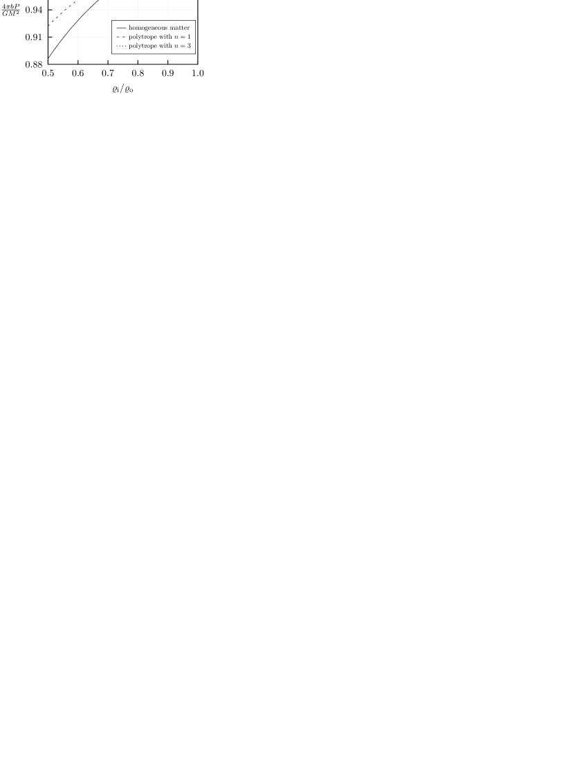
Figure 2: Numerical examples demonstrating how $4\pi bP/GM^{2}$ tends to 1 in the thin ring limit for various equations of state, cf. equation (23).

The terms from the expansion (10) of the potential in the vacuum that play a role up to first order are

$$A_{1} =2\int_{0}^{1}\mu_{00}y\,\text{d}y=\frac{M\sigma}{2\pi^{2}\mu_{\text{c}}a^{3}}$$ (24)

and

$$A_{2} =\frac{gM\sigma^{2}}{2\pi^{2}\mu_{\text{c}}a^{3}},\qquad g:=-\frac{\pi^{2}\mu_{\text{c}}a^{3}}{M\sigma}\int_{0}^{1}\mu_{00}y^{3}\,\text{d}y.$$ (25)

The coefficient $\Omega_{2}$ from the expansion of the square of the angular velocity is

$$\Omega_{2} =A_{1}(1+\lambda-2\beta_{11})+2A_{2}/\sigma$$ (26)

with

$$\lambda :=\ln(8/\sigma)-2,$$ (27)

and the constant of integration from the Euler equation is

$$\begin{split}V_{0}&=\left.\left(U_{\text{out}}-\frac{1}{2}\Omega^{2}\varrho^{2}\right)\right|_{r=r_{\text{s}}}\\ &=-\frac{GM}{2\pi b}\left(\frac{5\lambda+9}{2}+g-\beta_{11}\right).\end{split}$$ (28)

The term $g-\beta_{11}$ appearing in the above equation can be treated further by considering the rotational energy $T$ and potential energy $W$ and making use of the virial identity

$$\begin{split}0&=3P+2T+W\\ &=3P+\frac{GM^{2}}{\pi b}\left(g-\beta_{11}-\frac{1}{2}\right)\\ &\qquad-2\pi^{2}G\mu_{\text{c}}^{2}a^{4}b\int_{0}^{1}\mu_{00}h_{00}y\,\text{d}y.\end{split}$$ (29)

By restricting ourselves to the polytropic equation of state (see (34)), we can rewrite the above integral to read

$$\begin{split}\int_{0}^{1}\mu_{00}h_{00}y\,\text{d}y&=\frac{(n+1)K\mu_{\text{c}}^{1/n-1}}{Ga^{2}}\int_{0}^{1}\mu_{00}^{1+1/n}y\,\text{d}y\\ &=(n+1)\int_{0}^{1}p_{00}y\,\text{d}y=\frac{(n+1)M^{2}}{16\pi^{3}\mu_{\text{c}}^{2}a^{4}b^{2}},\end{split}$$ (30)

where the last step follows from (23). Putting this expression into (29) and using (23) again then yields

$$g-\beta_{11}=\frac{n-1}{8}.$$ (31)

Taking into account $1-\varrho_{\text{i}}/\varrho_{\text{o}}=2\sigma$, which holds to leading order, we can use (26) to write

$$\frac{2\pi b^{3}\Omega^{2}}{GM}+\ln\left(1-\frac{\varrho_{\text{i}}}{\varrho_{\text{o}}}\right)\to\frac{n-5}{4}+\ln 16$$ (32)

and (28) can be written as

$$\frac{4\pi bV_{0}}{5GM}-\ln\left(1-\frac{\varrho_{\text{i}}}{\varrho_{\text{o}}}\right)\to\frac{5-n}{20}-\ln 16$$ (33)

for polytropes in the thin ring limit. Similar equations can be derived for $J$ (angular momentum), $T$, $P$ and via the virial identity for $W$ (see Ostriker, 1964b). These equations also hold for homogeneous bodies ($n=0$), as was shown in Horatschek & Petroff (2008). Numerical examples demonstrating the behaviour (33) are provided in Fig. 3.

Figure 3: Numerical ring sequences (solid lines) for homogeneous matter (upper curve) and polytropes with $n=5$ (lower curve) are plotted for rings approaching the thin ring limit. The asymptotic behaviour as given by equation (33) is indicated by the dashed lines.

4 Mass Density for Polytropes at the Zeroth Order

The polytropic equation of state is

$$p=K\mu^{1+1/n}.$$ (34)

For large/small polytropic indices $n$, the equation is referred to as ‘soft’/‘stiff’ and as $n$ tends to zero, $\mu$ tends to a constant. From now on, we shall use the terms ‘homogeneous matter’ and ‘$n=0$’ interchangeably. For polytropes, (8) becomes

$$4\pi G\mu+K(n+1)\nabla^{2}\left(\mu^{1/n}\right)-2\Omega^{2}=0.$$ (35)

Instead of our coordinate $y$, we are now going to make use of a new dimensionless radial coordinate, applicable to polytropes

$$x:=\frac{G^{\frac{1}{2}}\mu_{\text{c}}^{\frac{n-1}{2n}}}{K^{\frac{1}{2}}}r.$$ (36)

To lowest order in $\sigma$, and upon introducing

$$\tilde{\mu}:=\mu^{1/n}$$ (37)

and the expansion

$$\tilde{\mu} =\mu_{\text{c}}^{1/n}\left(\sum_{i=0}^{q}\sum_{k=0}^{i}\tilde{\mu}_{ik}(x)\cos(k\chi)\sigma^{i}+o(\sigma^{q})\right),$$ (38)

equation (35) reads, cf. (15),

$$\left(\frac{\text{d}^{2}}{\text{d}x^{2}}+\frac{1}{x}\frac{\text{d}}{\text{d}x}\right)\tilde{\mu}_{00}+\frac{4\pi}{n+1}\tilde{\mu}_{00}^{n}=0.$$ (39)

This equation is sometimes referred to as one of the generalized Lane-Emden equations (of the first kind) and solutions to it have been derived and studied in e.g. Goenner & Havas (2000). No solutions other than for $n=1$ have been found for our particular parameters in closed-form and a discussion using symmetry transformations suggests that they do not exist, (Goenner, 2001). We thus concentrate in the next section on the special case $n=1$.

5 Analytic Solution for Polytropes with $\mn@boldsymbol{n=1}$

5.1 The Zeroth Order: $\mn@boldsymbol{\sigma^{0}}$

We rewrite (39) for $n=1$, remembering that now $\tilde{\mu}=\mu$,

$$\left(\frac{\text{d}^{2}}{\text{d}x^{2}}+\frac{1}{x}\frac{\text{d}}{\text{d}x}\right)\mu_{00}+2\pi\mu_{00}=0$$ (40)

and can immediately write down the general solution

$$\mu_{00}=C_{1}J_{0}(\sqrt{2\pi}x)+C_{2}Y_{0}(\sqrt{2\pi}x),$$ (41)

where $J_{n}$ is a Bessel function (of the first kind) and $Y_{n}$ a Neumann function (also called a Bessel function of the second kind), see e.g. Prudnikov, Brychkov & Marichev (1990). The condition $\mu(r=0,\chi)=\mu_{\text{c}}$ tells us that $C_{1}=1$ and $C_{2}=0$. The first positive zero of $J_{0}$ determines value for $a$ from (4). We refer to the $k$th positive zero of the $n$th Bessel function as $j_{nk}$ and can then write

$$ax/r=:\bar{a}=j_{01}/\sqrt{2\pi}=0.959\ldots$$ (42)

5.2 The First Order: $\mn@boldsymbol{\sigma^{1}}$

The unknown quantities we have to solve for are $\mu_{10}(x)$, $\mu_{11}(x)$, $\beta_{10}$, $\beta_{11}$, and $\Omega_{2}$. From (8), one finds the differential equations

$$\left(\frac{\text{d}^{2}}{\text{d}x^{2}}+\frac{1}{x}\frac{\text{d}}{\text{d}x}\right)\mu_{10}+2\pi\mu_{10}=0$$ (43)

and

$$\left(\frac{\text{d}^{2}}{\text{d}x^{2}}+\frac{1}{x}\frac{\text{d}}{\text{d}x}\right)\mu_{11}+\left(2\pi-\frac{1}{x^{2}}\right)\mu_{11}=\frac{1}{\bar{a}}\frac{\text{d}\mu_{00}}{\text{d}x}.$$ (44)

Considering only solutions that vanish at the point $x=0$, so as to maintain our choice $\mu(0)=\mu_{\text{c}}$, we find

$$\mu_{10} =0$$ (45)

and

$$\mu_{11} =C_{3}J_{1}+\frac{1}{2j_{01}}\left(\sqrt{2\pi}xJ_{0}-J_{1}\right),$$ (46)

where the argument of the Bessel function is always $\sqrt{2\pi}x$ unless otherwise specified. The requirement that the density vanish at the surface of the rings determines

$$\beta_{10}=0$$ (47)

and relates the constant $C_{3}$ to the surface function

$$C_{3}=\frac{1+2j_{01}^{2}\beta_{11}}{2j_{01}}.$$ (48)

The constant $\beta_{11}$ is determined by stipulating that the centre of mass coincide with the point $(\varrho=b,z=0)$ as in (9)

$$\beta_{11}=\frac{4-j_{01}^{2}}{4j_{01}^{2}}.$$ (49)

Recalling the definition $\lambda:=\ln\frac{8}{\sigma}-2$ one finally obtains

$$\Omega_{2}=\frac{2J_{1}(j_{01})(\lambda+1)}{j_{01}}$$ (50)

from (12).

5.3 The Second Order: $\mn@boldsymbol{\sigma^{2}}$

To second order, the unknown quantities that have to be solved for are $\mu_{20}(x)$, $\mu_{21}(x)$, $\mu_{22}(x)$, $\beta_{20}$, $\beta_{21}$, $\beta_{22}$, and $\Omega_{3}$.

The ODEs describing the mass density now read

$$\begin{split}&\left(\frac{\text{d}^{2}}{\text{d}x^{2}}+\frac{1}{x}\frac{\text{d}}{\text{d}x}\right)\mu_{20}+2\pi\mu_{20}=\pi\Omega_{2}\\ &\qquad+\frac{1}{2\bar{a}}\left(\frac{\text{d}\mu_{11}}{\text{d}x}-\frac{\mu_{11}}{x}\right)+\frac{x}{2\bar{a}^{2}}\frac{\text{d}\mu_{00}}{\text{d}x},\end{split}$$ (51)

$$\left(\frac{\text{d}^{2}}{\text{d}x^{2}}+\frac{1}{x}\frac{\text{d}}{\text{d}x}\right)\mu_{21}+\left(2\pi-\frac{1}{x^{2}}\right)\mu_{21}=\frac{1}{\bar{a}}\frac{\text{d}\mu_{10}}{\text{d}x}=0$$ (52)

and

$$\begin{split}&\left(\frac{\text{d}^{2}}{\text{d}x^{2}}+\frac{1}{x}\frac{\text{d}}{\text{d}x}\right)\mu_{22}+\left(2\pi-\frac{4}{x^{2}}\right)\mu_{22}=\\ &\qquad+\frac{1}{2\bar{a}}\left(\frac{\text{d}\mu_{11}}{\text{d}x}-\frac{\mu_{11}}{x}\right)+\frac{x}{2\bar{a}^{2}}\frac{\text{d}\mu_{00}}{\text{d}x}.\end{split}$$ (53)

The solutions vanishing at $x=0$ are

$$\mu_{20} =\frac{\Omega_{2}}{2}\left(1-J_{0}\right)+\frac{1}{8}\left[\frac{3\pi x^{2}}{j_{01}^{2}}J_{0}+\sqrt{2\pi}x\left(\frac{1}{j_{01}^{2}}-\frac{1}{2}\right)J_{1}\right],$$ (54)

$$\mu_{21} =C_{4}J_{1}$$ (55)

and

$$\begin{split}\mu_{22}&=C_{5}J_{2}+\frac{1}{4}\left[\left(\frac{5}{j_{01}^{2}}+\frac{3\pi x^{2}}{2j_{01}^{2}}-\frac{1}{2}\right)J_{2}\right.\\ &\qquad+\left.\frac{\sqrt{\pi}x}{\sqrt{2}}\left(\frac{5}{j_{01}^{2}}-\frac{1}{2}\right)J_{1}\right].\end{split}$$ (56)

The constants $C_{4}$ and $C_{5}$ can be related to the surface function by requiring that $\mu(r_{\text{s}})=0$ hold independently for the coefficients in front of $\cos\chi$ and $\cos 2\chi$. The result is

$$C_{4} =j_{01}\beta_{21}$$ (57)

and

$$C_{5} =\frac{1}{2}\left(-j_{01}^{2}\beta_{22}-\frac{j_{01}^{2}}{64}+\frac{3}{8}-\frac{11}{4j_{01}^{2}}\right).$$ (58)

Requiring the same of the coefficient in front of $\cos 0\chi$ gives

$$\beta_{20}=-\frac{4}{j_{01}^{4}}+\frac{\lambda+1}{j_{01}^{2}}-\frac{1}{64}.$$ (59)

Evaluating (9) tells us that

$$\beta_{21}=0\Longrightarrow\mu_{21}=0.$$ (60)

The values for the remaining constants follow from (12):

$$\Omega_{3}=0$$ (61)

and

$$\beta_{22}=\frac{1}{4j_{01}^{4}}+\frac{5(\lambda+3)}{2j_{01}^{2}}+\frac{1}{64}.$$ (62)

5.4 The Third Order: $\mn@boldsymbol{\sigma^{3}}$

The third order is the final one to be presented here, but the iterative scheme can be applied up to arbitrary order assuming that one is able to solve the differential equations for the mass density and perform the necessary integrals. The ODEs that result for this order are

$$\left(\frac{\text{d}^{2}}{\text{d}x^{2}}+\frac{1}{x}\frac{\text{d}}{\text{d}x}\right)\mu_{30}+2\pi\mu_{30}=0,$$ (63)

$$\begin{split}&\left(\frac{\text{d}^{2}}{\text{d}x^{2}}+\frac{1}{x}\frac{\text{d}}{\text{d}x}\right)\mu_{31}+\left(2\pi-\frac{1}{x^{2}}\right)\mu_{31}=\frac{3x^{2}}{4\bar{a}^{3}}\frac{\text{d}\mu_{00}}{\text{d}x}\\ &\quad+\frac{3}{4\bar{a}^{2}}\left(x\frac{\text{d}}{\text{d}x}+1\right)\mu_{11}+\frac{1}{\bar{a}}\left[\frac{\text{d}\mu_{20}}{\text{d}x}+\left(\frac{1}{2}\frac{\text{d}}{\text{d}x}+\frac{1}{x}\right)\mu_{22}\right],\end{split}$$ (64)

$$\left(\frac{\text{d}^{2}}{\text{d}x^{2}}+\frac{1}{x}\frac{\text{d}}{\text{d}x}\right)\mu_{32}+2\left(\pi-\frac{2}{x^{2}}\right)\mu_{32}=0$$ (65)

and

$$\begin{split}&\left(\frac{\text{d}^{2}}{\text{d}x^{2}}+\frac{1}{x}\frac{\text{d}}{\text{d}x}\right)\mu_{33}+\left(2\pi-\frac{9}{x^{2}}\right)\mu_{33}=\frac{x^{2}}{4\bar{a}^{3}}\frac{\text{d}\mu_{00}}{\text{d}x}\\ &\quad+\frac{1}{4\bar{a}^{2}}\left(x\frac{\text{d}}{\text{d}x}-1\right)\mu_{11}+\frac{1}{\bar{a}}\left(\frac{1}{2}\frac{\text{d}}{\text{d}x}-\frac{1}{x}\right)\mu_{22}.\end{split}$$ (66)

The solutions to these equations obeying the requirement $\mu_{qk}(0)=0$ are

$$\mu_{30} =0,$$ (67)

$$\begin{split}\mu_{31}&=\left(C_{6}-\frac{\left(\lambda+1\right)J_{1}\!\left(j_{01}\right)}{2j_{01}^{2}}-{\frac{9}{64}}{\frac{\pi\left(j_{01}^{2}-8\right){x}^{2}}{j_{01}^{3}}}\right.\\ &-\left.\frac{j_{01}^{4}+16j_{01}^{2}(5\lambda+4)-16}{256j_{01}^{3}}\right)J_{1}\\ &+\left(\frac{\sqrt{\pi}\left(\lambda+1\right)J_{1}\!\left(j_{01}\right)x}{\sqrt{2}j_{01}^{2}}-{\frac{15}{32}}{\frac{\sqrt{2}{\pi}^{3/2}{x}^{3}}{j_{01}^{3}}}\right.\\ &+\left.\frac{\sqrt{2\pi}\left(j_{01}^{4}+16j_{01}^{2}(5\lambda+4)-16\right)x}{256j_{01}^{3}}\right)J_{2},\end{split}$$ (68)

$$\mu_{32} =C_{7}J_{2}$$ (69)

and

$$\begin{split}\mu_{33}&=\frac{\pi{x}^{2}\left(16j_{01}^{2}(5\lambda+2)-40\pi{x}^{2}+272+j_{01}^{4}\right)}{512j_{01}^{3}}J_{1}\\ &\left(-\frac{5{\pi}^{2}{x}^{4}}{64j_{01}^{3}}+\frac{\pi\left(j_{01}^{4}+8j_{01}^{2}(10\lambda+7)+16\right)x^{2}}{512j_{01}^{3}}\right.\\ &-\left.\frac{3\left(j_{01}^{4}+16j_{01}^{2}(5\lambda+3)+208\right)}{256j_{01}^{3}}+C_{8}\right)J_{3}.\end{split}$$ (70)

The constants $\beta_{30}$, $C_{6}$, $C_{7}$ and $C_{8}$ are determined by requiring that $\mu(r=r_{\text{s}})=0$ hold independently for the coefficients in front of the $\cos 0\chi$, $\cos\chi$, $\cos 2\chi$ and $\cos 3\chi$ terms. The result is

$$\begin{split}\beta_{30}&=0,\\ C_{6}&=\left(\frac{\lambda+1}{4}-\frac{3\left(\lambda+1\right)}{2j_{01}^{2}}\right)J_{1}\!\left(j_{01}\right)-{\frac{j_{01}^{3}}{512}}\\ &\qquad+j_{01}\left(\frac{5}{32}\lambda+\beta_{31}+\frac{39}{256}\right)\\ &\qquad-\frac{14\lambda+9}{32j_{01}}+\frac{40\lambda+37}{16j_{01}^{3}},\end{split}$$ (71)

$$C_{7} =0$$ (72)

and

$$\begin{split}C_{8}&=\frac{1}{j_{01}^{2}-8}\Bigg{[}-{\frac{j_{01}^{5}}{1536}}-\left({\frac{5}{32}}\lambda+\beta_{33}+{\frac{77}{768}}\right)j_{01}^{3}\\ &\quad+\left({\frac{35}{16}}\lambda+{\frac{11}{8}}\right)j_{01}-\frac{1}{{j_{01}}}\left(10\lambda+{\frac{181}{48}}\right)-{\frac{119}{6j_{01}^{3}}}\Bigg{]}.\end{split}$$ (73)

Equation (9) yields

$$\beta_{31}={\frac{9}{32}}\lambda+{\frac{31}{128}}-\frac{1}{j_{01}^{2}}\left({\frac{13}{8}}\lambda+{\frac{5}{16}}\right)-\frac{1}{j_{01}^{4}}\left(\frac{5}{2}\lambda+9\right)$$ (74)

and (12) gives

$$\beta_{32} =0,$$ (75)

$$\begin{split}\Omega_{4}&=-2{\frac{\left(\lambda+1\right)^{2}}{j_{01}^{2}}}J_{1}\!\left(j_{01}\right)^{2}+\Bigg{[}\frac{1}{32}\left(\lambda+1\right)j_{01}\\ &\quad+{\frac{1}{j_{01}}}\left({\lambda}^{2}+\frac{3}{8}\lambda-\frac{1}{2}\right)\\ &\quad+\frac{1}{j_{01}^{3}}\left(\frac{11}{2}\lambda+{\frac{17}{4}}\right)\Bigg{]}J_{1}\!\left(j_{01}\right)\end{split}$$ (76)

and

$$\beta_{33} ={\frac{5}{64}}-\frac{1}{8j_{01}^{2}}\left(5\lambda+9\right)+\frac{1}{j_{01}^{4}}\left(\frac{5}{2}\lambda+2\right).$$ (77)

5.5 Physical Parameters

The shape of the rings to third order that results from equation (4) is compared to numerical results of the corresponding radius ratio in Fig. 4. For thin rings, the numerical and third order curves are indistinguishable. As the radius ratio is decreased, the numerical results show that the outer edge becomes pointier, right up to the mass-shedding limit for the value $\varrho_{\text{i}}/\varrho_{\text{o}}=0.25322\ldots$. For such a ring, a fluid particle rotating at the outer rim in the equatorial plane has a rotational frequency equal to the Kepler frequency, meaning that it is kept in balance by the gravitational and centrifugal forces alone – the force arising from the pressure gradient vanishes. The shape of the ring with the cusp that forms for mass-shedding configurations is not well represented by a small number of terms in our Fourier series.

Figure 4: Meridional cross-sections of polytropic rings ($n=1$) with varying radius ratio are shown to third order (solid lines) in comparison to numerical results (dashed lines) for the same radius ratio. At the value $\varrho_{\text{i}}/\varrho_{\text{o}}=0.25322\ldots$, the rings reach a mass-shedding limit, as is evident from the numerical cross-section.

Using the results of the last subsection, we write down expressions for various physical parameters and can use them to verify that the virial identity $3P+2T+W=0$ is satisfied to each order in $\sigma$. For convenience, we first introduce dimensionless quantities, valid for any polytropic index $n>0$:

$$\begin{split}\frac{\bar{M}}{M}=\frac{G^{\frac{3}{2}}\mu_{\text{c}}^{\frac{n-3}{2n}}}{K^{\frac{3}{2}}},\quad\frac{\bar{J}}{J}=\frac{G^{2}\mu_{\text{c}}^{\frac{2n-5}{2n}}}{K^{\frac{5}{2}}},\quad\frac{\bar{\Omega}}{\Omega}=\frac{1}{G^{\frac{1}{2}}\mu_{\text{c}}^{\frac{1}{2}}},\\ \frac{\bar{P}}{P}=\frac{\bar{T}}{T}=\frac{\bar{W}}{W}=\frac{G^{\frac{3}{2}}\mu_{\text{c}}^{\frac{n-5}{2n}}}{K^{\frac{5}{2}}},\quad\frac{\bar{b}}{b}=\frac{\bar{\varrho}}{\varrho}=\frac{G^{\frac{1}{2}}\mu_{\text{c}}^{\frac{n-1}{2n}}}{K^{\frac{1}{2}}},\end{split}$$ (78)

where $J$ refers to the angular momentum. Up to and including third order one finds

$$\begin{split}&\bar{M}=\,{\frac{\sqrt{2\pi}j_{01}^{2}J_{1}\!\left(j_{01}\right)}{\sigma}}\\ &\qquad+\bigg{[}\frac{\sqrt{2\pi}}{64}\left(j_{01}^{4}+28j_{01}^{2}+32j_{01}^{2}\lambda-16\right)J_{1}\!\left(j_{01}\right)\\ &\qquad-\sqrt{2\pi}j_{01}\left(\lambda+1\right)J_{1}\!\left(j_{01}\right)^{2}\bigg{]}\sigma,\end{split}$$ (79)

$$\begin{split}&\bar{J}=\,\sqrt{{\frac{J_{1}\!\left(j_{01}\right)\left(\lambda+1\right)}{j_{01}}}}J_{1}\!\left(j_{01}\right)j_{01}^{2}\Bigg{\{}\frac{j_{01}^{2}}{{\sigma}^{2}}\\ &\qquad-\frac{3}{2}\left(\lambda+1\right)j_{01}J_{1}\!\left(j_{01}\right)\\ &\qquad+{\frac{1}{128\left(\lambda+1\right)}}\big{[}3j_{01}^{4}(\lambda+1)\\ &\qquad+j_{01}^{2}(96{\lambda}^{2}+324\lambda+232)-624\lambda-664\big{]}\Bigg{\}},\end{split}$$ (80)

$$\begin{split}&\bar{P}=\,\frac{\sqrt{2\pi}}{2}j_{01}J_{1}\!\left(j_{01}\right)^{2}\bigg{\{}\frac{j_{01}^{2}}{\sigma}\\ &\qquad+\frac{1}{320}\Big{[}-640j_{01}\left(\lambda+1\right)J_{1}\!\left(j_{01}\right)\\ &\qquad+10\left(j_{01}^{4}-8j_{01}^{2}+128\lambda+136\right)\Big{]}\sigma\bigg{\}},\end{split}$$ (81)

$$\begin{split}&\bar{T}=\,\frac{\sqrt{2\pi}}{2}J_{1}\!\left(j_{01}\right)^{2}{j_{01}}\Bigg{\{}\frac{1}{\sigma}\left(\lambda+1\right)j_{01}^{2}\\ &\qquad\Big{[}-2\left(\lambda+1\right)^{2}J_{1}\!\left(j_{01}\right){j_{01}}+{\frac{1}{32}}\Big{(}j_{01}^{4}(\lambda+1)\\ &\qquad+2j_{01}^{2}(8\lambda+9)(2\lambda+3)-112\lambda-132\Big{)}\Big{]}\sigma\Bigg{\}}\end{split}$$ (82)

and

$$\begin{split}&\bar{W}=\,\sqrt{2\pi}j_{01}J_{1}\!\left(j_{01}\right)^{2}\Bigg{\{}-{\frac{j_{01}^{2}}{2\sigma}\left(2\lambda+5\right)}\\ &\qquad\Bigg{[}{j_{01}}\left(2\lambda+5\right)\left(\lambda+1\right)J_{1}\!\left(j_{01}\right)\\ &\qquad-{\frac{1}{64}}\Big{(}j_{01}^{4}(2\lambda+5)+4j_{01}^{2}(16{\lambda}^{2}+42\lambda+21)\\ &\qquad\qquad+160\lambda+144\Big{)}\Bigg{]}\sigma\Bigg{\}}.\end{split}$$ (83)

In the derivation of the above expressions for $\bar{P}$ and $\bar{W}$, we have made use of the identity

$$20\,_{2}\!F_{3}\!\left(\frac{3}{2},\frac{3}{2};2,2,\frac{5}{2};-j_{01}^{2}\right)=3j_{01}^{2}\,{}_{2}\!F_{3}\!\left(\frac{5}{2},\frac{5}{2};3,3,\frac{7}{2};-j_{01}^{2}\right)$$ (84)

for the Gauss hypergeometric function

$$\begin{split}&{}_{p}\!F_{q}(a_{1},a_{2},\ldots,a_{p};b_{1},b_{2},\ldots,b_{q};z)\\ &\qquad:=\sum_{k=0}^{\infty}\frac{{(a_{1})}_{k}\cdot{(a_{2})}_{k}\cdots{(a_{p})}_{k}}{{(b_{1})}_{k}\cdot{(b_{2})}_{k}\cdots{(b_{q})}_{k}}\frac{z^{k}}{k!}\end{split}$$ (85)

with the Pochhammer bracket

$${(a)}_{k}:=a(a+1)\cdots(a+k-1),\qquad{(a)}_{0}:=1.$$

A proof of (84) can be found in Appendix A.

In order to gauge the accuracy of the expressions listed above, some of them are plotted to first and third order in comparison to numerical values in Figs 5–7. The accuracy of the numerical values is high enough so as to render the corresponding curve indistinguishable from the ‘correct’ one and is plotted in its entirety, i.e. from the thin ring limit right up to the mass-shedding limit. The curves to first and third order were drawn by taking the expression for $\bar{\varrho}_{\text{i}}$, $\bar{\varrho}_{\text{o}}$, $\bar{\Omega}^{2}$, $\bar{M}$ and $\bar{J}$ to first and third order respectively, inserting a numerical value for $\sigma$ and then taking the appropriate combination of these numbers. One finds in all three plots that the third order brings a marked improvement as compared to the first one, but that the behaviour near the mass-shedding limit is not particularly well represented.

Figure 5: The square of the dimensionless angular velocity is plotted versus the radius ratio for rings with polytropic index $n=1$.

Figure 6: The dimensionless mass divided by the outer radius is plotted versus the radius ratio for rings with polytropic index $n=1$. This quantity tends to the value $\bar{M}/\bar{\varrho}_{\text{o}}=2\pi j_{01}J_{1}(j_{01})=7.84\ldots$ in the thin ring limit, which is marked by a tick.

Figure 7: The dimensionless angular momentum divided by the square of the outer radius is plotted versus the radius ratio for rings with polytropic index $n=1$. This quantity as a function of radius ratio tends logarithmically to infinity.

6 Solution for an Arbitrary Polytropic Index

As was mentioned above, our generalized Lane-Emden equation for $\tilde{\mu}_{00}$ can only be solved in closed-form for $n=1$. For other polytropic indices, the iterative method presented here was applied with the help of numerics. By describing the unknown density terms $\tilde{\mu}_{ik}$ by Chebyshev polynomials and expanding all the quantities involved in terms of $\lambda$, equations can be formulated for purely numerical coefficients. The equations of the approximation scheme described in Section 2 must be fulfilled, whereby the ODEs for $\tilde{\mu}_{ik}$ are evaluated at collocation points of the Chebyshev polynomials. In general, the density functions $\tilde{\mu}_{00}$ are not analytic at $x=\bar{a}$, meaning that high order polynomials may be necessary to find a good approximation of the function desired. We none the less chose this method, since the equations involve integrals over the density for which one end-point of integration contains the unknown surface function $r_{\text{s}}$, making their polynomial representation particularly useful.

If one is only interested in determining $\bar{a}$, $\beta_{11}$ and $\Omega_{2}$, then it is not necessary to combine such numerical and algebraic techniques and one can choose any numerical method for solving the ODEs. One begins by solving equation (39) numerically for the desired polytropic index $n$, prescribing the ‘initial conditions’ $\tilde{\mu}_{00}(0)=1$ and $\left.\frac{\text{d}}{\text{d}x}\tilde{\mu}_{00}\right|_{x=0}=0$. For spherical polytropic fluids, a surface of vanishing pressure is known to exist only for $n<5$, where the surface for $n=5$ extends out to infinity. The situation for polytropic rings is quite different – it seems that arbitrary polytropic indices are possible! Numerical solutions to (39) indicate that the density function $\mu_{00}$ indeed falls to zero for large $n$. The value of $x$ at the first zero of the solution is $\bar{a}$. One then proceeds to solve equation

$$\left(\frac{\text{d}^{2}}{\text{d}x^{2}}+\frac{1}{x}\frac{\text{d}}{\text{d}x}-\frac{1}{x^{2}}\right)\tilde{\mu}_{11}+\frac{4\pi n}{n+1}\tilde{\mu}_{00}^{n-1}\tilde{\mu}_{11}=\frac{1}{\bar{a}}\frac{\text{d}\tilde{\mu}_{00}}{\text{d}x}$$ (86)

for $\tilde{\mu}_{11}$ with the condition $\tilde{\mu}_{11}(0)=0$ and where $\left.\frac{\text{d}}{\text{d}x}\tilde{\mu}_{11}\right|_{x=0}$ has to be chosen so as to fulfil the centre of mass condition $\eqref{com}$ to first order, which reads

$$\begin{split}0&=\int_{0}^{\bar{a}}\mu_{11}x^{2}\,\text{d}x=n\int_{0}^{\bar{a}}\tilde{\mu}_{00}^{n-1}\tilde{\mu}_{11}x^{2}\,\text{d}x\\ \Longrightarrow 0&=\bar{a}^{2}\left.\frac{\text{d}\tilde{\mu}_{11}}{\text{d}x}\right|_{x=\bar{a}}-\bar{a}\tilde{\mu}_{11}(\bar{a})+\frac{2}{\bar{a}}\int_{0}^{\bar{a}}\tilde{\mu}_{00}x\,\text{d}x.\end{split}$$ (87)

The constant $\beta_{11}$ can then be found using equation (19), which now reads

$$\beta_{11} =-\frac{\tilde{\mu}_{11}(\bar{a})}{\bar{a}}\left.\left(\frac{\text{d}\tilde{\mu}_{00}}{\text{d}x}\right)^{-1}\right|_{x=\bar{a}},$$ (88)

and $\Omega_{2}$ is taken from (32). The behaviour of these coefficients as they depend on the polytropic index $n$ can be found in Table 1. The table suggests that $\bar{a}\to\infty$ and $\Omega_{2}\to 0$ exponentially in $n$ for $n\to\infty$, which is indeed known to hold (Ostriker, 1964a, b). The behaviour of the specific kinetic energy of a particle in the ring, proportional to $\bar{a}^{2}\Omega_{2}$ to leading order, will be discussed in the next subsection together with the behaviour of $\beta_{11}$ for large $n$.

Table 1: The values of expansion coefficients for the surface function $r_{\text{s}}$ and for the squared angular velocity are provided up to first order for different polytropic indices $n$. The value of $\bar{a}$ for $n=0$ can be found by solving (39) with $n=0$ and the conditions $\frac{\text{d}}{\text{d}x}\tilde{\mu}_{00}|_{x=0}=0$ and $\tilde{\mu}_{00}(0)=1$ and then locating the first zero of $\tilde{\mu}_{00}$.

$n$	$\bar{a}$	$\beta_{11}$	$\Omega_{2}$
0	$1/\sqrt{\pi}\approx 0.5642$	0	$\lambda+3/4$
0.5	$0.7566$	$-0.03537$	$0.6371\lambda+0.5575$
1	$0.9594$	$-0.07708$	$0.4318(\lambda+1)$
2	$1.427$	$-0.1731$	$0.2169\lambda+0.2711$
5	$3.750$	$-0.5118$	$0.03614\lambda+0.07228$
10	$15.18$	$-1.126$	$(2.401\lambda+7.804)\times 10^{-3}$
20	$207.6$	$-2.375$	$(1.362\lambda+7.829)\times 10^{-5}$
30	$2.661\times 10^{3}$	$-3.625$	$(8.487\lambda+70.02)\times 10^{-8}$
40	$3.337\times 10^{4}$	$-4.875$	$(5.468\lambda+58.78)\times 10^{-10}$
50	$4.142\times 10^{5}$	$-6.125$	$(3.577\lambda+47.40)\times 10^{-12}$

Before doing so, we provide a comparison of precise numerical values for various physical quantities with their first order equivalents in Table 2. One can see that the accuracy of the method does not depend strongly on the polytropic index and that relative errors are within a few percent for rings with a radius ratio of 0.9.

Table 2: Physical quantities to the first order in $\sigma$ (bold faced type) are compared to the correct, numerically determined values (normal type) for given polytropic index $n$ and given radius ratio $\varrho_{\text{i}}/\varrho_{\text{o}}=0.9$.

$n$	$\bar{M}$	$\bar{\Omega}^{2}$	$\bar{J}$	$\bar{P}$	$\bar{T}$	$\bar{W}$
0.5	103	0.0216	$\mathbf{3.14\times 10^{3}}$	59.2	231	$\mathbf{-640}$
0.5	105	0.0213	$3.21\times 10^{3}$	59.9	235	$-650$
1	143	0.0151	$\mathbf{5.84\times 10^{3}}$	89.2	359	$\mathbf{-986}$
1	144	0.0150	$5.95\times 10^{3}$	90.1	364	$-999$
3	356	$\mathbf{4.56\times 10^{-3}}$	$\mathbf{3.53\times 10^{4}}$	264	$\mathbf{1.19\times 10^{3}}$	$\mathbf{-3.17\times 10^{3}}$
3	359	$4.52\times 10^{-3}$	$3.58\times 10^{4}$	266	$1.20\times 10^{3}$	$\mathbf{-3.21\times 10^{3}}$
5	714	$\mathbf{1.58\times 10^{-3}}$	$\mathbf{1.44\times 10^{3}}$	570	$\mathbf{2.86\times 10^{3}}$	$\mathbf{-7.44\times 10^{3}}$
5	720	$1.56\times 10^{-3}$	$1.46\times 10^{3}$	575	$2.89\times 10^{3}$	$-7.51\times 10^{3}$

7 The Limit of Infinite Polytropic Index

As $n$ tends to infinity, the polytropic equation (34) shows us that pressure and density are proportional

$$p=K\mu,$$ (89)

a case sometimes referred to as ‘isothermal’ because such an equation holds for an ideal gas at constant temperature. Inserting this into equation (35) at leading order and again using the dimensionless coordinate $x$ yields

$$4\pi x\mu_{00}+\frac{\text{d}}{\text{d}x}\left(x\frac{\text{d}}{\text{d}x}\ln\mu_{00}\right)=0.$$ (90)

The solution to this equation with our normalization $\mu_{00}(x=0)=1$ reads

$$\mu_{00}=\frac{4}{\pi^{2}\left(x^{2}+\frac{2}{\pi}\right)^{2}}.$$ (91)

The density and pressure fall to zero as $x\to\infty\Leftrightarrow r\to\infty$. Integrating over the density to calculate the normalized mass, one finds to leading order

$$\bar{M}=4\pi^{2}\bar{b}\int_{0}^{\infty}\mu_{00}x\,\text{d}x=4\pi\bar{b},$$ (92)

which can also be read off from equation (23) directly, by making use of $\bar{M}=\bar{P}$, which is self-evident upon taking (89) into account. In Fig. 8, the behaviour of $\bar{M}/4\pi\bar{b}$ can be followed from the homogeneous case, $n=0$, right up to the isothermal limit $n\to\infty$.

Figure 8: The dimensionless mass divided by $4\pi\bar{b}$ in the thin ring limit is plotted versus $n/(n+1)$ over the whole range of polytropic indices $n\in[0,\infty)$. The points for $n=0$, $n=1$ and $n\to\infty$ are known analytically and the remainder of the curve was generated by solving the equation for $\tilde{\mu}_{00}$ numerically and making use of equation (20).

Making use of (91), we find that

$$\lim_{n\to\infty}g=0,$$ (93)

where $g$ was defined in (25). It thus follows from (31) that

$$\lim_{n\to\infty}\left(\beta_{11}+\frac{n}{8}\right)=\frac{1}{8}$$ (94)

as already suggested by the results of Table 1. We can then see that the specific kinetic energy $\bar{a}^{2}\Omega_{2}$ tends to infinity such that for fixed $\lambda$

$$\lim_{n\to\infty}\frac{2\pi\bar{a}^{2}\Omega_{2}}{n+4\lambda}=1.$$ (95)

From the fact that $|\beta_{11}|$ tends to infinity, we can conclude that the range of $\sigma$ values for which the first order provides a good approximation shrinks to the point $\sigma=0$. This provides us with evidence suggesting that the deviation in a ring’s cross-section from a circle becomes more pronounced at a given radius ratio as $n$ is increased. The value for $\varrho_{\text{i}}/\varrho_{\text{o}}$ at which one reaches the mass-shedding limit presumably tends to 1 as $n$ tends to infinity.

Appendix A An Identity Relating Hypergeometric to Bessel Functions

In order to prove the identity (84), we prove the more general identity

$$\begin{split}&\frac{3}{40}z\,_{2}\!F_{3}\left(\frac{5}{2},\frac{5}{2};3,3,\frac{7}{2};-z\right)-\frac{1}{2}\,_{2}\!F_{3}\left(\frac{3}{2},\frac{3}{2};2,2,\frac{5}{2};-z\right)\\ &\qquad=\frac{\text{d}}{\text{d}z}\left[J_{0}(\sqrt{z})^{2}\right],\end{split}$$ (96)

for an arbitrary complex number $z$, from which (84) follows immediately.

We begin by using the differentiation properties of the hypergeometric functions, e.g. 7.2.3.47 in Prudnikov et al. (1990), to write

$$\begin{split}&\frac{3}{40}\,\,_{2}\!F_{3}\left(\frac{5}{2},\frac{5}{2};3,3,\frac{7}{2};-z\right)z-\frac{1}{2}\,\,_{2}\!F_{3}\left(\frac{3}{2},\frac{3}{2};2,2,\frac{5}{2};-z\right)\\ &\qquad=\frac{\text{d}}{\text{d}z}\Bigg{[}\,_{2}\!F_{3}\left(\frac{1}{2},\frac{1}{2};1,1,\frac{3}{2};-z\right)\\ &\qquad\qquad\qquad-\frac{z}{3}\,\,_{2}\!F_{3}\left(\frac{3}{2},\frac{3}{2};2,2,\frac{5}{2};-z\right)\Bigg{]}.\end{split}$$ (97)

With the integral identity 7.2.3.11, the term to be differentiated can be written as

$$\begin{split}&{}_{2}\!F_{3}\left(\frac{1}{2},\frac{1}{2};1,1,\frac{3}{2};-z\right)-\frac{z}{3}\,\,_{2}\!F_{3}\left(\frac{3}{2},\frac{3}{2};2,2,\frac{5}{2};-z\right)\\ &\quad=\frac{1}{\pi}\int_{0}^{1}\!\!\!\int_{0}^{1}\frac{J_{0}(2\sqrt{t_{1}t_{2}z})}{2\sqrt{t_{1}t_{2}(1-t_{1})}}-\frac{zJ_{1}(2\sqrt{t_{1}t_{2}z})}{2\sqrt{z(1-t_{1})}}\,\text{d}t_{1}\,\text{d}t_{2},\end{split}$$ (98)

where we have made use of the identity (e.g. 7.13.1.1 in Prudnikov et al. 1990)

$${}_{0}\!F_{1}(b,-z)=\Gamma(b)z^{(1-b)/2}J_{b-1}(2\sqrt{z}).$$ (99)

The above double integral yields

$$\begin{split}&\frac{1}{\pi}\int_{0}^{1}\!\!\!\int_{0}^{1}\frac{J_{0}(2\sqrt{t_{1}t_{2}z})}{2\sqrt{t_{1}t_{2}(1-t_{1})}}-\frac{zJ_{1}(2\sqrt{t_{1}t_{2}z})}{2\sqrt{z(1-t_{1})}}\,\text{d}t_{1}\,\text{d}t_{2}\\ &\qquad=\frac{1}{\pi}\int_{0}^{1}\frac{J_{0}(2\sqrt{t_{1}z})}{t_{1}(1-t_{1})}\text{d}t_{1}=J_{0}(\sqrt{z})^{2},\end{split}$$ (100)

thereby proving (96).

References

• Ansorg etΒ al. (2003a) Ansorg M., KleinwΓ€chter A., Meinel R., 2003a, Astron.Β Astrophys., 405, 711
• Ansorg etΒ al. (2003b) Ansorg M., KleinwΓ€chter A., Meinel R., 2003b, Astrophys.Β J.Β Lett., 582, L87
• Ansorg etΒ al. (2003c) Ansorg M., KleinwΓ€chter A., Meinel R., 2003c, Mon.Β Not.Β R.Β Astron.Β Soc., 339, 515
• Ansorg & Petroff (2005) Ansorg M., Petroff D., 2005, Phys.Β Rev.Β D, 72, 024019
• Chandrasekhar & Fermi (1953) Chandrasekhar S., Fermi E., 1953, ApJ, 118, 116
• Dyson (1892) Dyson F.Β W., 1892, Philos.Β Trans.Β R.Β Soc.Β London, Ser. A, 184, 43
• Dyson (1893) Dyson F.Β W., 1893, Philos.Β Trans.Β R.Β Soc.Β London, Ser. A, 184, 1041
• Eriguchi & Hachisu (1985) Eriguchi Y., Hachisu I., 1985, Astron.Β Astrophys., 148, 289
• Eriguchi & Sugimoto (1981) Eriguchi Y., Sugimoto D., 1981, Prog.Β Theor.Β Phys., 65, 1870
• Fischer etΒ al. (2005) Fischer T., Horatschek S., Ansorg M., 2005, Mon.Β Not.Β R.Β Astron.Β Soc., 364, 943
• Goenner (2001) Goenner H., 2001, Gen.Β Rel.Β Grav., 33, 833
• Goenner & Havas (2000) Goenner H., Havas P., 2000, J.Β Math.Β Phys., 41, 7029
• Hachisu (1986) Hachisu I., 1986, ApJS, 61, 479
• Horatschek & Petroff (2008) Horatschek S., Petroff D., 2008, arXiv:0802.0078
• Kowalewsky (1885) Kowalewsky S., 1885, Astronomische Nachrichten, 111, 37
• Lichtenstein (1933) Lichtenstein L., 1933, Gleichgewichtsfiguren rotierender FlΓΌssigkeiten. Springer, Berlin
• Ostriker (1964a) Ostriker J., 1964a, ApJ, 140, 1056
• Ostriker (1964b) Ostriker J., 1964b, ApJ, 140, 1067
• Ostriker (1965) Ostriker J., 1965, ApJ, 11, 167
• PoincarΓ© (1885) PoincarΓ© H., 1885, Acta mathematica, 7, 259
• Prudnikov etΒ al. (1990) Prudnikov A.Β P., Brychkov Y.Β A., Marichev O.Β I., 1990, Integrals and Series. Vol.Β 3, Gordon and Breach Science Publishers, New York
• Wong (1974) Wong C.Β Y., 1974, Astrophys.Β J., 190, 675