Spectral Identification of an Ancient Supernova using Light Echoes in the LMC

Abstract

We report the successful identification of the type of the supernova responsible for the supernova remnant SNR 0509-675 in the Large Magellanic Cloud (LMC) using Gemini spectra of surrounding light echoes. The ability to classify outbursts associated with centuries-old remnants provides a new window into several aspects of supernova research and is likely to be successful in providing new constraints on additional LMC supernovae as well as their historical counterparts in the Milky Way Galaxy (MWG). The combined spectrum of echo light from SNR 0509-675 shows broad emission and absorption lines consistent with a supernova (SN) spectrum. We create a spectral library consisting of 26 SNe Ia and 6 SN Ib/c that are time-integrated, dust-scattered by LMC dust, and reddened by the LMC and MWG. We fit these SN templates to the observed light echo spectrum using $\chi^{2}$ minimization as well as correlation techniques, and we find that overluminous 91T-like SNe Ia with ${\Delta m_{15}}<0.9$ match the observed spectrum best.

1. Introduction

Over 100 years ago, a rapidly expanding nebula was photographed by Ritchey around Nova Persei 1901 (Ritchey, 1901a, b, 1902), and it was interpreted as a light echo from the nova explosion (Kapteyn, 1902). Later modelling of the physics of the scattering and the geometry that lead to apparent superluminal expansion confirmed this interpretation (Couderc, 1939). Since then, light echoes (whereby we mean a simple scattering echo rather than fluorescence or dust re-radiation) have been seen in the Galactic Nova Sagittarii 1936 (Swope, 1940) and the eruptive variable V838 Monocerotis (Bond et al., 2003). Echoes have also been observed from extragalactic supernovae, with SN 1987A being the most famous case (Crotts, 1988; Suntzeff et al., 1988; Newman & Rest, 2006), but also including SNe 1991T (Schmidt et al., 1994; Sparks et al., 1999), 1993J (Sugerman & Crotts, 2002; Liu et al., 2003), 1995E (Quinn et al., 2006), 1998bu (Cappellaro et al., 2001), 2002hh (Welch, 2007), and 2003gd (Sugerman, 2005; Van Dyk et al., 2006).

By simple scaling arguments based on the visibility of Nova Persei (Shklovskii, 1964; van den Bergh, 1965, 1975), light echoes from supernovae as old as a few hundred to a thousand years can be detected, especially if the illuminated dust has regions of high density ($\geq 10^{-8}\rm{cm}^{-3}$). More sophisticated models of scattered light echoes have been published (Chevalier, 1986; Sugerman, 2003; Patat, 2005) but the tabulations do not predict late-time light echo surface brightness.

The few targeted surveys for light echoes from supernovae (van den Bergh, 1966; Boffi et al., 1999) and novae (van den Bergh, 1977; Schaefer, 1988) have been unsuccessful. However, these surveys did not use digital image subtraction techniques to remove the dense stellar and galactic backgrounds. Even the bright echoes near SN 1987A (Suntzeff et al., 1988) at $V\approx 21.3\ \rm{mag\ arcsec}^{-2}$ are hard to detect relative to the dense stellar background of the Large Magellanic Cloud (LMC).

During the five observing seasons allocated to SuperMACHO Project observations, the LMC was observed repeatedly using the Mosaic imager at the Cerro Tololo Interamerican Observatory (CTIO) Blanco 4m telescope. An automated image reduction pipeline performed high-precision difference-imaging from September 2001 to December 2005. We discovered light echo systems associated with three ancient SNe in the LMC. The echo motions trace back to three of the youngest supernova remnants (SNRs) in the LMC: SNR 0519-69.0, SNR 0509-67.5, and SNR 0509-68.7 (N103B). These three remnants have also been identified as Type Ia events, based on the X-ray spectral abundances (Hughes et al., 1995). We have dated these echoes to events 400-800 years ago using their position and apparent motion (Rest et al., 2005b). Such light echo systems provide the extraordinary opportunity to study the spectrum of the light from SN explosions that reached Earth hundreds of years ago, determine their spectral types, and compare them to now well-developed remnant structures and elemental residues.

We have obtained spectra of light echoes from each of the three light echo groups with the Gemini-South GMOS spectrograph. While the light echoes of SNR 0519-69.0 and 0509-68.7 are in very crowded regions of the LMC bar, the light echo features associated with SNR 0509-67.5 are in a much less confused area. They are also the brightest light echo features we have discovered to date. We have extracted the light echo spectrum associated with SNR 0509-67.5 applying standard reduction techniques.

The stellar spectral LMC background cannot be completely removed from the fainter light echo features of SNR 0519-69.0 and 0509-68.7. We have obtained multi-object spectra with using GMOS on Gemini South separated in time by one year in order to subtract off the stationary stellar spectral background and retain the (apparently moving) supernova echo light. In this paper we discuss the analysis of the light echo spectrum of SNR 0509-67.5, and we determine the SN spectral type. We defer the analysis of the light echo spectrum of SNR 0519-69.0 and 0509-68.7 to a future paper.

2. Observations & Reductions

2.1. Data Reduction of Imaging Observations

The SuperMACHO Project microlensing survey monitored the central portion of the LMC with a cadence of every other night during the five fall observing seasons beginning with September 2001. The CTIO 4m Blanco telescope with its 8Kx8K MOSAIC imager and atmospheric dispersion corrector were used to cover a mosaic of 68 pointings in an approximate rectangle $3.7\deg$ by $6.6\deg$ aligned with the LMC bar. The images are taken through our custom “VR” filter ($\lambda_{c}=625\ \rm{nm}$, $\delta\lambda=220\ \rm{nm}$, NOAO Code c6027) with exposure times of 60 s to 200 s, depending on the stellar densities. We used an automated pipeline to subtract PSF-matched template images from the most recently acquired image to search for variability (Rest et al., 2005a; Garg et al., 2007; Miknaitis et al., 2007). The resulting difference images are remarkably clean of the (constant) stellar background and are ideal for searching for variable objects. Our pipeline detects and catalogs the variable sources.

While searching for microlensing events in the LMC, we detected groups of light echoes pointing back to three SNRs in the LMC, SNR 0519-69.0, SNR 0509-67.5, and SNR 0509-68.7 (N103B). The surface brightnesses of the light echoes ranged from $22.5\ \rm{mag\ arcsec}^{-2}$ to the detection limit of the survey of about $24\ \rm{mag\ arcsec}^{-2}$.

2.2. Spectroscopic Observations

Images were obtained on UT 2005 September 7 in the $r^{\prime}$ band using the Gemini-S GMOS spectrograph covering a 5.5 $\times$ 5.5 arcmin field centered on the brightest echoes associated with SNR 0509-675. These pre-images were used to design a focal plane mask which included slitlets on 9 echoes, 9 stars, and 28 blank sky regions. The slits were 1.0 arcsec wide. Spectroscopy was obtained using GMOS with the R400 grating, yielding a resolution of 0.8Å and a spectral range of 4500-8500Å.

Spectroscopic observations were obtained on UT 2005 Nov 7, 2005 Dec 6 and 2005 Dec 7. A total of six hour-long observations were made. The data were taken using the nod-and-shuffle technique (Glazebrook & Bland-Hawthorn, 2001), with the telescope nodded between the on source position and a blank sky field located 4 degrees away (off the LMC) every 120 seconds. In total, 3 hours were spent integrating on-source. CuAr spectral calibration images and GCAL flatfields were interspersed with the science observations. The nod-and-shuffle technique provides for the best possible sky subtraction despite strong fringing in the red for the CCDs.

2.3. Data Reduction of Spectroscopic Observations

The GMOS data were processed using IRAF and the Gemini IRAF package. The GMOS data was written as multi-extension FITS files with three data extensions, one for each of the three CCDs in the instrument. We performed the initial processing by extension (that is, by CCD), waiting until after nod and shuffle subtraction to mosaic the extensions into a single array. First, an overscan value was subtracted and unused portions of the array were trimmed. As the CCD was dithered after each nod and shuffle observation in order to reduce the effects of charge traps, a separate flat field was obtained for each science observation. The flat field images were fit with a low-order spline for normalization and then each science frame was flattened with the appropriate normalized flat. Both “A” and “B” nods in a given frame were flattened with the same flat. The Gemini IRAF package gnscombine was used to combine all the observations of a given light echo while also performing the subtraction of the nod and shuffle components. The individual extensions were then mosaicked into a single array.

Since the slitlets were oriented at various position angles tangent to the bright portions of the echo, each individual slitlet had to be rectified using a geometric transformation derived from the CuAr calibration lamp spectra. The slitlets with the brightest echo features were extracted by collapsing each slitlet along the spatial dimension. Wavelength calibration provided by the CuAr calibration lamps were taken through the same mask. A low-order polynomial was fit to the calibration lamp spectra and the solution then applied to each slitlet. The three brightest individual slitlets could then be combined. A slitlet that had been purposely placed in an apparently blank portion of the field was then used to create a background spectrum to represent the diffuse spectral background of the LMC. This background was scaled and subtracted from the one-dimensional combined spectrum of the echo. Despite these efforts, some residual spectral contamination remains, as evidenced by narrow emission lines in the final spectrum.

We used the spectrophotometric standard LTT 4364 (Hamuy et al., 1992, 1994) to flux-calibrate the individual spectra using our own routines in IDL. The standard star was not observed on the same nights as the echo observations. The relative spectrophotometry is expected to be good at the 5% level based on our extensive experience with the reduction of a large sample of low-z Type Ia SNe for which we have photometry and spectroscopy(Matheson, 2007). We also used LTT 4364 to remove telluric features from the spectra using techniques described by Wade & Horne (1988); Bessell (1999); Matheson et al. (2000). Figure 1 shows the reduced spectrum of the light echo associated with SNR 0509-675, which exhibits broad emission and absorption features consistent with SN spectra.

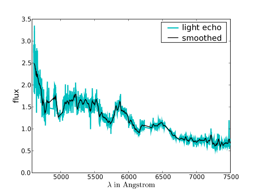
Figure 1.— Observed spectrum of a light echo assicated with SNR 0509-675 (cyan line). We have removed the chip gaps (4838Å-4894Å, 6235Å-6315Å), and various LMC background emission lines ([O III], H$\alpha$, [N II], [S II]). The black line indicates the boxcar-smoothed spectrum. The broad absorption and emission lines are consistent with SN spectra.

3. Analysis

Several authors have addressed the scattering of light off dust particles and its effect on the surface brightness and spectrum of the resulting light echoes (Couderc, 1939; Chevalier, 1986; Emmering & Chevalier, 1989; Sugerman, 2003; Patat, 2005; Patat et al., 2006, e.g.). The light echo spectrum can be described by the time-integrated SN spectrum attenuated by the scattering dust (Sugerman, 2003; Patat et al., 2006). First, we describe how we create our library of 26 time-integrated SN Ia spectra and 6 time-integrated SN Ib/c spectra (see Section 3.1). Since our goal is to compare SN spectra, we introduce and describe methods to correlate and compare SN spectra in Section 3.2, and we test these methods by comparing the integrated SN Ia template spectra. We introduce a technique that estimates the $\Delta m_{15}$ of a given SN Ia based on its correlation with other SNe Ia. In Section 3.3 we describe how the spectrum is attenuated by the scattering dust. We then test in Section 3.4 our method to estimate the $\Delta m_{15}$ of a SNe by correlating its light echo with dust-scattered, time-integrated SNe Ia template on the example of SN 1998bu.

3.1. Time-integrated Spectra

The observed light echo is derived from scattering of the supernova light off of dust sheets. These dust sheets have light time travel dimensions which are significant with respect to the duration of a supernova’s pre-nebular phase. Thus, the light echo represents a time-integration of the supernova flux attenuated by the scattering dust (Sugerman, 2003; Patat et al., 2006). We create 26 time-integrated SN Ia spectra using the lightcurve and spectral library of Matheson (2007); Jha et al. (2006), and 6 time-integrated SN Ib/c using the data references shown in Column (10) in Table 2. We cannot use a simple integration algorithm, like the trapezoidal rule, since there are often significant gaps of sometimes up to 15 days in coverage due to bright time, weather conditions, and schedule constraints. Simple interpolation over non-homogenous coverage would not correctly account for the non-linear shape of the SNe lightcurves. Thus we calculate for each day a spectrum as the weighted average of its two closest in time input spectra and scale it so that the spectrum convolved with the $V$ filter agrees with the magnitude from the lightcurve fit. Then we use the trapez rule to integrate. All these steps are simple weighted summations of the input spectra, and can be combined to a weighted sum of all the input spectrum. Since we have normalized the input spectrum so that the spectra convolved with the $V$ filter have the same reference magnitude $V=15$, these weights have the added benefit that they indicate the contribution of each input spectrum to the final integrated spectrum. This gives us the means to test if one or two input spectra dominate the integrated spectrum due to imperfect coverage: If the maximum weight is large, it is an indication of such problems. We use this maximum weight as a tool to grade the integrated spectra. In detail, we perform the following steps on each SN:

• The spectral templates $\hat{S}_{i}$ at epochs $\hat{t}_{i}$ are normalized so that the spectra convolved with the $V$ filter have the same reference magnitude $V=15$.

• We fit $V$-band lightcurve templates of SN Ia (Prieto et al., 2006) and SN Ib/c (P. Nugent online library) to the observed lightcurves. These fitted lightcurves range from -15 days to +85 days with respect to the B-band maximum.

• For a given time $t_{k}$, we find the spectra that are closest to this date in both time directions, $\hat{t}^{-}_{i1}$ and $\hat{t}^{+}_{i2}$. We estimate the spectrum as the time-weighted average of these two spectra with $c_{i1}(t_{k})=(\hat{t}^{-}_{i2}-t_{k})/(\hat{t}^{+}_{i2}-\hat{t}^{-}_{i1})$ and $c_{i2}(t_{k})=(t_{k}-\hat{t}^{-}_{i1})/(\hat{t}^{+}_{i2}-\hat{t}^{-}_{i1})$. For times before the first or after the last spectrum, we just use the first and last spectrum, respectively. Then we normalize the spectrum by $n(t_{k})$ so that the spectrum convolved with the $V$ filter agrees with the magnitude from the lightcurve fit.

  $$S(t_{k})=n(t_{k})*(c_{i1}(t_{k})\hat{S}_{i1}+c_{i2}(t_{k})\hat{S}_{i2})$$ (1)

• We integrate the spectrum from -15 days to +85 days with respect to the $B$ band maximum. Calculating the integrated spectrum is thus just a linear combination of the input template spectra $\hat{S}_{i}$

  $$F(\lambda) = \sum_{k}S(t_{k})$$ (2)

  $$= \sum_{j}w_{j}\hat{S}_{j}$$ (3)

  where the $w_{j}$ are functions of $n(t_{k})$ and $c_{i}(t_{k})$.

As outlined before, the dominant complication creating the time-integrated spectra is that for a given SN, the epochs for which spectra are available are non-homogenous, and one or two spectra can end up dominating the integrated spectrum. If the maximum weight $w_{max}=maximum(w_{j})$ is large, it is an indication of such problems. To reflect the relative quality of this effect, we grade our integrated spectra by requiring that for grade $A$, $B$, and $C$ the maximum weight fulfills $w_{max}\leq 25$%, $w_{max}\leq 35$%, and $w_{max}\leq 45$%, respectively. We find 13, 7, and 8 SNe Ia of grade $A$, $B$, and $C$, respectively (see Table 1). For the SNe of type Ib/c, we find 3, 2, and 1 of grade $A$, $B$, and $C$, respectively (see Table 2).

3.2. Methods to Compare and Correlate Spectra

Our ultimate goal is to find the time-integrated template spectra that match best the observed light echo spectrum in order to determine the (sub)type of the SNe. One possibility is to fit the template spectra to the observed light echo spectrum by a simple normalization and calculate the $\chi^{2}$. The intrinsic problem with a $\chi^{2}$-minimization fit of spectra is that already small but low spatial frequency errors such as those due to errors in dereddening or background subtraction can warp the spectrum and lead to a bad measure of fit. An alternative to the $\chi^{2}$-minimization approach is the cross-correlation technique. In this paper, we use an implementation of the correlation techniques of Tonry & Davis (1979), the SuperNova IDentification code (SNID; Blondin & Tonry 2006, 2007). We compare and correlate the template SN Ia spectra: Do the templates correlate better if they have similar ${\Delta m_{15}}$? Can we determine the ${\Delta m_{15}}$ of a SNe template just by correlating it to the other SNe Ia templates? In the following we discuss the advantages and disadvantages of these techniques.

3.2.1 $\chi^{2}$-minimization

We compare each SN Ia template spectrum with all others by performing a $\chi^{2}$-minimization fit with a normalization factor as the only free parameter. We use the variance spectrum as $1-\sigma$ errors for the observed spectrum. Figure 2 shows the $\chi^{2}$ versus their difference in ${\Delta m_{15}}$: $\Delta m_{15}(i)-\Delta m_{15}(j)$ for all SN Ia with grade $A$ or $B$. There is a trend that for smaller differences in ${\Delta m_{15}}$ the $\chi^{2}$ is smaller, indicating that indeed SN Ia with similar ${\Delta m_{15}}$ have similar spectra. However, there is still a big spread. This is most likely due to errors in dereddening or galaxy subtraction introducing systematic errors. Figure3 shows the spectra of SN 1999dq and SN 1999aa. The spectrum of SN 1999aa is very similar to the spectrum of SN 1999dq, with the exception that the SN 1999aa spectrum is warped toward the blue. This difference is most likely not real but an artifact of dereddening or background subtraction.

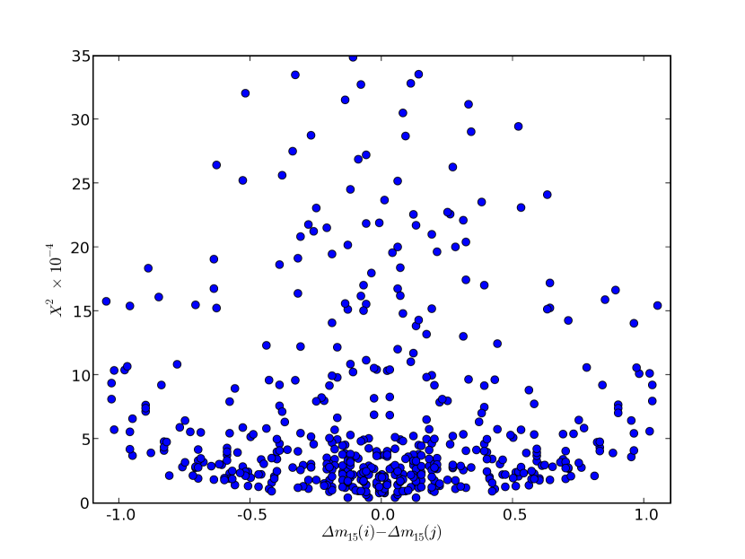
Figure 2.— This figure shows the $\chi^{2}$ versus their difference in ${\Delta m_{15}}$: $\Delta m_{15}(i)-\Delta m_{15}(j)$ for all SN Ia in category $A$ and $B$. There is a trend that for smaller differences in ${\Delta m_{15}}$ the $\chi^{2}$ is smaller, indicating that indeed SN Ia with similar ${\Delta m_{15}}$ are more similar. However, there is still a large spread which is most likely due to errors in dereddening or galaxy subtraction.

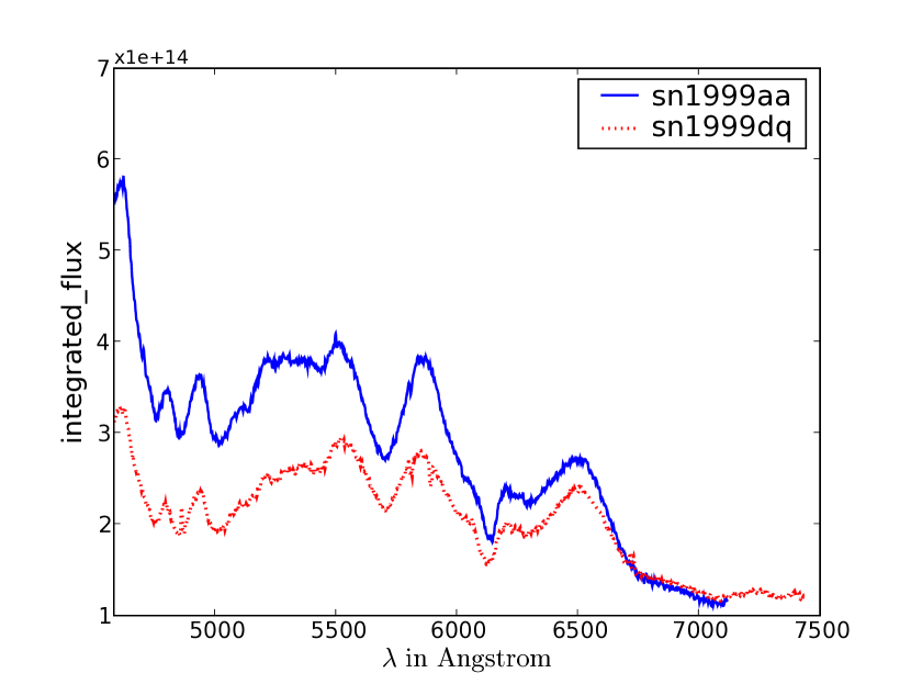
Figure 3.— This figure shows the spectra of SN 1999dq (solid blue line) and SN 1999aa (dotted red line). Note that the spectra of SN 1999aa and SN 1999dq have almost identical spectral features but that of SN 1999aa is warped toward the blue. This difference is most likely not real but an artifact of dereddening or background subtraction.

In order to avoid these problems, one has to do a very careful reduction and analysis to obtain the template SNe spectra.

• Interpolate the observed $B$ and $V$ light curves (no reddening corrections).

• Warp the spectra to match the observed $B-V$ color at a given epoch.

• Calculate the K-correction from the warped spectrum.

• Apply calculated K-corrections and deredden the $B$ and $V$ light curves to get the intrinsic $B-V$ color.

• Finally correct the spectrum by reddening and warping it to match the intrinsic color calculated from the light curve.

Similar techniques are being developed for SN Ia lightcurve fitting to get distances to SNe Ia. We are currently implementing these techniques and we will discuss their implementation in Rest et al. (2008).

3.2.2 Cross-Correlation of Spectra with SNID

One alternative to the $\chi^{2}$-minimization approach is the cross-correlation technique. In this paper, we use an implementation of the correlation techniques of Tonry & Davis (1979), the SuperNova IDentification code (SNID; Blondin & Tonry 2006, 2007). In SNID, the input and template spectra are binned on a common logarithmic wavelength scale, such that a redshift $(1+z)$ corresponds to a uniform linear shift in $\log\lambda$. The spectra are then “flattened” through division by a pseudo continuum, such that the correlation only relies on the relative shape and strength of spectral features, and is therefore insensitive to spectral color information (including reddening uncertainties and flux mis-calibrations). The pseudo-continuum is fitted as a 13-point cubic spline evenly spaced in log wavelength between 2500Åand 10000Å. We refer the reader to Blondin & Tonry (2007) where the SNID  algorithm is described in full detail. Finally, the spectra are smoothed by applying a bandpass filter to remove low-frequency residuals (wavelength scale $\gtrsim 300\rm{\AA}$) left over from the pseudo-continuum division and high-frequency noise (wavelength scale $\lesssim 50\rm{\AA}$) components. The main motivation for applying such a filter lies in the physical nature of supernova spectra, which are dominated by broad spectral lines ($\sim 100-150\rm{\AA}$) due to the large expansion velocities of the ejecta ($\sim 10000\rm{\hbox{$~{}$km$~{}$s${}^{-1}$}}$). A more detailed explanation of the spectrum pre-processing and cross-correlation in SNID  is given by Blondin & Tonry (2007).

The input spectrum is correlated in turn with each template spectrum. The redshift, $z$, is usually a free parameter in SNID  (indeed, this code was developed to determine the redshift of high-$z$ SN Ia spectra; Matheson et al. 2005; Miknaitis et al. 2007), but can be fixed when the redshift is known, as is the case here for the LMC ($z\approx 0.001$). The quality of a correlation is determined by the $rlap$ quality parameter, which is the product of the Tonry & Davis correlation height-noise ratio ($r$) and the spectrum overlap parameter ($lap$). $r$ is defined as the ratio of the height of the heighest peak in the correlation function to the root-mean-square of its antisymmetric component, while $lap$ is a measure of the overlap in restframe wavelength space between the input and template spectra (see Blondin & Tonry, 2007). For an input spectrum with the restframe wavelength range $[\lambda_{0},\lambda_{1}]$, $lap$ is in the range $0\leq lap\leq\ln(\lambda_{1}/\lambda_{0})$. In what follows, a “good” correlation corresponds to $rlap\geq 5$ with $lap\geq 0.4$ (Matheson et al., 2005; Miknaitis et al., 2007; Blondin & Tonry, 2006, 2007). Note that these limits are not derived from the dataset in this paper, but from comparing single epoch spectra from low and high-z SNe.

We correlate each pair of SN Ia spectra using the SNID terchniques in a similar fashion what we have done with the $\chi^{2}$-minimization. Figure 4 shows the $rlap$ values versus difference in ${\Delta m_{15}}$ of the SNID correlated Ia template spectra. There is a clear trend toward stronger correlation for spectra with similar ${\Delta m_{15}}$. Note that most of the pairs with $rlap\geq 10$ have a difference in ${\Delta m_{15}}$ of less than 0.25.

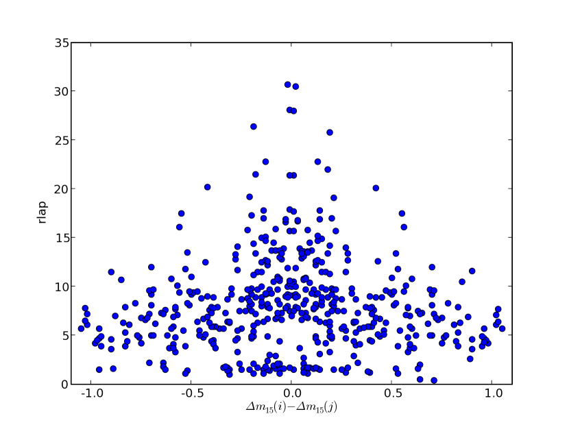
Figure 4.— This figure shows $rlap$ versus their difference in ${\Delta m_{15}}$: $\Delta m_{15}(i)-\Delta m_{15}(j)$ for all SN Ia in category $A$ and $B$. There is a clear trend toward stronger correlation for spectra with similar ${\Delta m_{15}}$.

The SNIDtechnique “flattens” the spectra before correlating them (see Section 3.2.2). The flattened spectra produced by SNID have the additional advantage that the $\chi^{2}$ is more robust against errors in dereddening or background subtraction. We calculate $\chi_{f}^{2}$ for all SN Ia pairs of flattened template spectra and plot it versus the difference in ${\Delta m_{15}}$ in Figure 5. The correlation between the goodness of fit indicated by $\chi_{f}^{2}$ and ${\Delta m_{15}}$ is significantly better than for $\chi^{2}$.

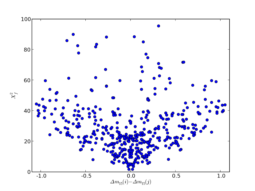
Figure 5.— This figure shows $\chi_{f}^{2}$ versus their difference in ${\Delta m_{15}}$: $\Delta m_{15}(i)-\Delta m_{15}(j)$ for all SN Ia in category $A$ and $B$. The correlation between the goodness of fit indicated by $\chi_{f}^{2}$ and ${\Delta m_{15}}$ is significantly better than for $\chi^{2}$.

We use the template spectra to test if $\chi_{f}^{2}$ can be used to determine the ${\Delta m_{15}}$: For a given SN Ia template spectra, we calculate the $\chi_{f}^{2}$ with respect to all other SN Ia templates. We find the template SNe with the smallest $\chi_{f}^{2}$ (noted $\chi^{2}_{f,min}$), and estimate the ${\Delta m_{15}}$ by computing the error-weighted mean ${\Delta m_{15}}$ for the three templates with the smallest $\chi_{f}^{2}\leq 2\times\chi^{2}_{f,min}$. Figure 6 shows the ${\Delta m_{15}}$ determined by the lightcurve shape versus the ${\Delta m_{15}}$ estimated using the $\chi_{f}^{2}$ (denoted as ${\Delta m_{15}}(\chi_{f}^{2})$. For SNe Ia with small ${\Delta m_{15}}\leq 1.1$, the agreement between true and estimated ${\Delta m_{15}}(\chi_{f}^{2})$ is excellent. However, for SNe Ia with ${\Delta m_{15}}>1.1$, there is a significant spread. The reason is that the sample of SN Ia with ${\Delta m_{15}}<1.1$ comprises both normal objects and overluminous ones with spectra similar to SN 1991T or SN 1999aa (Jeffery et al., 1992; Jha et al., 2006). These latter objects have spectra that show large deviations from normal SNe Ia, especially around maximum light (where the impact on the light-echo spectrum is the greatest). At intermediate ${\Delta m_{15}}$ ($1.2\lesssim{\Delta m_{15}}\lesssim 1.6$), however, SN Ia spectra are similar, and our approach does not enable a clear determination. The two points with large ${\Delta m_{15}}>1.8$ are both subluminous, 1991bg-like SNe Ia (Garnavich et al., 2004; Jha et al., 2006). The spectra show significant deviations from normal and overluminous SNe Ia around maximum light, yet the ${\Delta m_{15}}$ values are systematically underestimated. The disagreement is a simple consequence of the lack of 1991bg-like SN Ia in our set of spectral templates. With only two such templates with ${\Delta m_{15}}>1.6$ (see Table 1, the error-weighted mean ${\Delta m_{15}}$ of the three best-matching templates will systematically bias the ${\Delta m_{15}}$ determination to lower values. In Figure 7 we show the difference between the true ${\Delta m_{15}}$ and the estimated ${\Delta m_{15}}(\chi_{f}^{2})$ versus ${\Delta m_{15}}(\chi_{f}^{2})$. For ${\Delta m_{15}}(\chi_{f}^{2})\leq 1.1$, the standard deviation of the estimated ${\Delta m_{15}}(\chi_{f}^{2})$ compared to the true ${\Delta m_{15}}$ is 0.05 magnitudes. The calculated uncertainties of ${\Delta m_{15}}(\chi_{f}^{2})$ are slightly underestimated by a factor of 1.3. Therefore we consider ${\Delta m_{15}}(\chi_{f}^{2})$ as a very good estimate of the true ${\Delta m_{15}}$ for ${\Delta m_{15}}(\chi_{f}^{2})\leq 1.1$ with uncertainties smaller than 0.1 magnitudes. If the fitted ${\Delta m_{15}}>1.1$, then it can only be said that it is unlikely to be a 1991T-like SN Ia (1999cl is the only 91T-like SN Ia in our sample with ${\Delta m_{15}}>1.1$; see Table 1). More importantly, Figure 7 also shows that we are able to accurately determine the ${\Delta m_{15}}$ for SNe Ia with ${\Delta m_{15}}<1.1$. Since all 1991T-like SN Ia fulfill this condition, we are in principle able to not only determine the ${\Delta m_{15}}$ but also the SN Ia subtype for these objects. We will see in the next section that the light-echo spectrum presented here is most probably a 1991T-like SN Ia with $dm15<0.9$.

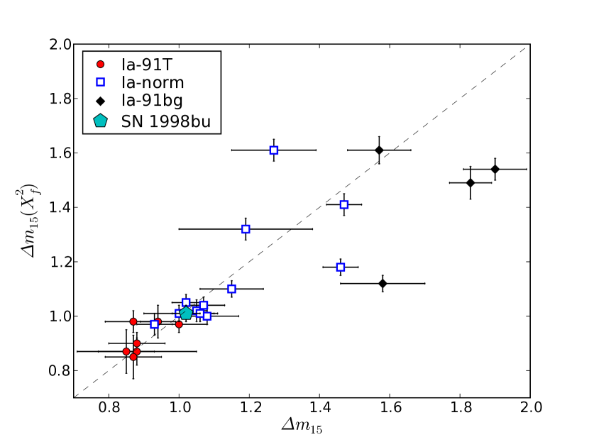
Figure 6.— This figure shows ${\Delta m_{15}}$ determined by the lightcurve shape versus the ${\Delta m_{15}}$ estimated using the $\chi_{f}^{2}$, denoted as ${\Delta m_{15}}(\chi_{f}^{2})$. The SN Ia subtypes “Ia-91T”, “Ia-norm”, and “Ia-91bg” are indicated with filled red circles, open blue squares, and filled black diamonds, respectively. The cyan pentagon inidicates SN 1998bu. For SNe Ia with small ${\Delta m_{15}}\leq 1.1$, the agreement between true and estimated ${\Delta m_{15}}(\chi_{f}^{2})$ is excellent. However, for SNe Ia with ${\Delta m_{15}}>1.1$, there is a significant spread.

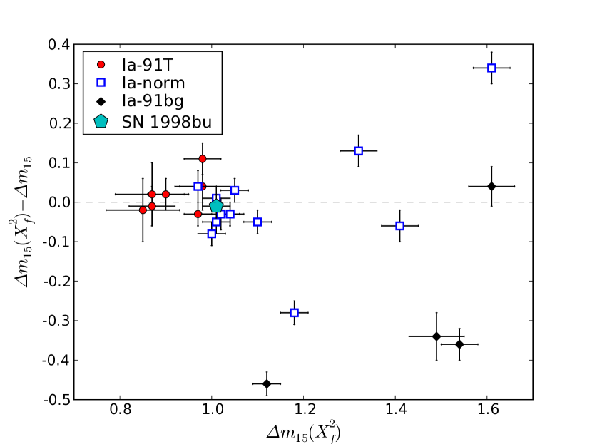
Figure 7.— This figure shows the difference between the true ${\Delta m_{15}}$ and the estimated ${\Delta m_{15}}(\chi_{f}^{2})$ versus ${\Delta m_{15}}(\chi_{f}^{2})$. The SN Ia subtypes “Ia-91T”, “Ia-norm”, and “Ia-91bg” are indicated with filled red circles, open blue squares, and filled black diamonds, respectively. The cyan pentagon inidicates SN 1998bu. For ${\Delta m_{15}}(\chi_{f}^{2})\leq 1.1$, the standard deviation of the estimated ${\Delta m_{15}}(\chi_{f}^{2})$ compared to the true ${\Delta m_{15}}$ is 0.05 magnitudes.

3.3. Single Scattering Approximation

Several authors have addressed the single scattering approximation for light echoes (Couderc, 1939; Chevalier, 1986; Emmering & Chevalier, 1989; Sugerman, 2003; Patat, 2005, e.g.). Following the derivation of Sugerman (2003), the surface brightness $B_{SC}$ of scattered light with wavelength $\lambda$ scattering at an angle $\theta$ off dust at position ${\bf r}$ and thickness $\Delta z$ is

$$B_{SC}(\lambda,\theta,{\bf r},\Delta z)=F(\lambda)n_{H}({\bf r})G({\bf r},\Delta z)S(\lambda,\theta)$$ (4)

Where $F(\lambda)$ is the time-integrated spectra of the SN, $n_{H}({\bf r})$ is the number density of hydrogen nuclei, $G({\bf r},\Delta z)$ is a geometrical factor depending on the geometry between the observer, SN, and dust, and the integrated scattering function $S(\lambda,\theta)$ which is described in more detail in Section 3.3.1.

Since for this paper we are only interested in the relative fluxes, we can drop all terms that are not dependent on the wavelength, add reddening by the LMC and MWG, and the modelled, observed spectrum $F_{scat}$ has the form

$$F_{scat}(\lambda)=C_{norm}C_{ext}^{MWG}(\lambda)C_{ext}^{LMC}(\lambda)F(\lambda)S(\lambda,\theta)$$ (5)

where $C_{ext}^{MWG}$, and $C_{ext}^{LMC}$ are the reddening by the MWG and the LMC, respectively, as discussed in Section 3.3.3.

3.3.1 Dust Properties

In order to get the total integrated scattering function $S(\lambda,\theta)$, we add up the integrated scattering function for each individual dust type:

$$S(\lambda,\theta)=\sum_{X}S_{X}(\lambda,\theta)$$ (6)

Following Weingartner & Draine (2001), $X$ can be $s$, $cn$, and $ci$ for silicon dust grains, carbonaceous dust grains with neutral PAH component, and carbonaceous dust grains with an ionized PAH component, respectively, where PAH stands for Polycyclic Aromatic Hydrocarbon. For a given dust type $X$, the integrated scattering function $S_{X}$ is

$$S_{X}(\lambda,\theta)=\int Q_{SC,X}(\lambda,a)\sigma_{g}\Phi_{X}(\theta,\lambda,a)f_{X}(a)da$$ (7)

where $Q_{SC,X}$ is the grain scattering efficiency, $\sigma_{g}=\pi a^{2}$ is the grain cross-section, $f_{X}(a)$ is the grain size distribution discussed in Section 3.3.2, and $\Phi_{X}(\theta,\lambda,a)$ is the Henyey & Greenstein (1941) phase function

$$\Phi_{X}(\lambda,\theta)=\frac{1-g_{X}^{2}(\lambda,a)}{(1+g_{X}^{2}(\lambda,a)-2g_{X}(\lambda,a)\cos{\theta})^{3/2}}$$ (8)

with $g(\lambda,a)$ the degree of forward scattering for a given grain. We integrate $S_{X}(\lambda,\theta)$ for the individual grain types by using the extended Simpson’s method (Press et al., 1992). We interpolate the values for $Q_{SC,X}$ and $g_{X}(\lambda,a)$ using the tables provided by B. T. Draine (Draine & Lee, 1984; Laor & Draine, 1993; Weingartner & Draine, 2001; Li & Draine, 2001).

3.3.2 Dust Grain Size Distribution

We use the models defined by Weingartner & Draine (2001) which consist of mixture of carbonaceous grains and amorphous silicate grains. Carbonaceous grains are PAH-like when small ($a\leq 10^{-3}\micron$), and graphite-like when large ($a>10^{-3}\micron$)(Li & Draine, 2001). The dust grain size distribution $f(a)$ is written as

$$f(a)\equiv\frac{1}{n_{H}}\frac{dn_{gr}}{da}$$ (9)

with $n_{gr}(a)$ is the number density of grains with size $\leq a$ and $n_{H}$ is the number density of H nuclei in both atoms and molecules. Weingartner & Draine (2001) derives the size distributions for different line of sights toward the LMC. We adopt the parameters of their “LMC avg” model and $b_{C}=2\times 10^{-5}$ (Table 3, Weingartner & Draine, 2001). We can then calculate the size distributions for carbonaceous dust $f_{ci}(a)=C_{ion}f(a)$ and $f_{cn}(a)=(1-C_{ion})f(a)$ using equations 2, 4, and 6 of Weingartner & Draine (2001). The PAH/graphitic grains are assumed to be 50% neutral and 50% ionized (Li & Draine, 2001), thus $C_{ion}=0.5$. For amorphous silicate dust $f_{s}$ we use equations 5 and 6.

3.3.3 Extinction

The extinction can be expressed as

$$\log_{10}C_{ext}(\lambda)=-0.4\langle A(\lambda)/A(V)\rangle R_{V}E(B-V)$$ (10)

For the MWG, we calculate the extinction $C_{ext}^{MWG}(\lambda)$ setting $R_{V}=3.1$ and $E_{MWG}(B-V)=0.07$, and by calculating $\langle A(\lambda)/A(V)\rangle$ using Equations 1-3 of Cardelli et al. (1989).

The average internal extinction of the LMC is $E(B-V)=0.1$ (Bessell, 1991), but different populations give different results. Zaritsky (1999) finds a mean $E(B-V)=0.06$ from red clump giants and $E(B-V)=0.14$ from OB types. They attribute this dependence to an age-dependent scale height: OB stars having a smaller scale height lie predominantly in the dusty disk. We use $E_{LMC}(B-V)=0.05$, half the average internal extinction value, since the most likely position of the SN is somewhere halfway through the LMC. Since the light echoes are not in the Superbubble of the LMC, we use the average $R_{V,LMC}=3.41$ value of the “LMC Average Sample” in Table 2, Gordon et al. (2003). Even though the extinction curves in the LMC and SMC have similarities to the MWG extinction curves, there are significant differences. Thus we calculate $\langle A(\lambda)/A(V)\rangle$ for the LMC using Equation 5 in Gordon et al. (2003) and the values in the “Average” row of the section “LMC Average Sample” in Table 3 in Gordon et al. (2003).

3.4. Testing the method with SN 1998bu

Several 100 days after the explosion, the light curve of the type Ia supernova SN 1998bu suddenly flattened. At the same time, the spectrum changed from the typical nebular emission to a blue continuum with broad absorption and emission features reminiscent of the SN spectrum at early phases (Cappellaro et al., 2001). This was explained by the emergence of a light echo from a foreground dust cloud. A similar case is SN 1991T, but its light echo spectra are of significantly less signal-to-noise.

We use SN 1998bu as a test cases to see if we can determine the ${\Delta m_{15}}$ of the SNe Ia from their light echo spectrum. We correlate the template spectra with the light echo spectrum and estimate with our method the ${\Delta m_{15}}(\chi_{f}^{2})$ of SN 1998bu. We can then compare how close this estimated ${\Delta m_{15}}$ is to the true, lightcurve measured ${\Delta m_{15}}=1.02\pm 0.04$. This is the ultimate test if the method works on a real world example.

For the light echo of SN 1998bu we assume that the reflecting dust is $z=70pc$ in front of the supernova, the host galaxy extinction is $A_{V}^{host}=0.86$, and $R_{V}=3.1$ (Cappellaro et al., 2001). Using these values, we can calculate time-integrated, dust scattered, and reddened template spectra by applying equation 5 for 28 SNe Ia, which we denote template spectra in what follows. As described in the previous Section 3.2.2, we calculate the $rlap$ and $\chi_{f}^{2}$ values using SNID for the observed light echo spectra with the spectra templates.

Figure 8 shows the $rlap$ values of the SN 1998bu light echo and the template spectra for the different SN Ia subtypes In general, 91T-like SNe Ia (filled red circles) have a lower than normal $\Delta m_{15}$ and are overluminous, slow decliners, whereas 91bg-like SNe Ia (filled black diamonds) have a large $\Delta m_{15}$ and are underluminous, fast decliners. Besides one outlier at ${\Delta m_{15}}=1.7$, all other $rlap\geq 5$ values are for SN Ia with ${\Delta m_{15}}<1.2$. This is in very good agreement with the ${\Delta m_{15}}=1.02\pm 0.04$ of SN 1998bu determined from its lightcurves (Note that the limit $rlap\geq 5$ is not derived from the dataset in this paper, but from comparing single epoch spectra from low and high-z SNe). Similarly, the best $\chi_{f}^{2}$ values are all for spectra templates with ${\Delta m_{15}}<1.2$ (see Figure 9). We apply our method to determine the ${\Delta m_{15}}$ described in Section 3.2.2 using the $\chi_{f}^{2}$ and estimate the ${\Delta m_{15}}(\chi_{f}^{2})=1.01\pm 0.03$ for SN 1998bu. This is within the errors to the ${\Delta m_{15}}$ determined with the lightcurves. Figure 6 and 7 show the ${\Delta m_{15}}(\chi_{f}^{2})$ of SN 1998bu (red circle). We find that the SNID correlation technique provides more than sufficient discrimination between input templates for ${\Delta m_{15}}\leq 1.1$

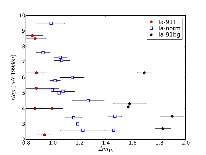
Figure 8.— Correlation parameter $rlap$ of the light echo of SN 1998bu determined with SNID versus $\Delta m_{15}$  of the time-integrated, dust-scattered, reddened, and flattened SN Ia spectra. The SN Ia subtypes “Ia-91T”, “Ia-norm”, and “Ia-91bg” are indicated with filled red circles, open blue squares, and filled black diamonds, respectively.

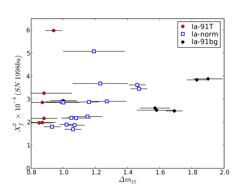
Figure 9.— $\chi_{f}^{2}$ versus $\Delta m_{15}$ for the fit of the time-integrated, dust-scattered, reddened, and flattened SN Ia spectra to the observed light echo spectrum associated with SN 1998bu. The SN Ia subtypes “Ia-91T”, “Ia-norm”, and “Ia-91bg” are indicated with filled red circles, open blue squares, and filled black diamonds, respectively.

4. Discussion

We have obtained a spectrum of the light echo located at RA=05:13:03.77 and DEC=-67:29:04.91 at epoch J2000. The associated SNR 0509-675 is at RA=05:09:31.922 and DEC=-67:31:17.12 at epoch J2000. The angular distance between the light echo and the SNR is 0.340 degrees. Using the SNR age of 400 years determined using light echo apparent motion (Rest et al., 2005b), we can determine the line-of-sight distance between the dust sheet and the SNR. We find this distance to be $z=300$ pc, which we use to calculate the scattering angle $\theta$. Then we can calculate the time-integrated, dust-scattered, and reddened template spectra by applying equation 5 for 28 SNe Ia and 6 SNe Ib/c. We use SNID to calculate the $rlap$ and $\chi_{f}^{2}$ using both the SNe Ia and SNe Ib/c templates (see Column (9) and (10) in Table 1 and Column (8) and (9) in Table 2).

The spectrum of the light echo associated with SNR 0509-675 shows broad emission and absorption features consistent with SN spectra. The question is, what kind of SN is it? Figure 10 shows the fit of two SN II template spectra (Type IIP and IIL) to the echo spectrum. Both spectra are created by using a spectral library by Nugent (Gilliland et al., 1999). The IIP spectra template is based mostly on the models seen in Baron et al. (2004), and its lightcurves are based on Cappellaro et al. (1997). There is no need for any sophisticated correlation or fitting technique to conclude that the observed light echo spectrum is not that of a Type II supernova.

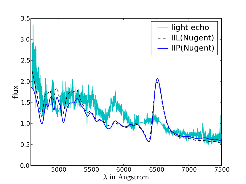
Figure 10.— Time-integrated, dust-scattered, and reddened SN II spectra fitted to the observed light echo spectrum (cyan line) associated with SNR 0509-675. The chip gaps (4838Å-4894Å, 6235Å-6315Å), and various LMC background emission lines ([O III], H$\alpha$, [N II], [S II]) are removed from the observed spectrum. The features do not correlate, and we conclude that the observed light echo spectrum is not a SN II spectrum.

Following the procedures described in Section 3.3 and 3.1, we have created the SN template spectra for 28 SNe Ia and 6 SNe Ib/c, and correlate these template spectra with the light echo spectrum using the SNID correlation technique described in Section 3.2.2. For the purpose of this paper, which is to identify the spectral (sub)type of the SN explosion that created SNR 0509-675, the SNID correlation technique described in Section 3.2.2 provides more than sufficient discrimination between input templates. This technique “flattens” both spectra, and then correlates the main features of the spectra. The strength of the correlation is reflected in the parameter $rlap$, with values of $rlap\geq 5.0$ indicating a strong correlation. Figure 11 shows the $rlap$ values versus $\Delta m_{15}$ of the SNID correlated Ia template spectra. The SN Ia subtypes “Ia-91T”, “Ia-norm”, and “Ia-91bg” are indicated with filled red circles, open blue squares, and filled black diamonds, respectively. There is an improved match with template spectra with smaller $\Delta m_{15}$ correlating more strongly with the observed light echo spectrum than the ones with large $\Delta m_{15}$. Only three templates, all with ${\Delta m_{15}}<0.9$, have a strong correlation with the observed light echo spectrum. Figure 12 shows a histogram of the $rlap$ values for the different SN Ia as well as Ib/c subtypes. Note that the normal SNe Ic (SN 1994I, SN 2004aw, SN 2005mf), denoted as “Ic-norm”, show stronger correlations than the other types of Ib/c (the broad-line SN Ic SN 1997ef, the peculiar SN Ib SN 2005bf, and the normal SN Ib SN 2005hg), denoted as “Ibc-other” in the lower panel of Figure 12 (see also Table 2). All SNe Ib/c have a significantly smaller $rlap$ value than three of the 91T-like SN Ia SN, and no SN Ib/c has an $rlap$ value bigger than 5, which is the cutoff value for a good correlation.

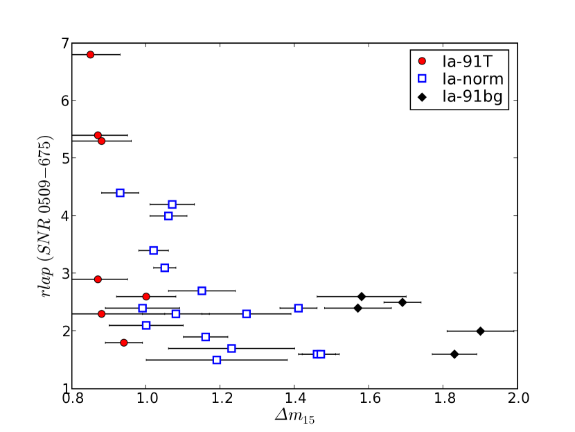
Figure 11.— Correlation parameter $rlap$ determined with SNID versus $\Delta m_{15}$  of the time-integrated, dust-scattered, reddened, and flattened SN Ia spectra. The SN Ia subtypes “Ia-91T”, “Ia-norm”, and “Ia-91bg” are indicated with filled red circles, open blue squares, and filled black diamonds, respectively. An $rlap$ value bigger than 5 is considered a strong correlation. There is a clear trend toward template spectra with small $\Delta m_{15}$ correlating stronger with the observed light echo spectrum than the ones with large $\Delta m_{15}$. Only three templates, all with ${\Delta m_{15}}<0.9$, have a strong correlation with the observed light echo spectrum ($rlap>5.0$).

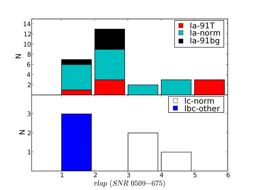
Figure 12.— Histogram of $rlap$ value determined with SNID for the different SN Ia subtypes (“Ia-91T”, “Ia-norm”, and “Ia-91bg”, upper panel), normal SN Ic type (“Ic-norm”, lower panel), and SN Ib/c type other than normal Ic (“Ibc-other”, lower panel). An $rlap$ value bigger than 5 indicates a good correlation between the two spectra. Note that the 91T-like SNe have the strongest correlation with the light echo spectrum. All SNe Ib/c have a significantly smaller $rlap$ value than three of the 91T-like SNe Ia, and no SNe Ib/c has an $rlap$ value bigger than 5, which is the cutoff value for a good correlation.

The flattened spectra produced by SNID have the additional advantage that the $\chi^{2}$ is more robust against errors in dereddening or background subtraction. We calculate $\chi_{f}^{2}$ of the flattened template spectra with respect to the flattened observed light echo spectra for all templates (see Column (9) in Table 1 and Column (8) in Table 2). Figure 13 shows $\chi_{f}^{2}$ versus $\Delta m_{15}$ for the different subtypes of SN Ia. The SN Ia subtypes “Ia-91T”, “Ia-norm”, and “Ia-91bg” are indicated with filled red circles, open blue squares, and filled black diamonds, respectively. The correlation between $\chi_{f}^{2}$ and $\Delta m_{15}$ is, as expected, excellent: The 5 SNe with the smallest $\chi_{f}^{2}$ also have the smallest $\Delta m_{15}$. This confirms that $rlap$ and $\chi^{2}$ are equally suitable measures of fit when the low spatial frequency feautures are removed. Figure 14 shows the histograms of $\chi_{f}^{2}$ for the different SN Ia subtypes (upper panel) and SN Ib/c subtypes (lower panel). Similar to the $rlap$ histograms, the normal SNe Ic have a decent $\chi_{f}^{2}$, but all 91T-like SNe with ${\Delta m_{15}}<0.9$ have a better $\chi_{f}^{2}$. We apply our method to determine the ${\Delta m_{15}}$ of the light echo spectra using the $\chi_{f}^{2}$, and we find that ${\Delta m_{15}}(\chi_{f}^{2})=0.87\pm 0.05$.

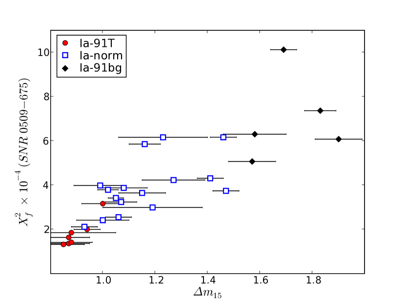
Figure 13.— $\chi_{f}^{2}$ versus $\Delta m_{15}$ for the fit of the time-integrated, dust-scattered, reddened, and flattened SN Ia spectra to the observed light echo spectrum associated with SNR 0509-675. The SN Ia subtypes “Ia-91T”, “Ia-norm”, and “Ia-91bg” are indicated with filled red circles, open blue squares, and filled black diamonds, respectively. The 5 SNe with the smallest $\chi_{f}^{2}$ are 91T-like SNe Ia and have the smallest $\Delta m_{15}$. Note that the goodness of fit correlates better with $\Delta m_{15}$ than subtype. The 91T-like SNe with comparably large $\Delta m_{15}$ have a larger $\chi_{f}^{2}$ than the normal Ia with small $\Delta m_{15}$.

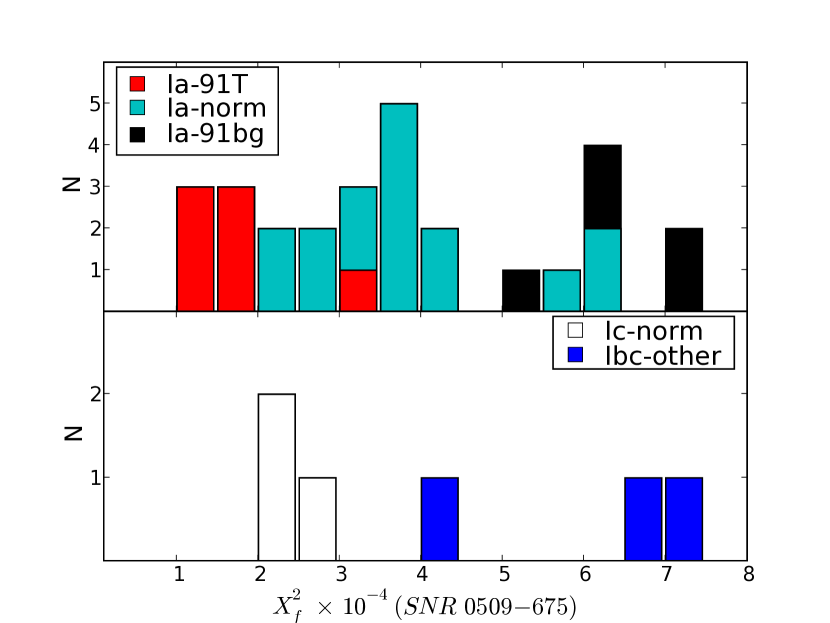
Figure 14.— The upper panel shows the histogram of $\chi_{f}^{2}$ for the fit of the time-integrated, dust-scattered, reddened, and flattened SN Ia spectra fit to the flattened observed light echo spectrum associated with SNR 0509-675. Note that nearly all 91T-like SNe Ia have a better $\chi_{f}^{2}$ than any SNe of the other subtypes. The lower panel shows the same histogram of $\chi_{f}^{2}$ for the SNe Ib/c. Note that the normal SNe Ic have a decent $\chi_{f}^{2}$, but all 91T-like SNe with ${\Delta m_{15}}<0.9$ have a better $\chi_{f}^{2}$.

Figure 15 shows the three 91T-like SN Ia template spectra with the best $rlap$ values, overplotted on the observed light echo spectrum. The template spectra have the same features than the observed light echo spectrum, and that the agreement is very good. The only significant disagreement is that the template spectra have a slightly deeper absorption and stronger emission at $6100$Å and $6500$Å, respectively. The two “normal” SNe Ia with the best $rlap$ values are very similar and fit as well very good for wavelength smaller than $5800$Å, but the difference in strength of the two features at $6100$Å and $6500$Åis more pronounced (see Figure 16). Note also that these two best-correlating normal SNe Ia are also the ones with the smallest $\Delta m_{15}$ values. Figure 17 shows the three SN Ib/c template spectra with the best $rlap$ values. Even though there are similarities between the template spectra and the observed spectrum, the relative strength of the spectral features is not as consistent as for the SNe Ia. A few examples of SN template spectra with a poor correlation to the observed light echo spectrum are shown in Figure 18.

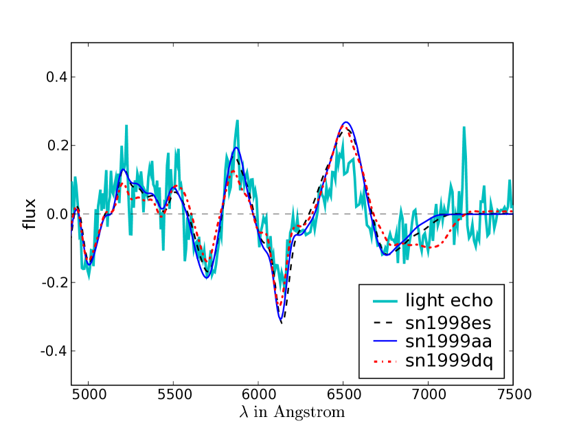
Figure 15.— The three time-integrated, dust-scattered, reddened, and flattened SN Ia spectra with the best $rlap$ values (i.e. the best correlation with the observed light echo spectrum), overplotted on the flattened observed light echo spectrum (solid cyan line). Note that all three template spectra are 91T-like SNe Ia with ${\Delta m_{15}}<0.9$.

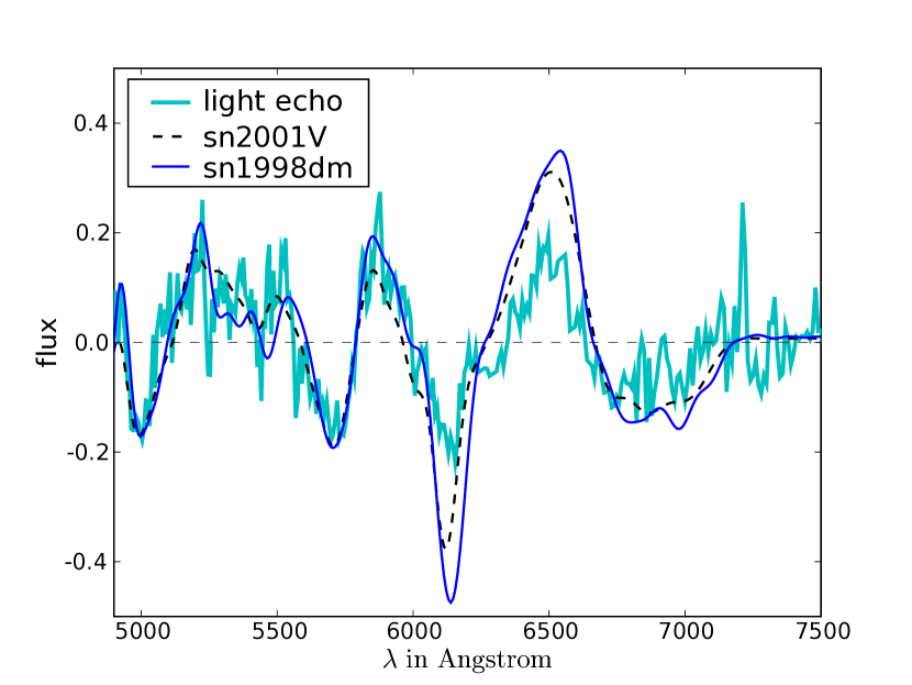
Figure 16.— The two time-integrated, dust-scattered, reddened, and flattened spectra of normal SNe Ia with the best rlap values, overplotted on the flattened observed light echo spectrum (solid cyan line). Note that these two template spectra are also the two normal SNe Ia with the smallest $\Delta m_{15}$.

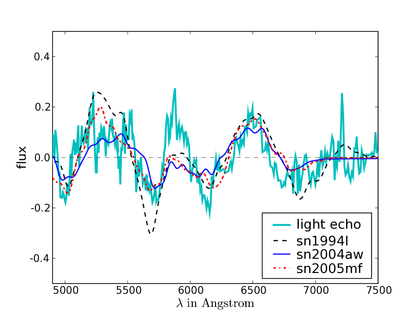
Figure 17.— The three time-integrated, dust-scattered, reddened, and flattened SN Ib/c spectra with the best $rlap$ values, overplotted on the flattened observed light echo spectrum (solid cyan line). Note that all three template spectra are normal SNe Ic.

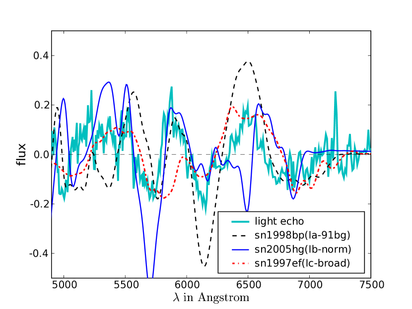
Figure 18.— Three time-integrated, dust-scattered, reddened, and flattened SN template spectra of different types having a bad correlation with the observed light echo spectrum (cyan line).

We conclude that the SN that created SNR 0509-675 is a 91T-like SN with ${\Delta m_{15}}<0.9$. Knowing the SN type (and moreover its subtype and thus how energetic the explosion was) places stringent constraints on the explosion mechanism and hence on the interpretation of X-ray spectra of the remnant. Analysis of X-ray data of SNR 0509-675 by Hughes et al. (1995) classifies this SNR as a remnant of a SN Ia. Recent analysis of X-ray spectra by Badenes & Bravo (2008) also supports the classification as an overluminous, 91T-like SN Ia: models using hydrodynamic calculations and nonequilibrium ionization simulations of highly energetic SN Ia reproduce the X-ray spectrum with its line flux ratios better than normal or subenergetic models (Badenes & Bravo, 2008). This is the first time that the (sub)type of an ancient SN has been determined by direct means by taking the spectrum of the original event.

5. Conclusions

We have obtained a spectrum of a light echo associated with SNR 0509-675. By comparing and correlating time-integrated, dust-scattered, and reddened template spectra created from a spectral library of nearby supernovae of all types to the light echo spectrum, we find that overluminous, 91T-like SNe Ia match the observed spectrum best. We correlate the template spectra with the observed spectra with SNID. The correlation parameter $rlap$ is a measure of the strength of the correlation, and $rlap\geq 5$ indicates a strong correlation. Only SN Ia with ${\Delta m_{15}}<0.9$ pass this cut. They correspond to intrinsically overluminous SNe Ia with a spectrum resembling the prototypical SN 1991T (Jeffery et al., 1992). Similarly, all 91T-like SN Ia with ${\Delta m_{15}}<0.9$ have a smaller $\chi^{2}$ than any other SNe when the “flattened” (see Section 3.2.2) SN templates are fitted to the observed spectrum. Normal SNe Ic show some similarities to the observed light echo spectrum. However, the correlation is only weak ($rlap<5$) and their $\chi^{2}$ is larger than the $\chi^{2}$ of the 91T-like SN Ia. Thus we can exclude them as the possible source event for SNR 0509-675. This is the first time that the (sub)type of a SN is conclusively and directly determined long after the event happened. Light echoes provide an excellent opportunity to connect the physics of the SN itself to its remnant. Much can be learned about the physics of SNe and their impact on the surrounding ISM from this direct comparison: Knowing the SN type (and moreover its subtype and thus how energetic the explosion was) places stringent constraints on the explosion mechanism and hence on the interpretation of X-ray spectra of the remnant (Badenes & Bravo, 2008). For the first time, models of SN explosions can now be tested for their mutual conistency with the SNe explosion itself and the observations of the SNR. We are currently working on expanding the sample of SNR with light echo spectra: In the LMC alone there are two more SNR with associated light echoes. Our investigation suggests also that subtyping of historical Milky Way supernovae, particularly the more recent SN 1572 (Tycho), SN 1604 (Kepler) and Cas A events, should be possible provided that suitable light echo features are found and can be studied spectroscopically. Such a sample of SNRs with known explosion spectra will place stringent constrains on SNe explosion models and enhance our understanding of these events that play such an important role in the production of heavy elements in our universe.

6. Acknowledgments

Based on observations obtained for programs GS-2005B-Q-11 and GS-2006B-Q-41 at which is operated by the Association of Universities for Research in Astronomy, Inc., under a cooperative agreement with the NSF on behalf of the Gemini partnership: the National Science Foundation (United States), the Science and Technology Facilities Council (United Kingdom), the National Research Council (Canada), CONICYT (Chile), the Australian Research Council (Australia), CNP (Brazil) and CONICEI (Argentina). The SuperMACHO survey was conducted under the auspices of the NOAO Survey Program. The support of the McDonnell Foundation, through a Centennial Fellowship awarded to C. Stubbs, has been essential to the SuperMACHO survey. AR thanks the Goldberg Fellowship Program for its support. DW acknowledges the support of a Discovery Grant from the Natural Sciences and Engineering Research Council of Canada (NSERC). AC is supported by FONDECYT grant 1051061. AG thanks the University of Washington Department of Astronomy for facilities support. DM, GP, LM and AC are supported by Fondap Center for Astrophysics 15010003. The work of MH, KHC and SN was performed under the auspices of the U.S. Department of Energy by Lawrence Livermore National Laboratory in part under Contract W-7405-Eng-48 and in part under Contract DE-AC52-07NA27344. MWV is supported by AST-0607485. GP acknowledges support by the Proyecto FONDECYT 3070034. We thank Geoffrey C. Clayton for fruitful discussions on how to implement the LMC internal reddening. This research has made use of the CfA Supernova Archive, which is funded in part by the National Science Foundation through grant AST 0606772.

Table 1

SN	Subtype	$\Delta m_{15}$	N	$p_{min}$	$p_{max}$	$w_{max}$	Grade	$\chi^{2}_{f}*10^{-4}$	rlap
(1)	(2)	(3)	(4)	(5)	(6)	(7)	(8)	(9)	(10)
sn1991T	Ia-91T	$0.94\pm 0.05$	18	-15.50	71.50	0.2041	A	2.00	1.8
sn1992A	Ia-norm	$1.47\pm 0.05$	11	-7.50	25.50	0.2087	A	3.74	1.6
sn1997do	Ia-norm	$0.99\pm 0.10$	12	-12.05	20.79	0.2878	B	3.98	2.4
sn1998V	Ia-norm	$1.06\pm 0.05$	8	-1.99	41.99	0.3026	B	2.55	4.0
sn1998ab	Ia-91T	$0.88\pm 0.17$	10	-8.13	46.74	0.4090	C	1.85	2.3
sn1998aq	Ia-norm	$1.05\pm 0.03$	14	-1.24	48.67	0.2990	B	3.42	3.1
sn1998bp	Ia-91bg	$1.83\pm 0.06$	11	-5.03	27.85	0.2189	A	7.37	1.6
sn1998bu	Ia-norm	$1.02\pm 0.04$	26	-3.36	43.66	0.2159	A	3.79	3.4
sn1998dh	Ia-norm	$1.23\pm 0.17$	10	-10.07	44.82	0.4386	C	6.16	1.7
sn1998dm	Ia-norm	$1.07\pm 0.06$	10	2.91	45.86	0.4007	C	3.24	4.2
sn1998ec	Ia-norm	$1.08\pm 0.09$	6	-3.98	39.01	0.2545	B	3.88	2.3
sn1998eg	Ia-norm	$1.15\pm 0.09$	6	-0.35	23.68	0.3581	C	3.65	2.7
sn1998es	Ia-91T	$0.87\pm 0.08$	20	-12.28	43.72	0.1753	A	1.36	5.4
sn1999aa	Ia-91T	$0.85\pm 0.08$	22	-11.16	47.64	0.2044	A	1.32	6.8
sn1999ac	Ia-91T	$1.00\pm 0.08$	16	-5.97	38.96	0.1817	A	3.16	2.6
sn1999by	Ia-91bg	$1.90\pm 0.09$	13	-5.36	40.67	0.1568	A	6.08	2.0
sn1999cc	Ia-norm	$1.46\pm 0.05$	7	-4.14	24.82	0.2495	A	6.17	1.6
sn1999cl	Ia-91T	$1.19\pm 0.19$	11	-9.32	36.67	0.2792	B	2.99	1.5
sn1999dq	Ia-91T	$0.88\pm 0.08$	21	-13.02	45.84	0.1597	A	1.41	5.3
sn1999ej	Ia-norm	$1.41\pm 0.05$	5	-2.23	10.76	0.4068	C	4.31	2.4
sn1999gd	Ia-norm	$1.16\pm 0.06$	5	0.02	33.89	0.4036	C	5.86	1.9
sn1999gh	Ia-91bg	$1.69\pm 0.05$	12	2.02	38.88	0.4359	C	10.12	2.5
sn1999gp	Ia-91T	$0.87\pm 0.08$	8	-6.29	34.62	0.1947	A	1.64	2.9
sn2000cf	Ia-norm	$1.27\pm 0.12$	6	-0.16	22.83	0.3560	C	4.23	2.3
sn2000cn	Ia-91bg	$1.58\pm 0.12$	9	-10.14	26.77	0.2764	B	6.30	2.6
sn2000dk	Ia-91bg	$1.57\pm 0.09$	6	-5.11	33.77	0.2575	B	5.07	2.4
sn2000fa	Ia-norm	$1.00\pm 0.10$	13	-12.03	41.68	0.1623	A	2.42	2.1
sn2001V	Ia-norm	$0.93\pm 0.05$	28	-15.50	48.50	0.2020	A	2.12	4.4

Note. — Overview of SN Ia template spectra(Matheson, 2007). Column (1) shows the SN identifier. Column (2) shows the SN Ia subtype, where “Ia-91T” indicate the overluminous, slow decliners, “Ia-norm” are the “normal” SN Ia, and “Ia-91bg” are the underluminous, fast decliners. Column (3) shows the $\Delta m_{15}$ of the SN Ia. The number of spectra $N$ are shown in Column (4), spanning a phase from $p_{min}$ to $p_{min}$ days (Column (5) and (6)) with respect to the fitted $V$-band peak. Based on $w_{max}$ in Column (7) (The biggest weight assigned to a the spectra for a given SNe), a grade $A$, $B$, or $C$ is assigned to each SNe (Column (8)), as described in Section 3.1. The $\chi^{2}_{f}$ for the fit of the time-integrated, dust-scattered, reddened, and flattened SN Ia spectra to the observed light echo spectrum is shown in Column (9). Column (10) shows the $rlap$ value determined with SNID indicating the correlation between the SN template and the observed light echo spectrum. An $rlap$ value bigger than 5 is considered a good correlation.

Table 2

SN	Subtype	N	$p_{min}$	$p_{max}$	$w_{max}$	Grade	$\chi^{2}_{f}*10^{-4}$	rlap	Ref.
(1)	(2)	(3)	(4)	(5)	(6)	(7)	(8)	(9)	(10)
sn1994I	Ic-norm	18	-6.50	63.50	0.2703	B	2.90	3.8	Filippenko et al. (1995)
sn1997ef	Ic-broad	25	-12.50	82.50	0.1485	A	4.08	1.1	Iwamoto et al. (2000)
sn2004aw	Ic-norm	25	-7.50	46.50	0.1610	A	2.17	3.7	Taubenberger et al. (2006)
sn2005bf	Ib-pec	22	-28.50	33.50	0.1474	A	6.68	1.0	Modjaz (2007)
sn2005hg	Ib-norm	16	-13.50	26.50	0.3285	B	7.45	1.0	Modjaz (2007)
sn2005mf	Ic-norm	4	3.50	13.50	0.4233	C	2.02	4.2	Modjaz (2007)

Note. — Same as Table 1, but with no $\Delta m_{15}$ column, Column (2) shows the subtypes of SN Ib/c, and Column (10) shows the reference of the SN data.

References

- Badenes & Bravo (2008) Badenes, H. J. P. C. G., C., & Bravo, E. 2008, ApJ, in press
- Baron et al. (2004) Baron, E., Nugent, P. E., Branch, D., & Hauschildt, P. H. 2004, ApJ, 616, L91
- Bessell (1991) Bessell, M. S. 1991, A&A, 242, L17
- Bessell (1999) Bessell, M. S. 1999, PASP, 111, 1426
- Blondin & Tonry (2006) Blondin, S., & Tonry, J. L. 2006, in ”The Multicoloured Landscape of Compact Objects and their Explosive Progenitors: Theory vs Observations” (Cefalu, Sicily, June 2006). Eds. L. Burderi et al. (New York: AIP)
- Blondin & Tonry (2007) Blondin, S., & Tonry, J. L. 2007, accepted for publication in ApJ, 666, 1024
- Boffi et al. (1999) Boffi, F. R., Sparks, W. B., & Macchetto, F. D. 1999, A&AS, 138, 253
- Bond et al. (2003) Bond, H. E., et al. 2003, Nature, 422, 405
- Cappellaro et al. (2001) Cappellaro, E., et al. 2001, ApJ, 549, L215
- Cappellaro et al. (1997) Cappellaro, E., Turatto, M., Tsvetkov, D. Y., Bartunov, O. S., Pollas, C., Evans, R., & Hamuy, M. 1997, A&A, 322, 431
- Cardelli et al. (1989) Cardelli, J. A., Clayton, G. C., & Mathis, J. S. 1989, ApJ, 345, 245
- Chevalier (1986) Chevalier, R. A. 1986, ApJ, 308, 225
- Couderc (1939) Couderc, P. 1939, Annales d’Astrophysique, 2, 271
- Crotts (1988) Crotts, A. 1988, IAU Circ., 4561, 4
- Draine & Lee (1984) Draine, B. T., & Lee, H. M. 1984, ApJ, 285, 89
- Emmering & Chevalier (1989) Emmering, R. T., & Chevalier, R. A. 1989, ApJ, 338, 388
- Filippenko et al. (1995) Filippenko, A. V., et al. 1995, ApJ, 450, L11
- Garg et al. (2007) Garg, A., et al. 2007, AJ, 133, 403
- Garnavich et al. (2004) Garnavich, P. M., et al. 2004, ApJ, 613, 1120
- Gilliland et al. (1999) Gilliland, R. L., Nugent, P. E., & Phillips, M. M. 1999, ApJ, 521, 30
- Glazebrook & Bland-Hawthorn (2001) Glazebrook, K., & Bland-Hawthorn, J. 2001, PASP, 113, 197
- Gordon et al. (2003) Gordon, K. D., Clayton, G. C., Misselt, K. A., Landolt, A. U., & Wolff, M. J. 2003, ApJ, 594, 279
- Hamuy et al. (1994) Hamuy, M., Suntzeff, N. B., Heathcote, S. R., Walker, A. R., Gigoux, P., & Phillips, M. M. 1994, PASP, 106, 566
- Hamuy et al. (1992) Hamuy, M., Walker, A. R., Suntzeff, N. B., Gigoux, P., Heathcote, S. R., & Phillips, M. M. 1992, PASP, 104, 533
- Henyey & Greenstein (1941) Henyey, L. G., & Greenstein, J. L. 1941, ApJ, 93, 70
- Hughes et al. (1995) Hughes, J. P., et al. 1995, ApJ, 444, L81
- Iwamoto et al. (2000) Iwamoto, K., et al. 2000, ApJ, 534, 660
- Jeffery et al. (1992) Jeffery, D. J., Leibundgut, B., Kirshner, R. P., Benetti, S., Branch, D., & Sonneborn, G. 1992, ApJ, 397, 304
- Jha et al. (2006) Jha, S., et al. 2006, AJ, 131, 527
- Kapteyn (1902) Kapteyn, J. C. 1902, Astronomische Nachrichten, 157, 201
- Laor & Draine (1993) Laor, A., & Draine, B. T. 1993, ApJ, 402, 441
- Li & Draine (2001) Li, A., & Draine, B. T. 2001, ApJ, 554, 778
- Liu et al. (2003) Liu, J.-F., Bregman, J. N., & Seitzer, P. 2003, ApJ, 582, 919
- Matheson (2007) Matheson, T. 2007, in preparation
- Matheson et al. (2005) Matheson, T., et al. 2005, AJ, 129, 2352
- Matheson et al. (2000) Matheson, T., Filippenko, A. V., Ho, L. C., Barth, A. J., & Leonard, D. C. 2000, AJ, 120, 1499
- Miknaitis et al. (2007) Miknaitis, G., et al. 2007, ApJ, 666
- Modjaz (2007) Modjaz, M. 2007, Ph.D. thesis, AA(Harvard University)
- Newman & Rest (2006) Newman, A. B., & Rest, A. 2006, PASP, 118, 1484
- Patat (2005) Patat, F. 2005, MNRAS, 357, 1161
- Patat et al. (2006) Patat, F., Benetti, S., Cappellaro, E., & Turatto, M. 2006, MNRAS, 369, 1949
- Press et al. (1992) Press, W. H., Teukolsky, S. A., Vetterling, W. T., & Flannery, B. P. 1992, Numerical recipes in C. The art of scientific computing (Cambridge: University Press, —c1992, 2nd ed.)
- Prieto et al. (2006) Prieto, J. L., Rest, A., & Suntzeff, N. B. 2006, ApJ, 647, 501
- Quinn et al. (2006) Quinn, J. L., Garnavich, P. M., Li, W., Panagia, N., Riess, A., Schmidt, B. P., & Della Valle, M. 2006, ApJ, 652, 512
- Rest et al. (2008) Rest, A., Foley, R., Matheson, T., & Blondin, S. 2008, AJ, in preparation
- Rest et al. (2005a) Rest, A., et al. 2005a, ApJ, 634, 1103
- Rest et al. (2005b) Rest, A., et al. 2005b, Nature, 438, 1132
- Ritchey (1901a) Ritchey, G. W. 1901a, ApJ, 14, 293
- Ritchey (1901b) Ritchey, G. W. 1901b, ApJ, 14, 167
- Ritchey (1902) Ritchey, G. W. 1902, ApJ, 15, 129
- Schaefer (1988) Schaefer, B. E. 1988, ApJ, 327, 347
- Schmidt et al. (1994) Schmidt, B. P., Kirshner, R. P., Leibundgut, B., Wells, L. A., Porter, A. C., Ruiz-Lapuente, P., Challis, P., & Filippenko, A. V. 1994, ApJ, 434, L19
- Shklovskii (1964) Shklovskii, I. S. 1964, Astron. Circ. USSR, 306
- Sparks et al. (1999) Sparks, W. B., Macchetto, F., Panagia, N., Boffi, F. R., Branch, D., Hazen, M. L., & della Valle, M. 1999, ApJ, 523, 585
- Sugerman (2003) Sugerman, B. E. K. 2003, AJ, 126, 1939
- Sugerman (2005) Sugerman, B. E. K. 2005, ApJ, 632, L17
- Sugerman & Crotts (2002) Sugerman, B. E. K., & Crotts, A. P. S. 2002, ApJ, 581, L97
- Suntzeff et al. (1988) Suntzeff, N. B., Heathcote, S., Weller, W. G., Caldwell, N., & Huchra, J. P. 1988, Nature, 334, 135
- Swope (1940) Swope, H. H. 1940, Harvard College Observatory Bulletin, 913, 11
- Taubenberger et al. (2006) Taubenberger, S., et al. 2006, MNRAS, 371, 1459
- Tonry & Davis (1979) Tonry, J., & Davis, M. 1979, AJ, 84, 1511
- van den Bergh (1965) van den Bergh, S. 1965, PASP, 77, 269
- van den Bergh (1966) van den Bergh, S. 1966, PASP, 78, 74
- van den Bergh (1975) van den Bergh, S. 1975, Ap&SS, 38, 447
- van den Bergh (1977) van den Bergh, S. 1977, PASP, 89, 637
- Van Dyk et al. (2006) Van Dyk, S. D., Li, W., & Filippenko, A. V. 2006, PASP, 118, 351
- Wade & Horne (1988) Wade, R. A., & Horne, K. 1988, ApJ, 324, 411
- Weingartner & Draine (2001) Weingartner, J. C., & Draine, B. T. 2001, ApJ, 548, 296
- Welch (2007) Welch, D. L. 2007, ApJ, 669, 525
- Zaritsky (1999) Zaritsky, D. 1999, AJ, 118, 2824