Exploring Urban Environments
By Random Walks

Abstract

A complex web of roads, walkways and public transport systems can hide areas of geographical isolation very difficult to analyze. Random walks are used to spot the structural details of urban fabric.

To Ludwig Streit on his $70^{th}$ birthday with warm wishes

PACS: 89.65.Lm, 89.75.Fb, 05.40.Fb, 02.10.Ox

Keywords: Space syntax, Queuing networks, Random walks

1 Introduction

In the present paper, we discuss the application of Markov processes to urban studies. However, it is important to emphasize that the approach related to Markov processes (such as random walks) can be used to analyze any type of complex networks. The main technical idea beyond the method is to investigate the properties of networks by exploiting the spectral properties of self-adjoint operators (symmetric matrices) defined on their graph representations. It is then obvious that a network can be effectively investigated by spectral methods, if it is not too large. The spatial networks of human settlements give good examples - for instance, the city of Paris (inside the Periphery Boulevard) contains only 5131 interconnected open spaces.

A city converts a space pattern into a pattern of relationships. While discussing the impact a spatial structure has on the social establishment, it is inevitable to mention two Englishmen. After the British House of Commons had been destroyed in 1941, a long debate commenced in the Parliament on whether the old House insufficient to seat for all of its members be rebuilt or a new modern House should be constructed. In his speech to the meeting in the House of Lords, October 28, 1943, Sir Winston Churchill exclaimed, ”We shape our buildings, and afterwards our buildings shape us” [1], as if he believed that the movement pattern emerged in the old House of Common is responsible for the establishing and sustain of the British political tradition. This intuitive knowledge had been conceived by another British gentleman, Bill Hillier, professor at University College of London, within the concept of space syntax, a theory developed in the late 1970s, that seeks to reveal the mutual effects of complex spatial urban networks on society and vice versa [2, 3]. The joint use of scarce space by many people creates life in cities which is driven largely by micro-economic factors which are invariant over various cultures that tends to give cities similar structures. Hereby, the street configuration itself naturally creates differential patterns of occupancy (as an emergent phenomenon), whereby some streets become, over time, more highly used than others [4]. At the same time, a background residential space process driven by cultural factors tend to make cities different from each other, so that the emergent urban grid pattern containing an imprint of certain geometrical regularities forms a network of interconnected open spaces, being a historical record of a city creating process driven by human activity and containing traces of society and history [2].

It is important to note that from the very beginning, graph theory had been developed in a close relation to urban studies: Leonard Euler’s founding paper on the Seven Bridges of Königsberg published in 1736 is regarded as the first paper in the history of graph theory, [5]. In the present paper, we review the spectral algorithms designed to analyze transport networks. In particular, the method proves its efficiency for revealing the disadvantageous areas designed to foster crime, deprivation, and ghettoisation, [6].

In the forthcoming sections, we explain that city space syntax can be considered as a queuing network operating in the free flow regime (see Sec. 2). The steady state of a queuing network (see Sec. 2.1) is determined by the set of automorphisms of the graph spanning the network (Sec. 2.2). We shall show that these automorphisms naturally correspond to random walks of the nearest neighboring type, in which a traveller, after passing through an open space, randomly chooses another space to move in among those intersecting with the given one. How many possibilities to move the walker has while in an arbitrary place? - Indeed, it depends upon the type of the city he dwells in. We have analyzed two German medieval organic cities, the city canal network in Venice, and the regular street grid in Manhattan and found that while the organic towns are relatively compact (the majority of streets in them are just three steps apart from each other), the bigger urban patterns demonstrate the structure of small worlds, in which a dense network of relatively short local streets is supported by the long axial itineraries connecting the far-away districts within the city that essentially simplifies the navigation and transportation tasks in the urban environment (see Sec. 3). Being a representation of the set of graph automorphisms, random walks provide us with an effective tool for describing the graph structure in details (see Sec. 4, 5). In Sec. 6, we illustrate the method by studying two graphs by random walks. The first graph is the regular Petersen graph which contains just 10 nodes, and we investigate the network of Venetian 96 canals as the second example.

The term ”random walk” was originally proposed by K. Pearson in 1905 in his letter to Nature devoted to a simple model describing a mosquito infestation in a forest: at each time step, a single mosquito moves a fixed length, at a randomly chosen angle (see [7]). Nowadays it is well known that random walks could be effectively used in order to investigate and characterize how effectively the nodes and edges of large networks can be covered by different strategies, [8, 9, 10]. Random walks help us to explore the structural properties of complex urban networks which cannot be detected by the usual methods designed primarily to unravel the structures of large quasi-random graphs. We conclude in the last section (Sec.7).

2 City space syntax as a queueing network with a steady-state behavior

Any graph representation naturally arises as the outcome of a categorization, when we abstract a real world system by eliminating all but one of its features and by grouping together items (or places) sharing a common attribute. For instance, the common attribute of all open spaces in city space syntax is that we can move through them. All elements called nodes that fall into one and the same set $V$ are considered as essentially identical; permutations of them within $V$ are of no consequence. The symmetric group $\mathbb{S}_{N}$ consisting of all permutations of $N$ elements ($N$ being the cardinality of the set $V$) constitute therefore the symmetry group of $V$. If we denote by $E\subseteq V\times V$ the set of ordered pairs of nodes called edges, then a graph is a map $G(V,E):E\to K\subseteq\mathbb{R}_{\,+}$. We suppose that the graph is undirected and has no multiple edges. If two nodes are adjacent, $(i,j)\in E$, we write $i\sim j$. The degree of the node $i\in V$ is the number of its neighbors in $G$, $\deg_{G}(i)=k_{i}$.

The set of interconnected urban open spaces in which a pedestrian or a vehicle, upon departures from one space, can join another constitutes a queueing network that can be regarded as a graph whose nodes represent the open spaces (streets, squares, and round-abouts), and whose edges represent links between nodes (junctions and crossroads). In the queueing theory [11], the paths along which a traveller may move from service station to service station are determined by the routing probabilities, and then the theory of Markov chains provides the statistical models for the analysis of queueing networks. Travellers arriving to an open space are either moving through it immediately or queuing until the space becomes available. Once the space is passed through, the traveller is routed to its next station, which is chosen according to a probability distribution among all other open spaces linked to the given one in the city. However, if the destination space has finite capacity then it may be full and then the traveller will be blocked at its current location until the next space becomes available.

2.1 Steady states in queuing networks

If the network of $N$ open spaces is not at all congested (as long as inflows are compatible with system capacities), there is a network flow - say, cars are travelling through it at some constant speed $v>0$ in the free flow regime. Given $\left(X_{t}:t\geq 0\right)$, a i.i.d. random process characterized by some distribution $f$ defined on $V$ and let $p_{i}>0$ be the arrival probability at the node $i\in V$, in a sequence of $n$ independent Bernoulli trials, then travellers visit the node $i$ in average $np_{i}$ times. If trials are conducted in a finite time interval $t$, during which events occur in sequence, we denote the proportion of time spent by a traveller in $i$ by $\lambda_{i}>0,$

$$np_{i}\,=\,\lambda_{i}t,$$ (1)

The above formula expresses the linear Ohm’s law relating the time variable with the number of independent Bernoulli trials, $t=(p_{i}/\lambda_{i})n$.

Assuming the Kirchoff’s current law, i.e. the total flow into any node equals the flow out, then the proportions $\lambda_{i}$ can be obtained as the solutions of the global balance equations (transport equations) satisfying a normalization condition,

$$\sum_{i\in V}\,\lambda_{i}\,=\,1.$$ (2)

In the queuing network load in the stationary regime with free flow, the steady states (or densities) $\lambda_{i}>0$ can be interpreted as the length distances of the correspondent streets $i\in V$ normalized by (2).

In relation to a given distribution of $\lambda_{i}$, there are several ”performance indicators” characterizing the transport properties of the queuing network with respect to the random process $\left(X_{t}:t\geq 0\right)$. Given the arrival probability $p_{i}=t\lambda_{i}/n$, no matter from which node $X_{t=0}=j$ the process starts, the first arrival probability (FAP) that a traveller arrives at the node $i\in V$ by time $t^{\prime}>t$ is given by $P\left(\left.t^{\prime}>t\,\right|X_{t^{\prime}}=i\right)\,=\,\left(1-t\cdot\lambda_{i}/n\right)^{n}.$ First encounter properties estimated by random walks play a crucial role in explorations of various real-world networks, including epidemic spreading, transport in disordered media, and neuron firing dynamics (see [12] and references therein). In the limit of an infinite number of trials $n\to\infty$, the FAP is asymptotically exponential,

$$\lim_{n\to\infty}P\left(\left.t^{\prime}>t\,\right|X_{t^{\prime}}=i\right)\,=\,e^{-\lambda_{i}\,t},$$ (3)

provided $\left(X_{t}:t\geq 0\right)$ preserves the proportion of sojourn time $\lambda_{i}$ given by (1). An exponential distribution arises naturally when modelling the time between independent events that happen at a constant average rate. The typical recurrence time which characterizes the random duration elapsed between two consequent arrivals of the traveller at $i\in V$ in the free flow regime described by the process $\left(X_{t}:t\geq 0\right)$ is accounted by the probability density function (pdf) $F_{i}(t)=\lambda_{i}e^{-\lambda_{i}\,t}.$ Then the expected first-passage time (FPT) to the node $i\in V$ from a node randomly chosen among all nodes in the networks is given by

$$\frac{1}{\lambda_{i}}\,=\,\int_{0}^{\infty}t\,F_{i}(t)\,dt$$ (4)

In complex networks, the value of FPT crucially depends on the confining environment and is not determined by the simple relation (4). The FPT has been recently recognized as a key quantity to specifying the transport-limited kinetics in many models of transport in complex media, [12].

Other characteristic time can be used in order to quantify the long-run properties of the entire network. Let $\mathfrak{T}=\min\left(t:\bigcup_{\tau=0}^{t}\{X_{\tau}\}=V\right)$ be the covering time (also: the coupon-collector’s time) required the traveller visits all nodes of the closed queuing network (say, rides along all streets in the city). The value of $\mathfrak{T}$ crucially depends upon the local transport properties of the network, [13]. It may be that $\mathfrak{T}=\infty$ if the graph spanning the network is directed, and the process $\left(X_{t}:t\geq 0\right)$ defined on that is irreversible. The typical value of $\mathfrak{T}$ for a finite queuing network is given by the unique solution $\tau$ of the equation

$$\sum_{i\in V}\,e^{-\lambda_{i}\,\tau}\,=\,1,$$ (5)

expressing the idea that after the tour the traveller inevitably returns into one of the previously visited nodes [13]. It is easy to demonstrate that the minimal typical value, $\tau_{\min}=N\log N$, is achieved for the uniform distribution $\lambda_{i}=N^{-1}.$ It is also clear that $\tau\to\infty$ if the network contains least frequently visited nodes for which $\lambda_{i}\to 0.$

However, in many situations, the arrival probabilities $p_{i}$ are not independent. It is intuitively clear that in real transport networks, the arrival rates $p_{i}$ at the different nodes are correlated in accordance to the chance to be joined by a path in the graph and therefore may be sensitive to the particular graph symmetries. In the forthcoming subsection, we derive the distribution $\lambda_{i}$ associated to the set of automorphisms of a simple graph $G$.

2.2 Graph automorphisms and steady states

Among all measures which can be defined on the set of nodes $V$, the set of normalized measures (densities) $\lambda_{i}\geq 0$, $i\in V,$ satisfying (2), are of essential interest since they express the conservation of a quantity and therefore may be associated to some physical process.

The fundamental physical process defined on the graph $G(V,E)$ is generated by the subset of its automorphisms preserving the degrees of all nodes, $k_{i}$.

For each graph $G(V,E)$, there exists a unique, up to permutations of rows and columns, adjacency matrix $\mathbf{A}$ identified with a linear endomorphism of the vector space of all functions from $V$ into $\mathbb{R}$. In the special case of a finite simple graph (an undirected graph that has no self-loops), the adjacency matrix is a $(0,1)$-matrix such that $A_{ij}=1$ if $i\neq j$, $i\sim j$, and $A_{ij}=0$ otherwise. The degree of a node $i\in V$ is therefore given by

$$k_{i}\,=\,\sum_{i\sim j}\,A_{ij}.$$ (6)

The set of graph automorphisms, the mappings of the graph to itself preserving all of its structure, is specified by the symmetric group $\mathbb{S}_{N}$ including all admissible permutations $\Pi\in\mathbb{S}_{N}$ taking the node $i\in V$ to $\Pi(i)\in V$. The representation of $\mathbb{S}_{N}$ consists of all $N\times N$ matrices ${\bf\Pi}_{\Pi},$ such that $\left({\bf\Pi}_{\Pi}\right)_{i,\,\Pi(i)}=1$, and $\left({\bf\Pi}_{\Pi}\right)_{i,j}=0$ if $j\neq\Pi(i)$. A linear transformation of the adjacency matrix

$$Z\left({\bf A}\right)_{ij}\,=\,\sum_{\,s,l=1}^{N}\,\mathcal{F}_{ijsl}\,A_{sl},\quad\mathcal{F}_{ijsl}\,\in\,\mathbb{R}$$ (7)

is a graph automorphism if

$${\bf\Pi}_{\Pi}^{\top}\,Z\left({\bf A}\right)\,{\bf\Pi}_{\Pi}\,=\,Z\left({\bf\Pi}_{\Pi}^{\top}\,{\bf A}\,{\bf\Pi}_{\Pi}\right),$$ (8)

for any $\Pi\in\mathbb{S}_{N}$. The latter relation is satisfied if the entries of the tensor $\mathcal{F}$ in (7) meets the following symmetry property:

$$\mathcal{F}_{\Pi(i)\,\Pi(j)\,\Pi(s)\,\Pi(l)}\,=\,\mathcal{F}_{ijsl},$$ (9)

for any $\Pi\in\mathbb{S}_{N}$. The action of permutations preserves the conjugate classes of index partition structures, so that any appropriate tensor $\mathcal{F}$ satisfying (9) can be expressed as a linear combination of the following tensors: $\left\{1,\delta_{ij},\delta_{is},\delta_{il},\delta_{js},\delta_{jl},\delta_{sl},\delta_{ij}\delta_{js},\delta_{js}\delta_{sl},\delta_{sl}\delta_{li},\delta_{li}\delta_{ij},\right.\\ \left.\delta_{ij}\delta_{sl},\delta_{is}\delta_{jl},\delta_{il}\delta_{js},\delta_{ij}\delta_{il}\delta_{is}\right\}.$

Given a simple undirected graph $G$, then by substituting the above tensors into (7) and taking account on symmetries we conclude that any arbitrary linear permutation invariant function $Z\left({\bf A}\right)$ must be of the following form

$$Z\left({\bf A}\right)_{ij}\,=\,a_{1}+\delta_{ij}\,\left(a_{2}+a_{3}k_{j}\right)+a_{4}\,A{}_{ij},$$ (10)

with $k_{j}=\deg_{G}(j)$ and $a_{1,2,3,4}$ being arbitrary constants.

If we require that the linear function $Z$ preserves the notion of connectivity,

$$k_{i}\,=\,\sum_{j\in V}\,Z\left({\bf A}\right)_{ij},$$ (11)

it is clear that we should take $a_{1}=a_{2}=0$ (indeed, the contributions $a_{1}N$ and $a_{2}$ are incompatible with (11)) and then obtain a relation for the remaining constants, $1-a_{3}=a_{4}$. Introducing the new parameter $\beta\equiv a_{4}>0$, we reformulate (10) as follows,

$$Z\left({\bf A}\right)_{ij}\,=\,(1-\beta)\,\delta_{ij}k_{j}+\beta\,A_{ij}.$$ (12)

If we express (11) in the form of a probability conservation relation, then the function $Z\left({\bf A}\right)$ acquires a probabilistic interpretation. Substituting (12) back into (11), we obtain

$$\begin{array}[]{lcl}1&=&k_{i}^{-1}\sum_{j\in V}\,Z\left({\bf A}\right)_{ij}\\ &=&\sum_{j\in V}\,(1-\beta)\,\delta_{ij}+\beta\,\frac{A_{ij}}{k_{i}}\\ &=&\sum_{j\in V}\,T^{(\beta)}_{ij}.\end{array}$$ (13)

The operator $T^{(\beta)}_{ij}$ is nothing else as the generalized random walk transition operator if $0<\beta\leq k^{-1}_{\max}$ where $k_{\max}$ is the maximal degree in the graph $G$. In the ”lazy” random walks defined by $T^{(\beta)}_{ij}$, a random walker stays in the initial vertex with probability $1-\beta$, while it moves to another node randomly chosen among its nearest neighbors with probability $\beta/k_{i}$. If we take $\beta=1$, then the operator $T^{(\beta)}_{ij}$ describes the usual random walks extensively investigated in the classical surveys [14]-[16].

Being defined on a connected undirected graph, the matrix $T^{(\beta)}_{ij}$ is a real positive stochastic matrix, and therefore, in accordance to the Perron-Frobenius theorem [17], its maximal eigenvalue equals 1, and it is simple. A left eigenvector,

$$\pi\,T^{(\beta)}\,=\,\pi,$$ (14)

associated with the maximal eigenvalue 1 has positive entries satisfying the normalization condition (2) independently of the value $\beta$,

$$\pi_{i}\,=\,\frac{k_{i}}{\sum_{i\in V}k_{i}}.$$ (15)

It is interpreted as the unique equilibrium state $\pi$ (the stationary distribution of random walks). If the graph $G$ is not bipartite, any density $\sigma$ ($\sigma_{i}>0$, $\sum_{i\in V}\sigma_{i}=1$) asymptotically tends to the stationary distribution under the action of the transition operator $T^{(\beta)}_{ij}$,

$$\pi\,=\,\lim_{t\to\infty}\,\sigma\,\left(T^{(\beta)}\right)^{\,t}.$$ (16)

If $G$ is regular, then $\pi$ is uniform. For a non-regular graph $G$, this property is replaced by time reversibility (the balance equation)

$$\pi_{i}T^{(\beta)}_{ij}\,=\,\pi_{j}T^{(\beta)}_{ji},\quad i,j\in V.$$ (17)

The stationary distribution of random walks $\pi$ is the unique density associated to the automorphisms of a simple undirected graph $G$.

3 Small worlds of big cities

The main focus of the space syntax study is on the relative proximity (or accessibility) between different locations and associating these distances with densities and intensities of human activity which occur at different open spaces and along the links which connect them [18, 19, 20]. The decomposition of the city space into a complete set of intersecting open spaces characterized by the certain traffic capacities produces a spatial networks which we call the dual graph representation of a city.

While identifying the spaces of motion which play the role of nodes in the dual graphs of the compact city patterns bounded by natural geographical limitations, in the present paper we implement the street named oriented identification principle, the same which we used in our previous study [21]. The street named approach has been previously used by different authors, [23]-[26]. We have generalized their approach in a way to account the possible discontinuities of streets. Namely, we assign an individual street identification code (ID) to each continuous part of a street even if all of them share the same street name. Then the dual graph of the urban pattern is constructed by mapping spaces of motion coded with the same ID into nodes of the dual graph and intersections among each pair of individual spaces into edges connecting the corresponding nodes of the dual graph.

The graph theoretic distance (also: depth) $d_{ij}$ between two locations in the urban pattern is the least number of steps (or the elementary navigation actions) required to reach the node $i$ from the node $j$ in the dual graph representation of the city. In particular, if two continuous streets intersect, then the distance between them equals one. Given the dual graph representation of a city, we can compute the distances between all pairs of its nodes.

The number of neighbors a node has at a distance $d$ in the dual graph quantifies the relative structural importance of the location in the urban environment, [3]. The statistics of far away neighbors can be presented in the form of cumulative distribution functions $\mathfrak{P}_{d}(n)$ quantifying the probabilities that a node has at least $n$ neighbors at a distance $d$. Being monotonous functions of $n$, cumulative distributions reduce the noise in the distribution tails, however the adjacent points on their plots are not statistically independent.

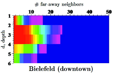
Figure 1: The cumulative distributions of far-away neighbors in the dual graph of Bielefeld downtown. The cumulative degree distribution are shown in the first row. The cumulative distributions of far-away neighbors are encoded in the second and forthcoming rows. Probability is ranked from zero (dark blue) to 1 (red).

For regular graphs, the number of far-away neighbors grows up exponentially fast with the distance. In Figs. 1, 2, we have displayed the cumulative distribution functions $P_{d}(n)$ quantifying the probabilities of that an average street is interconnected with at least $n$ other streets within a distance $d$ calculated for the dual graphs of two German organic cities - the downtown of Bielefeld in Westphalia and Rothenburg ob der Tauber in Bavaria. It is obvious that most of the streets in these towns can be reached in three navigation steps. The compactness of German medieval towns (see Figs. 1, 2) uncovers the historical functional background beyond their structure.

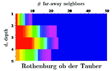
Figure 2: The cumulative distributions of far-away neighbors in the dual graphs of Rothenburg ob der Tauber, Bavaria. The cumulative degree distribution are shown in the first row. The cumulative distributions of far-away neighbors are encoded in the second and forthcoming rows. Probability is ranked from zero (dark blue) to 1 (red).

The term of a burgh has been in use since the $12^{\mathrm{th}}$ century, when David I of Scotland created the first Royal burghs. Early burghs were granted the power to trade, which allowed them to control trade until the $19^{\mathrm{th}}$ century, [27]. Their spatial structure was shaped by the public activities such as trade and exchange - ordered in such a way as to maximize the presence of people in central areas. In such an organic city, the majority of streets are just by a few syntactic steps away from each other, so that the entire city is compact that can be clearly seen from statistics of far away neighbors shown in Figs. 1-4.

It is interesting to mention that in the larger urban patterns such as the street grid in Manhattan and the canal network of Venice, most of the nodes of spatial networks can still be reached in less as three navigation steps (see. Figs. 3,4). However, there are also noticeable fractions of relatively isolated places.

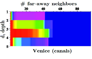
Figure 3: The cumulative distributions of far-away neighbors in the dual graph of Venetian canal network (96 canals). Probability is ranked from zero (dark blue) to 1 (red).

The structure of cumulative distributions shown in Figs. 3, 4 suggests that the correspondent graphs contain many cliques (complete subgraphs), together with subgraphs being ”almost” cliques. In complex network theory, this phenomenon is called the small world property. Small-world networks are characterized by a small diameter and a high clustering coefficient having connections between almost any two nodes within them. Hubs - nodes in the network serving as the common connections mediating the short path lengths between other edges are commonly associated with small-world networks, [28].

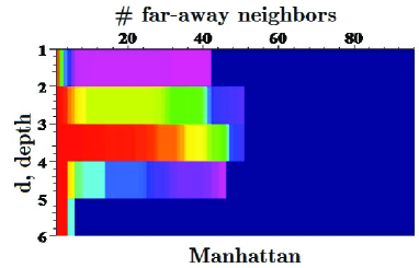
Figure 4: The cumulative distributions of far-away neighbors in the dual graph of the street grid in Manhattan. Probability is ranked from zero (dark blue) to 1 (red).

The tendency to shorten distances in urban space networks induced by the public processes is complemented in the ”small world” cities (like those represented in Fig. 3, 4) with the residential process which shapes relations between inhabitants and strangers preserving the original residential culture against unsanctioned invasion of privacy. While the majority of streets and canals characterized with an excellent accessibility promotes commercial activities and intensifies cultural exchanges, certain districts of such cities demonstrate the opposite tendency having residential areas relatively segregated from the rest of the city, [3].

The main technical problem of space syntax investigation is to rank out the open spaces in the city in accordance to their accessibility.

4 From random walks to Euclidean spaces

The idea of using the spectral properties of self-adjoint operators in order to extract information about graphs is standard in spectral graph theory [29] and in theory of random walks on graphs [14]-[16]. In the following calculations, in the transition operator (13) we take $\beta=1$ that allows to compare directly the forthcoming formulas with those known from the classical surveys on random walks defined on graphs, [14]-[16].

Among all measures which can be defined on the set of nodes $V$, there is one associated to the stationary distribution of random walks, $m=\sum_{i\in V}\pi_{i}\delta_{i}$, in which $\delta_{i}$ is the vector of the canonical basis that equals 1 at $i\in V$ and zero otherwise, with respect to which the transition operator ((13) with $\beta=1$) is self-adjoint in the Hilbert space $\mathcal{H}(V)$,

$$\widehat{T}\,=\,\frac{1}{2}\left(\pi^{1/2}T\pi^{-1/2}+\pi^{-1/2}T^{\top}\pi^{1/2}\right).$$ (18)

In the above equation, $T^{\top}$ is the adjoint operator, and $\pi$ is considered as the diagonal matrix $\mathrm{diag}\left(\pi_{1},\ldots,\pi_{N}\right)$. In particular, the elements of the symmetric transition operator defined on simple undirected graphs equal

$$\widehat{T}_{ij}\,=\,\frac{1}{\sqrt{k_{i}k_{j}}},\quad\mathrm{iff}\,\,i\sim j,$$ (19)

and zero otherwise.

The orthonormal ordered set of real eigenvectors $\psi_{i}$, $i=1\ldots N$, of the symmetric transition operator $\widehat{T}$ forms a basis in Hilbert space $\mathcal{H}(V)$. The components of the first eigenvector $\psi_{1}$ belonging to the largest eigenvalue $\mu_{1}=1$,

$$\psi_{1}\,\widehat{T}\,=\,\psi_{1},\quad\psi_{1,i}^{2}\,=\,\pi_{i},$$ (20)

describes the connectivity of nodes ($\pi_{i}\propto k_{i}$). The Euclidean norm of the orthogonal complement of $\psi_{1}$, $\sum_{s=2}^{N}\psi_{s,i}^{2}=1-\pi_{i}$, quantifies the probability that a random walker is not in $i$. The eigenvectors, $\left\{\,\psi_{s}\,\right\}_{s=2}^{N}$, belonging to the eigenvalues $1>\mu_{2}\geq\ldots\mu_{N}\geq-1$ describe the connectedness of the graph $G$. The exterior products of vectors calculated by means of determinants are used in Euclidean geometry to study areas, volumes, and their higher-dimensional analogs, [30]. Denote by $C_{m}$ the set of all subsets of $V$ containing precisely $1\leq m\leq N$ nodes. It is obvious that the size $\left|C_{m}\right|$ is given by the binomial coefficient,

$$\left|C_{m}\right|\,=\,\frac{N!}{m!(N-m)!}.$$

Let us note that the eigenvectors $\psi_{i}$, $i=1\ldots N$, induce basis systems for the spaces of all square summable $m$-point functions $f:\left\{i_{1},\ldots i_{m}\in V\right\}\to\mathbb{R}$. We consider the matrix of eigenvectors of the symmetric transition operator (20),

$$\Psi\,=\,\left(\begin{array}[]{ccc}\psi_{1,1}&\ldots&\psi_{1,N}\\ \vdots&\vdots&\vdots\\ \psi_{N,1}&\ldots&\psi_{N,N}\end{array}\right),$$ (21)

in which the rows $\left\{\psi_{k}\right\}_{k=1}^{N}$ are orthonormal, $\left(\psi_{i},\psi_{j}\right)=\delta_{ij}$. It is well known that $\det\Psi=\pm 1$ and numerically equal to the content of the parallelotope spanned by the unit eigenvectors $\left\{\psi_{k}\right\}_{k=1}^{N}$.

The nice property of minors $\Psi^{i_{1},\ldots i_{m}}_{s_{1},\ldots s_{m}}$ of order $m$ obtained by the deletion of $m$ rows $\left\{s_{l}\right\}$, $l=1,\ldots m$, and columns $\left\{i_{l}\right\}$, $l=1,\ldots m$, from $\det\Psi$ is that they are equal to their algebraic complements in $\Psi$, multiplied by $\pm 1$, [31]. Moreover, the complete set of minors of order $m$ forms an orthonormal system of $m-$point antisymmetric functions,

$$\sum_{i_{1},\ldots i_{m}}\Psi^{i_{1},\ldots i_{m}}_{s_{1},\ldots s_{m}}\Psi^{i_{1},\ldots i_{m}}_{s^{\prime}_{1},\ldots s^{\prime}_{m}}\,=\,\delta_{s_{1}s^{\prime}_{1}}\ldots\delta_{s_{m}s^{\prime}_{m}},$$ (22)

and can therefore be chosen as the basis in the Euclidean space $\mathbb{R}^{\left|C_{m}\right|}$, [31]. In the next section, we use the minors of order one to construct the embedding of undirected graphs into Euclidean space. In particular, we demonstrate that since any density $\sigma$ taken as an initial distribution of random walkers on an undirected graph converges to the unique stationary distribution $\pi$ as $t\to\infty$, this Euclidean space is $\mathbb{R}^{N-1}$.

The orthonormal systems of functions (22) are useful for decomposing the data when analyzing the traffic properties of transport networks. The data (say, of the real-time traffic flows and speed measurements) from $m$ different detectors taken at different time slices can be uniquely decomposed using the orthonormal system (22) into smaller, more manageable parts and then compared allowing therefore an effective classification of traffic speed patterns.

5 Euclidean embedding
of graphs by random walks

In the present section, we consider the orthogonal system of minors of order one, $\Psi_{s}^{i}$, which are numerically equal to the correspondent components of the eigenvectors $\psi_{s,i}$. In particular, it is clear that the minors $\left(\Psi_{1}^{i}\right)^{2}_{i}=\pi_{i}$ in accordance to (20). The minors of order one ($m=1$) are associated to the nodes of the graph and provide the basis for the Hilbert space $\mathcal{H}(V)$. We demonstrate that a simple undirected graph can be embedded into the $(N-1)$ Euclidean space, so that for any pair of nodes the distance and angle can be uniquely defined.

It is important to note that Markov’s symmetric transition operator $\widehat{T}$ defines a projection of any density $\sigma\in\mathcal{H}(V)$ on the eigenvector $\psi_{1}$ related to the stationary distribution $\pi$,

$$\sigma\,\widehat{T}\,=\,\psi_{1}+\sigma_{\bot}\,\widehat{T},\quad\sigma_{\bot}\,=\,\sigma-\psi_{1},$$ (23)

in which $\sigma_{\bot}$ is the vector belonging to the orthogonal complement of $\psi_{1}$. It follows from (16) that $\lim_{t\to\infty}\sigma_{\bot}\widehat{T}^{t}=0,$ so that the vector $\sigma_{\bot}$ characterizes the transient process induced by $\sigma$.

In space syntax, we are interested in a comparison between the different densities defined on the nodes of the graph. It is convenient to compare them in accordance to their proximity to the unique stationary distribution of random walks $\pi$ defined on the graph $G$. Since all components $\psi_{1,i}>0$, we can rescale the density $\sigma$ by dividing its components by the components of $\psi_{1}$,

$$\widetilde{\sigma_{i}}\,=\,\frac{\sigma_{i}}{\psi_{1,i}}\,=\,\frac{\sigma_{i}}{\sqrt{\pi_{i}}}.$$ (24)

It is clear that any two rescaled densities $\widetilde{\sigma},\widetilde{\rho}\,\in\,\mathcal{H}$ differ with respect to random walks only by their dynamical components orthogonal to $\psi_{1}$,

$$\left(\widetilde{\sigma}-\widetilde{\rho}\right)\,\widehat{T}^{t}\,=\,\left(\widetilde{\sigma}_{\bot}-\widetilde{\rho}_{\bot}\right)\,\widehat{T}^{t},$$

for all $t>0$.

Therefore, we can define the distance $\|\ldots\|_{T}$ based on random walks between any two densities by

$$\left\|\,\sigma-\rho\,\right\|^{2}_{T}\,=\,\sum_{t\,\geq\,0}\,\left\langle\,\widetilde{\sigma}_{\bot}-\widetilde{\rho}_{\bot}\,\left|\,\widehat{T}^{t}\,\right|\,\widetilde{\sigma}_{\bot}-\widetilde{\rho}_{\bot}\,\right\rangle.$$ (25)

or, using the spectral representation of $\widehat{T}$,

$$\begin{array}[]{l}\left\|\sigma-\rho\right\|^{2}_{T}\\ =\sum_{t\,\geq 0}\sum_{s=2}^{N}\,\mu^{t}_{s}\left\langle\widetilde{\sigma}^{\bot}-\widetilde{\rho}^{\bot}|\psi_{s}\right\rangle\!\left\langle\psi_{s}|\widetilde{\sigma}^{\bot}-\widetilde{\rho}^{\bot}\right\rangle\\ =\sum_{s=2}^{N}\,\frac{\left\langle\,\widetilde{\sigma}_{\bot}-\widetilde{\rho}_{\bot}\,|\,\psi_{s}\,\right\rangle\!\left\langle\,\psi_{s}\,|\,\widetilde{\sigma}_{\bot}-\widetilde{\rho}_{\bot}\,\right\rangle}{\,1\,-\,\mu_{s}\,},\end{array}$$ (26)

where we have used Dirac’s bra-ket notations especially convenient for working with inner products and rank-one operators in Hilbert space.

If we introduce a new inner product for densities $\sigma,\rho\in\mathcal{H}(V)$ by

$$\left(\,\sigma,\rho\,\right)_{T}\,=\,\sum_{s=2}^{N}\,\frac{\,\left\langle\,\widetilde{\sigma}_{\bot}\,|\,\psi_{s}\,\right\rangle\!\left\langle\,\psi_{s}\,|\,\widetilde{\rho}_{\bot}\right\rangle}{\,1\,-\,\mu_{s}\,},$$ (27)

then (26) is nothing else but

$$\left\|\,\sigma-\rho\,\right\|^{2}_{T}\,=\left\|\,\sigma\,\right\|^{2}_{T}+\left\|\,\rho\,\right\|^{2}_{T}-2\left(\,\sigma,\rho\,\right)_{T},$$ (28)

where

$$\left\|\,\sigma\,\right\|^{2}_{T}\,=\,\,\sum_{s=2}^{N}\,\frac{\left\langle\,\widetilde{\sigma}_{\bot}\,|\,\psi_{s}\,\right\rangle\!\left\langle\,\psi_{s}\,|\,\widetilde{\sigma}_{\bot}\,\right\rangle}{\,1\,-\,\mu_{s}\,}$$ (29)

is the square of the norm of $\sigma\,\in\,\mathcal{H}(V)$ with respect to random walks defined on the graph $G$.

We conclude the description of the $(N-1)$-dimensional Euclidean space structure of $G$ induced by random walks by mentioning that given two densities $\sigma,\rho\,\in\,\mathcal{H}(V),$ the angle between them can be introduced in the standard way,

$$\cos\,\angle\left(\rho,\sigma\right)=\frac{\,\left(\,\sigma,\rho\,\right)_{T}\,}{\left\|\,\sigma\,\right\|_{T}\,\left\|\,\rho\,\right\|_{T}}.$$ (30)

Random walks embed connected undirected graphs into the Euclidean space $\mathbb{R}^{N-1}$. This embedding can be used in order to compare the accessibility properties of individual nodes and to construct the optimal coarse-graining representations of the transport networks.

Indeed, the vector $\delta_{i}$ of the canonical basis is the particular case of density, which is zero for all nodes excepting for the node $i\in V$ where it equals 1. In accordance to (29), the density $\delta_{i}$ acquires the norm $\left\|\,\delta_{i}\,\right\|_{T}$ associated to random walks defined on $G$. In the theory of random walks [14], its square,

$$\left\|\,\delta_{i}\,\right\|_{T}^{2}\,=\,\frac{1}{\pi_{i}}\,\sum_{s=2}^{N}\,\frac{\,\psi^{2}_{s,i}\,}{\,1-\mu_{s}\,},$$ (31)

gets a clear probabilistic interpretation expressing the spectral formula of access time to the node $i\in V$, the expected number of steps required for a random walker to reach the node $i$ starting from an arbitrary node chosen randomly among all other nodes of the graph $G$ with respect to the stationary distribution of random walks $\pi$. The squared norm of the canonical vector $\left\|\,\delta_{i}\,\right\|_{T}^{2}$ can be used in order to characterize the access to the node $i$ from other nodes of the graph $G$. By the inequality between arithmetic and harmonic means, it is easy to prove [14] that

$$\left\|\,\delta_{i}\,\right\|_{T}^{2}\,\geq\,\frac{\left(1-\pi_{i}\right)^{2}}{\pi_{i}},$$ (32)

so that the nodes which are difficult to reach ($\pi_{i}\ll 1$) are also isolated from the rest of the graph.

The Euclidean distance between any two nodes of the graph $G$ is calculated as the distance (26) induced by random walks between two canonical vectors $\delta_{i}$ and $\delta_{j}$,

$$K_{i,j}\,=\,\left\|\,\delta_{i}-\delta_{j}\,\right\|^{2}_{T}\,=\,\sum_{s=2}^{N}\,\frac{1}{1-\mu_{s}}\left(\frac{\psi_{s,i}}{\sqrt{\pi_{i}}}-\frac{\psi_{s,j}}{\sqrt{\pi_{j}}}\right)^{2},$$ (33)

gives the spectral representation of commute time defined in the theory of random walks on undirected graphs as the expected number of steps required for a random walker starting at $i\,\in\,V$ to visit $j\,\in\,V$ and then to return back to $i$, [14].

The commute time which plays the role of the Euclidean distance between the nodes of the graph can be represented as a sum, $K_{i,j}=H_{i,j}+H_{j,i}$, in which

$$H_{i,j}\,=\,\left\|\,\delta_{i}\,\right\|^{2}_{T}-\left(\,\delta_{i},\delta_{j}\,\right)_{T}$$ (34)

is the first hitting time which plays probably the most important role in the quantitative theory of random walks [14]. It quantifies the expected number of steps before node $j$ is visited if starting from node $i$. The first hitting time $H_{i,j}$ satisfies the equation

$$H_{i,j}\,=\,1+\frac{1}{k_{i}}\sum_{l\sim i}H_{l,j}$$ (35)

with the intimal condition $H_{i,i}=0$. The equation (35) expresses the fact that the first step takes the random walker to a neighbor $l\sim i$ and then he has to reach $j$ from there.

It is important to mention that the cosine of an angle calculated in accordance to (30) has the structure of Pearson’s coefficient of linear correlations that reveals it’s natural statistical interpretation. The notion of angle between any two nodes of the graph arises naturally as soon as we become interested in the strength and direction of a linear relationship between two random variables, the flows of random walks moving through them. If the cosine of an angle (30) is 1 (zero angles), there is an increasing linear relationship between the flows of random walks through both nodes. Otherwise, if it is close to -1, there is a decreasing linear relationship. The correlation is 0 if the variables are linearly independent. It is important to mention that as usual the correlation between nodes does not necessary imply a direct causal relationship (an immediate connection) between them.

6 Petersen graph and Venetian Canals

In the present section, we construct and investigate the Euclidean embedding of two graphs. The first one we study is the Petersen graph with 10 nodes (see Fig. 5). Another example is the spatial network of 96 Venetian canals which serve the function of roads in the ancient city that stretches across 122 small islands (see Fig. 6). While identifying canals over the plurality of water routes on the city map of Venice, the canal-named approach has been used, in which two different arcs of the city canal network were assigned to the same identification number provided they have the same name.

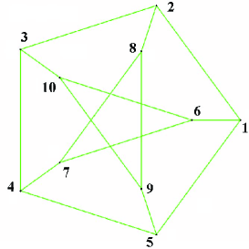
Figure 5: The Petersen graph.

The Petersen graph is a regular graph, $k_{i}=3$, $i=1,\ldots 10$, so that $\sum_{i}k_{i}=30$, and the stationary distribution of random walks is uniform, $\pi^{(\mathrm{Pet})}_{i}=0.1$. The spectrum of the random walk transition operator (18) defined on the Petersen graph contains the Perron eigenvalue $\mu_{1}=1$ which is simple, then the eigenvalue $\mu_{2}=1/3$ with multiplicity $5$, and $\mu_{3}=-2/3$ with multiplicity $4$. Therefore, there are just $3$ linearly independent eigenvectors, and two eigensubspaces for which the orthonormal basis vectors can be calculated, so that the resulting matrix of eigenvectors and basis vectors which we use in (31-33) always has full column dimension.

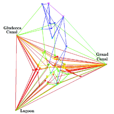
Figure 6: The dual graph representation of the spatial network of 96 Venetian canals

Random walks embed the Petersen graph into a $9$-dimensional Euclidean space, in which all nodes have equal norm (31), $\left\|i\right\|_{T}=3.14642654$ meaning that the expected number of steps a random walker starting from a node chosen randomly with probability $p=0.1$ reaches any node in the Petersen graph equals $9.9$.

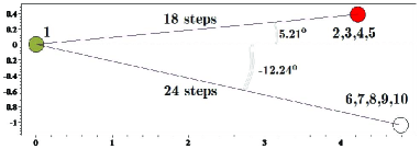
Figure 7: The Euclidean space embedding of the Petersen graph drawn with respect to the node $\#1$.

Indeed, the structure of $9$-dimensional vector space induced by random walks defined on the Petersen graph cannot be represented visually, however if we choose one node as a point of reference, we can draw its 2-dimensional projection by arranging other nodes at the distances calculated accordingly to (33) and under the angles (30) they are with respect to the chosen reference node (see Fig. 7).

It is expected that a random walker starting at the node $1$ visits any peripheral node ($2,3,4,5$) and then returns back in 18 random steps, while 24 random steps are expected in order to visit any internal node in the deep of the graph ($6,7,8,9,10$). It is also obvious that while the linear relationship between the random walks flows through the node $1$ and those through any peripheral node is positive, it is negative with respect to the flows passing through the internal nodes. Due to the symmetry of the Petersen graph, the figure displayed on Fig. 7 is essentially the same if we draw it with respect to any other periphery node ($2,3,4,5$). It is also important to note that it turns to be mirror-reflected if we draw it with respect to any internal node ($6,7,8,9,10$). Therefore, we can conclude that the Petersen graph contains two groups of nodes, at the periphery and in the depth, which appears to be as much as a quarter more isolated from one another than the nodes within each group (18 random steps vs. 24 random steps). It is clear that the $9-$dimensional embedding of the Petersen graph into Euclidean space is characterized by the highest degree of symmetry.

The dual graph of the spatial network of Venetian canals (Fig 6) is much more complicated than the Petersen graph. We construct it by mapping every canal into an individual node of the dual graph and connecting the pairs of nodes by arcs when these canals intersect. The resulting graph is far from being regular, so that the stationary distribution of random walks defined on it is not uniform. In [21], we have discussed that it is not evident if the degree distributions observed in compact urban patterns and in the Venetian canal network, in particular, follow a power law. The spectrum of the symmetric Markov transition operator (18) defined on that is presented in Fig. 8.

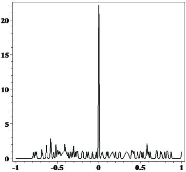
Figure 8: The spectrum of the Markov transition operator (19) defined on the spatial network of Venetian canals.

The transition matrix $\widehat{T}$ for the canal network in Venice is strongly defective. In particular, it contains the eigenvalue $\mu=0$ with multiplicity 22. This degeneracy indicates the presence of a complete bipartite subgraph in the spatial network of Venice shown in Fig. 6.

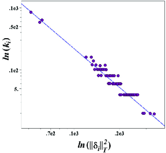
Figure 9: The scatter plot (in the log-log scale) of the connectivity vs. the value of access time to a node in the dual graph representation of 96 Venetian canals. Three data points characterized by the shortest access times represent the main water routes of Venice: the Lagoon of Venice, the Giudecca canal, and the Grand canal. Four data points of the worst accessibility are for the canal subnetwork of Venetian Ghetto. The slope of the regression line equals 2.07.

In urban spatial networks encoded by their dual graphs, the values of access time (31) vary strongly from one canal to another being very long for topologically isolated places. Three data points characterized by the shortest access times shown in Fig. 9 are associated to the Lagoon of Venice, the Giudecca canal, and the Grand canal - the most central water routes in the city canal network. Four data points characterized by the worst accessibility represent the canal subnetwork of Venetian Ghetto.

The values of access times observed in the dual graph of Venetian canals scale with the connectivity of canals: the slope of the regression line equals 2.07.

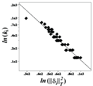
Figure 10: The scatter plot of the connectivity vs. the norm a node in the dual graph representation of 50 streets in the downtown of Bielefeld. The slope of the regression line equals 2.17.

A similar power law can be observed for the isolation patterns in other urban environments. For example, in Fig. 10, we have sketched the scatter plot of the connectivity vs. the norm a node in the dual graph representation of 50 streets in the downtown of Bielefeld. Professor Dr. Ludwig Streit works at the University of Bielefeld since 1972.

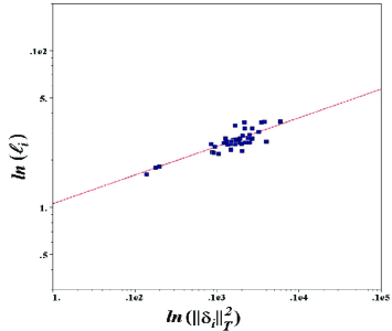
Figure 11: The scatter plot (in the log-log scale) of the mean shortest distance vs. the value of access time for the network of Venetian canals. The plot indicates a positive relation with the slope of regression line equals 0.18.

In the space syntax analysis, the mean shortest distance from a given node $i$ to any other node in the graph,

$$\ell_{i}\,=\,\frac{1}{N-1}\sum_{j\in V}d_{ij},$$ (36)

is used for characterizing the level of integration of the node in the city pattern, [22]. The relation between the mean shortest distance to a node $\ell_{i}$ and the value of access time to the same node $\left\|\delta_{i}\right\|^{2}_{T}$ is very complicated and strongly depends on the topology of the graph. In Fig. 11, we have shown the scatter plot (in the log-log scale) of the mean shortest distance vs. the value of access time for the network of Venetian canals. The plot Fig. 11 indicates a positive relation between $\ell_{i}$ and $\left\|\delta_{i}\right\|^{2}_{T}$ with the slope of the regression line equals 0.18.

The 2-dimensional projection of the Euclidean space of 96 Venetian canals set up by random walks drawn for the the Grand Canal of Venice (the point $(0,0)$) is shown in Fig. 12. Nodes of the dual graph representation of the canal network in Venice are shown by disks with radiuses taken equal to the degrees of the nodes. All distances between the chosen origin and other nodes of the graph (Fig. 6) have been calculated in accordance to (33) and (30) has been used in order to compute angles between nodes. Canals negatively correlated with the Grand Canal of Venice are set under negative angles (below the horizontal), and under positive angles (above the horizontal) if otherwise.

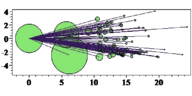
Figure 12: The 2-dimensional projection of the 95-dimensional Euclidean spaces associated to random walks defined on the city canal network built from the perspective of the Grand canal of Venice chosen as the origin. The labels of the horizontal axes display the expected number of random walk steps. The labels of the vertical axes show the degree of nodes (radiuses of the disks).

It is evident from Fig. 12 that disks of smaller radiuses demonstrate a clear tendency to be located far away from the origin being characterized by excessively long commute times with the reference node (the Grand canal of Venice), while the large disks which stand in Fig. 12 for the main water routes are settled in the closest proximity to the origin that intends an immediate access to them.

7 Discussion and Conclusion

From Euler’s time, urban design and townscape studies were the sources of inspiration for the network analysis and graph theory. It is common now that networks are the reality of urban renewals [32]. Flows of pedestrians and vehicles through a city are dependent on one another and that requests for organizing them in a network setting. Moreover, the networking is structurally contagious. In order to be able to master a network effectively, an authority should also constitute a network structure, probably as complicated as the one that it supervises. A complex network of city itineraries that we can experience in everyday life appears as the result of multiple complex interactions between various transport, social, and economical networks.

In the present paper, we have developed a self-consistent approach for exploring the structure of urban environments based on the use of Markov chains (random walks) defined on the dual graph of the city. The stochastic transition matrix of random walks gives a matrix representation for the group of automorphisms of the graph $G(V,E)$. The expected number of steps required to reach a node of the graph starting from a node chosen from the stationary distribution over $V$ given by (31) can be considered as a characteristic time scale $\mathcal{T}_{[i]}=\left\|\delta_{i}\right\|^{2}_{T}$ quantifying the accessibility of the node $i$ in the graph $G$ by random walks. The data of scatter plots displayed in Figs. 9,10 show that in the studied urban patterns $\mathcal{T}_{[i]}$ scales with the degree of vertex, so that $\mathcal{T}(k)\propto k^{-2-2\varepsilon}$, with some $\varepsilon>0$ ($\varepsilon=0.085$ for the downtown of Bielefeld and $\varepsilon=0.035$ for the canal network of Venice). We have also discussed in Sec. 2.1 that in the free flow regime of a queuing network preserving the proportion of time $\lambda_{i}$ spent in $i\in V$ constant (which then can be considered as the normalized length distance of the given street $i$), the expected first passage time to the node from a node random chosen among all nodes of the queuing network equals $\lambda_{i}^{-1}$. While equalizing these passage times, we obtain that in the free flow regime the proportion of time $\lambda$ spent by a moving agent in an open place of the given transport network scales with its connectivity as

$$\lambda(k)\,\propto\,k^{2+2\varepsilon},$$ (37)

where the value $\varepsilon>0$ is determined by the entire topology of the city.

It is well documented that isolation worsens an area’s economic prospects by reducing opportunities for commerce, and engenders a feeling of isolation for the inhabitants, both of which can fuel poverty and crime [3]. The method we have introduced in the present paper could easily be used to identify isolated neighborhoods in big cities with a complex web of roads, walkways and public transport systems spotting hidden areas of geographical isolation in the urban landscape. The method can be used to analyze complex transport networks of any type.

References

- [1] Famous Quotations/Stories of Winston Churchill at http://www.winstonchurchill.org.
- [2] B. Hillier, J. Hanson, The Social Logic of Space (1993, reprint, paperback edition ed.). Cambridge: Cambridge University Press (1984).
- [3] B. Hillier, The common language of space: a way of looking at the social, economic and environmental functioning of cities on a common basis, Bartlett School of Graduate Studies, London (2004).
- [4] B. Hillier, S.Iida, ”Network and psychological effects in urban movement”, in A.G. Cohn, D.M. Mark (eds) Proc. of Int. Conf. in Spatial Information Theory: COSIT 2005 published in Lecture Notes in Computer Science 3693, 475-490, Springer-Verlag, (2005).
- [5] N. Biggs, E. Lloyd, and R. Wilson, Graph Theory, 1736-1936. Oxford University Press (1986).
- [6] M. Chown, ”The Future Poverty Hiding In Cities”, The New Scientist: 3 November 2007 (# 2628), London.
- [7] B. Hughes, Random Walks and Random Environments, Vol. 1, Sec. 2.1 (Oxford, 1995).
- [8] B. Tadic, ”Exploring Complex Graphs by Random Walks”, in P. Garrido and J. Marro (Eds.), Modeling of complex systems: Seventh Granada Lectures, Granada, Spain, AIP Conference Proceedings, 661, pp. 24-26, Melville: American Institute of Physics, (2002).
- [9] Shi-Jie Yang, ”Exploring complex networks by walking on them”, Phys. Rev. E 71, 016107, URL: http://link.aps.org/abstract/PRE/v71/e016107; doi:10.1103/PhysRevE.71.016107 (2005).
- [10] Luciano da Fontoura Costa and Gonzalo Travieso, ”Exploring complex networks through random walks”, Phys. Rev. E 75, 016102; URL: http://link.aps.org/abstract/PRE/v75/e016102; doi:10.1103/PhysRevE.75.016102 (2007).
- [11] L. Breuer, D. Baum, An Introduction to Queueing Theory, Springer (2005).
- [12] S. Condamin, O Bénichou, V.Tejedor, R. Voituriez, J. Klaffer, First-passage times in complex scale-invariant media, Nature 450, 77 -79; doi:10.1038/nature06201.
- [13] D.J. Aldous, ”Lower Bounds for Covering Times for Reversible Markov Chains and Random Walks on Graphs”, J. Theor. Probab. 2 (1) (1989).
- [14] L. Lovász, ”Random Walks On Graphs: A Survey”, Bolyai Society Mathematical Studies 2: Combinatorics, Paul Erdös is Eighty, Keszthely (Hungary), p. 1-46 (1993).
- [15] L. Lovász, P. Winkler, Mixing of Random Walks and Other Diffusions on a Graph. Surveys in combinatorics, Stirling, pp. 119 154 (1995); London Math. Soc. Lecture Note Ser., vol. 218, Cambridge Univ. Press.
- [16] D.J. Aldous, J.A. Fill, Reversible Markov Chains and Random Walks on Graphs. A book in preparation, available at www.stat.berkeley.edu/aldous/book.html.
- [17] R.A. Horn, C.R. Johnson, Matrix Analysis, Cambridge University Press, 1990 (chapter 8).
- [18] W. G. Hansen, Journal of the American Institute of Planners 25, 73-76 (1959) .
- [19] A. G. Wilson, Entropy in Urban and Regional Modelling, Pion Press, London (1970).
- [20] M. Batty, A New Theory of Space Syntax, UCL Centre For Advanced Spatial Analysis Publications, CASA Working Paper 75 (2004).
- [21] Ph. Blanchard, D. Volchenkov, ”Random Walks along the Streets and Channels in Compact Cities: Spectral analysis, Dynamical Modularity, Information, and Statistical Mechanics”, Phys. Rev. E 75, 026104 (2007). URL:http://link.aps.org/abstract/PRE/v75/e026104.
- [22] B. Jiang, ”A space syntax approach to spatial cognition in urban environments”, Position paper for NSF-funded research workshop Cognitive Models of Dynamic Phenomena and Their Representations, October 29 - 31, 1998, University of Pittsburgh, Pittsburgh, PA (1998).
- [23] A. Cardillo, S. Scellato, V. Latora, and S. Porta, Phys. Rev. E 73, 066107 (2006).
- [24] S. Porta, P. Crucitti, and V. Latora, Physica A 369, 853 (2006)
- [25] S. Scellato, A. Gardillo, V. Latora, and S. Porta, Eur. Phys. J. B 50, 221 (2006).
- [26] P. Crucitti, V. Latora, and S. Porta, Chaos 16, 015113 (2006).
- [27] G.R. Stewart, Names on the Land. Boston: Houghton Mifflin Company (1967).
- [28] M. Buchanan, Nexus: Small Worlds and the Groundbreaking Theory of Networks. Norton, W. W. and Co., Inc. ISBN 0-393-32442-7 (2003).
- [29] F. Chung, Lecture notes on spectral graph theory, AMS Publications Providence (1997).
- [30] S. MacLane, G. Birkhoff, Algebra, AMS Chelsea (1999).
- [31] T. Muir, Treatise on the Theory of Determinants. Dover, New York, 1960 (revised and enlarged by W. H. Metzler).
- [32] M. Haffner, M. Elsinga, Urban renewal performance in complex networks Case studies in Amsterdam North and Rotterdam South, W16 Institutional and Organizational Change in Social Housing Organization in Europe, Int. Conference on Sustainable Urban Areas, Rotterdam (2007).