1]School of Mathematics and Statistics, University of St. Andrews, St. Andrews, KY16 9SS, United Kingdom 2]Max-Planck-Institut für Aeronomie, Max-Planck-Strasse 2, 37191 Katlenburg-Lindau, Germany
Wiegelmann \proofsT. Wiegelmann \offsetsT. Wiegelmann
Nonlinear Processes in Geophysics, Volume 10, Issue 4/5, 2003, pp.313-322
25 \pubnum2
Computing nonlinear force free coronal magnetic fields.
Zusammenfassung
Knowledge of the structure of the coronal magnetic field is important for our understanding of many solar activity phenomena, e.g. flares and CMEs. However, the direct measurement of coronal magnetic fields is not possible with present methods, and therefore the coronal field has to be extrapolated from photospheric measurements. Due to the low plasma beta the coronal magnetic field can usually be assumed to be approximately force free, with electric currents flowing along the magnetic field lines. There are both observational and theoretical reasons which suggest that at least prior to an eruption the coronal magnetic field is in a nonlinear force free state. Unfortunately the computation of nonlinear force free fields is way more difficult than potential or linear force free fields and analytic solutions are not generally available. We discuss several methods which have been proposed to compute nonlinear force free fields and focus particularly on an optimization method which has been suggested recently. We compare the numerical performance of a newly developed numerical code based on the optimization method with the performance of another code based on an MHD relaxation method if both codes are applied to the reconstruction of a semi-analytic nonlinear force-free solution. The optimization method has also been tested for cases where we add random noise to the perfect boundary conditions of the analytic solution, in this way mimicking the more realistic case where the boundary conditions are given by vector magnetogram data. We find that the convergence properties of the optimization method are affected by adding noise to the boundary data and we discuss possibilities to overcome this difficulty.
1 Introduction
The magnetic field is the most important quantity for understanding the plasma structure of the solar corona and the activity phenomena it shows. Unfortunately a systematic direct measurement of the coronal magnetic field is not feasible with the observational methods presently available. Therefore the extrapolation of the magnetic field into the corona from measurements of the magnetic field at the photospheric level is extremely important.
It is generally assumed that the magnetic pressure in the corona is much higher than the plasma pressure (small plasma ) and that therefore the magnetic field is nearly force-free (for a critical view of this assumption see Gary, 2001). The extrapolation methods based on this assumption include potential field extrapolation (e.g., Schmidt, 1964; Semel, 1967), linear force-free field extrapolation (e.g., Chiu and Hilton, 1977; Seehafer, 1978, 1982; Semel, 1988) and nonlinear force-free field extrapolation (e.g., Amari et al., 1997). Methods for non-force-free field extrapolation have also been developed (Petrie and Neukirch, 2000) but are not used routinely.
Whereas potential and linear force-free fields can be used as a first step to model the general structure of magnetic fields in the solar corona, the use of non-linear force free fields is essential to understand eruptive phenomena as there are both observational and theoretical reasons which suggest that the pre-eruptive magnetic fields are non-linear force-free fields (see below). The calculation of nonlinear force free fields is complicated by the intrinsic nonlinearity of the underlying mathematical problem. Another problem which becomes especially important when nonlinear force free field are used for magnetic field extrapolation is the correct formulation of the problem with respect to boundary values. The available magnetograph observation provide either the line-of-sight magnetic field (), which is sufficient for potential and linear force free fields, or all three components of the photospheric magnetic field. Only the latter information is sufficient to determine non-linear force free fields completely. There are, however, tremendous difficulties to be overcome both in extracting the necessary information about the magnetic field components on the boundary from the data in an unambiguous way and in the use of this information in the computation of the corresponding magnetic field. Even though a lot of research has been devoted to these problems in the past so far none of the proposed methods has been found to be outstanding in combining simplicity, usability and robustness.
The purpose of the present contribution is to assess some of the methods presently available for calculating non-linear force-free fields, with a view to implementing them into a general extrapolation code which also takes stereoscopic information into account in the extrapolation process. A first version of such a method based on linear force free extrapolation has recently been proposed (Wiegelmann and Neukirch, 2002). As stated in Wiegelmann and Neukirch (2002) and bearing in mind the remarks above, it is would be very desirable to generalize the extrapolation method to nonlinear force free fields.
As a first step in this direction we investigate the robustness of the optimization method recently proposed by Wheatland et al. (2000), and compare its performance with another method based on MHD relaxation. The paper is organized as follows. In Sect. 2 we discuss the basic equations and background theory. Section 3 describes various methods which have been proposed for nonlinear force free field extrapolation. Out of these we focus on the optimisation method and, for the case of analytically given boundary data, on the MHD relaxation method. These methods are tested using an analytical solution in Sect. 4. The optimisation method is also subjected to tests with more general boundary conditions where we add noise to the given analytical boundary data. The paper closes with the conclusions in Sect. 5.
2 Basic equations: Force-Free Equilibria
For force free fields the equations to solve are
| (1) | |||||
| (2) | |||||
| (3) |
Equation (1) implies that for force free fields the current density and the magnetic field are parallel, i.e.
| (4) |
Here is a function of space. This function has to satisfy the equation
| (5) |
which is obtained by taking the divergence of Eq. (4) and making use of Eqs. (2) and (3). Substituting Eq. (4) into Eq. (2) we get a second equation which determines :
| (6) |
Equation (5) implies that is constant along magnetic field lines, but that it can vary across the magnetic field. Obviously, Eq. (5) is solved by implying that by Eq. (4). In this case we obtain potential fields. Another obvious possibility is constant, but nonzero. This is the case of linear (or constant-) force free fields. Standard methods for calculating potential and linear force free field are available (see e.g. Gary, 1989) and they can at least give a rough impression of the coronal magnetic field structure.
There are, however, both observational and theoretical arguments that at least the magnetic field prior to eruptive processes in the corona is not a linear force free (or potential) field. If the normal component or the line-of-sight component of the magnetic field on the boundary is given the corresponding potential field is uniquely determined and is actually the magnetic field with the lowest magnetic energy for this boundary condition. Since magnetic energy is needed to drive an eruptive process pre-eruptive coronal magnetic fields cannot be expected to be in a potential state. This is also corroborated by observations (e.g. Hagyard, 1990; Hagyard et al., 1990; Falconer et al., 2002). Similar observations also indicate that it will usually be difficult to match the boundary magnetic field with a linear force-free field. Also, from a more general point of view it seems highly unlikely that the complex pre-eruption coronal magnetic field which is slowly but constantly stressed by changing boundary conditions will have the current density distribution of a linear force-free field, i.e. a constant . A (strongly) localized current density in the erupting configuration seems to be a lot more natural. Another argument which is sometimes put forward to rule out linear force-free magnetic fields for models of pre-eruptive states is that linear force free fields minimize the magnetic energy under the assumption of global helicity conservation (e.g., Taylor, 1974), and therefore if helicity conservation could be assumed to hold for a coronal eruption, a linear force-free field would not be able to provide the energy for the eruption. Even though it has been proposed to apply variants of Taylor’s hypothesis to the state of the coronal magnetic field on larger scales (e.g., Heyvaerts and Priest, 1984), it generally does not seem to apply for models of eruptive processes (e.g., Amari and Luciani, 2000). Furthermore, there is the possibility of helicity transport into and out of the region of interest and for these reasons, we do not want to put too much emphasis on this argument.
However, we believe that the other arguments are strong enough to assume that generally one has to take into account that for the force free magnetic fields of pre-eruptive states the value of changes from field line to field line. This automatically leads us to consider nonlinear force free fields.
3 Extrapolation Methods
The problem we discuss in this section is to compute nonlinear force free magnetic fields in Cartesian coordinates if given all three components of the magnetic field on the boundary, i.e. the photosphere. Various methods have been proposed (see e.g. Amari et al., 1997; Démoulin et al., 1997; McClymont et al., 1997; Semel, 1998; Amari et al., 2000; Yan and Sakurai, 2000) of which we will discuss three. For the first method we assume that the magnetic field is given on the lower boundary (photosphere), whereas for the second and third method we assume that is prescribed on the surfaces of a volume .
3.1 Direct Extrapolation
Direct extrapolation (Wu et al., 1990) is a conceptually simple method, in which the Eqs. (6) and (5) are reformulated in such way that they can be used to extrapolate the photospheric boundary conditions given by a vector magnetogram into the solar corona.
If we suppose that the boundary condition on the lower boundary is given by then we can calculate the -component of the current density at by using Eq. (2)
| (7) |
Knowing the -component of the photospheric magnetic field (), we can use Eqs. (7) and (4) to determine :
| (8) |
We remark that special care has to be taken at photospheric polarity inversion lines, i.e. lines along which (see e.g., Cuperman et al., 1991). Equation (8) allows us to calculate the and -component of the current density using Eq. (4)
| (9) | |||||
| (10) |
We now use Eq. (3) and the and -component of Eq. (2) to obtain expressions for the -derivatives of all three magnetic field components in the form
| (11) | |||||
| (12) | |||||
| (13) |
The idea is to integrate this set of equations (numerically) in the direction of increasing , basically repeating the previous steps at each height.
Unfortunately it can be shown that the formulation of the force free equations in this way is unstable because it is an ill-posed problem (e.g., Cuperman et al., 1990; Amari et al., 1997). In particular one finds that exponential growth of the magnetic field with increasing height is a typical behaviour. The reason for this is that the method transports information only from the photosphere upwards. Other boundary conditions. e.g. at an upper boundary, either at a finite height or at infinity cannot be taken into account. Attempts have been made to regularize the method (e.g., Cuperman et al., 1991; Démoulin et al., 1992), but cannot be considered as fully successful.
3.2 MHD-Relaxation
Another possibility to calculate nonlinear force free fields is by the method of MHD relaxation (e.g., Chodura and Schlüter, 1981). The idea is to start with a suitable magnetic field which is not in equilibrium and to relax it into a force free state. This is done by using the MHD equations in the following form :
| (14) | |||||
| (15) | |||||
| (16) | |||||
| (17) |
The equation of motion (14) has been modified in such a way that it ensures that the (artificial) velocity field is reduced. Equation (15) ensures that the magnetic connectivity remains unchanged during the relaxation. The relaxation coefficient can be chosen in such way that it accelerates the approach to the equilibrium state. We use
| (18) |
with constant. Choosing the relaxation coefficient proportional to speeds up the relaxation process in regions of weak magnetic field (see Roumeliotis, 1996). Combining Eqs. (14), (15), (16) and (18) we get an equation for the evolution of the magnetic field during the relaxation process :
| (19) |
This equation is then solved numerically starting with a given initial condition for . Equation (19) ensures that Eq. (17) is satisfied during the relaxation if the initial magnetic field satisfies it.
The difficulty with the relaxation method in the present form is that it cannot be guaranteed that for the boundary conditions we impose and for a given initial magnetic field (i.e. given connectivity), a smooth force-free equilibrium exists to which the system can relax. If such a smooth equilibrium does not exist the formation of current sheets is to be expected which will lead to numerical difficulties. Therefore, care has to be taken when choosing an initial magnetic field. This clearly limits the applicability of the relaxation method, and further work will be needed to overcome this obstacle. We therefore only apply the relaxation method for comparison with the optimization method to cases where we know the boundary conditions to be compatible.
One can show, however, that the relaxation method converges under less restrictive boundary conditions. By multiplying Eq. (16) by , integrating over the complete computational volume and using Eq. (15), we find that
| (20) |
where
| (21) |
Under line-tying boundary conditions we have on the boundary, and only the volume integral survives. Using Eq. (14) and the fact that one can show that in this case
| (22) |
and an equilibrium is achieved if and only if the magnetic field is force free.
We emphasize that these boundary conditions are usually not compatible with prescribing all three magnetic field components on the boundaries, but only the normal component. Therefore, in the following we discuss the relaxation method only for test cases in which we know that the boundary conditions are compatible. This is done for comparison with the other method we discuss now, the optimization method.
3.3 Optimization
Recently Wheatland et al. (2000) have proposed an optimization method which refines a proposal by Roumeliotis (1996). In this method the functional
| (23) |
is minimized. Obviously, is bounded from below by . This bound is attained if the magnetic field satisfies the force free equations
| (24) | |||||
| (25) |
The variation of with respect to an iteration parameter leads to (see Wheatland et al. (2000) for details)
| (26) |
where
| (27) | |||||
| (28) | |||||
| (29) |
The surface term in (26) vanishes for 111This condition makes it necessary that all three components of the magnetic field have to be prescribed on the six boundaries of the computational box. In section 4.2.3 we discuss how the surface integral in (26) can be used to update the lateral and top boundary conditions during the optimization process. Under this condition only the bottom boundary is prescribed time independently with the help of photospheric vector magnetograms. on the boundary and decreases for
| (30) |
This leads to an iteration procedure for the magnetic field which is based on the equation
| (31) | |||||
Here is a constant which can be chosen to speed up the convergence of the iteration process. Equation (19) and the leading terms of Eq. (31) are identical, but Eq. (31) contains additional terms.
For this method the vector field is not necessarily solenoidal during the computation, but will be divergence-free if the optimal state with is reached. A disadvantage of the method is that it cannot be guaranteed that this optimal state is indeed reached for a given initial field and boundary conditions. If this is not the case then the resulting will either be not force free or not solenoidal or both.
4 Tests
We encoded the MHD-relaxation method and the optimization method in one program. The code is written in C and uses 4th order finite differences on an equal spaced grid. The time iteration is computed with the method of steepest gradient (see e.g. text books like Geiger and Kanzow, 1999). The program is parallelized with OpenMP.
4.1 The semi-analytical test field
To test the reconstruction methods, we try to reconstruct a semi-analytic nonlinear force free solution found by Low and Lou (1990). Wheatland et al. (2000) have used similar tests. The main difference between their paper and ours is in the diagnostic quantities used and in the comparison with i) the relaxation method and ii) the noisy boundary data (which we think is more representative of a realistic situation). Low and Lou (1990) solved the Grad-Shafranov equation for axis-symmetric force free fields in spherical coordinates , , . For axis-symmetry the magnetic field can be written in the form
| (32) |
where is the flux function, and represents the -component of , depending only on . The flux function satisfies the Grad-Shafranov equation
| (33) |
where . Among others, Low and Lou (1990) derive solutions for
| (34) |
by looking for separable solutions of the form
| (35) |
The solutions are axis-symmetric in spherical coordinates with a point source at the origin, but if used for testing force free codes in Cartesian geometry the symmetry is no longer obvious after a translation which places the point source outside the computational domain and a rotation of the symmetry axis with respect to the Cartesian coordinate axis.
4.2 Test runs
For the test we have first calculated on the photospheric boundary for the appropriate Low and Lou solution. Using this as a boundary condition we calculate the potential field corresponding to this boundary conditions inside our computational box. The potential field is computed with help of a method developed by Seehafer (1978). This method gives the components of the magnetic field in terms of a Fourier series. The observed magnetogram (or here the extracted magnetogram from the Low and Lou solution) covers a rectangular region extending from to in and to in is artificially extended onto a rectangular region covering to and to by taking an antisymmetric mirror image of the original magnetogram in the extended region, i.e. and . We use a Fast Fourier Transformation (FFT) scheme (see Alissandrakis (1981)) to determine the coefficients of the Fourier series. For more details regarding this method see Seehafer (1978, 1982).
The potential field is used as starting field inside the computational box but the Low and Lou field is imposed on the boundaries. We then use either the MHD relaxation or the optimization method to calculate the correct force free equilibrium field. During the computations we calculate the quantities (for both relaxation and the optimization method), the absolute value of the Lorentz force (averaged over the numerical grid), the value of (averaged over the numerical grid), and the difference between the numerical magnetic field and the known analytical solution (averaged over the numerical grid) at each time step. In section 4.2.1 and 4.2.2 all components of the magnetic field are fixed on all six boundaries. In section 4.2.3 only the bottom boundary condition is prescribed time-independent and the lateral and top boundaries are updated during the iteration. The details are described in 4.2.3.
*
 \figbox*
 \figbox*
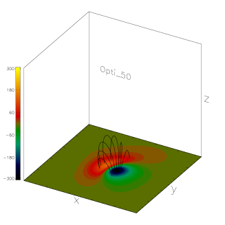

4.2.1 Standard tests
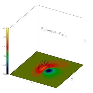
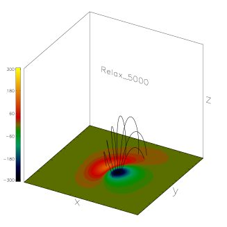
In Fig. 1 we show three-dimensional plots of selected magnetic field lines for the Low and Lou solution, the potential field calculated by taking the Low and Lou on the lower boundary, the field of the MHD relaxation method after , and relaxation time steps, and the same plots for the optimization method. In these runs we used a grid size of . The colour coding of the bottom boundary indicates the distribution on that boundary.
It can bee seen that the potential field which is used as starting field of the computations for both methods is clearly different from the Low and Lou test field. The state of the system after steps still shows some resemblance to the initial potential field for both methods but the field lines have started to evolve away from the potential field. One can also see small differences between the two methods. After steps no obvious differences between the magnetic field reached with either method and the Low and Lou field can be seen.

To quantify this statement we show in Fig. 2 a comparison of the evolution of the four diagnostic quantities for the two methods during the computation. For both methods all four diagnostic quantities decrease during the computation but after steps the optimization method shows significant smaller values for the quantities , and the comparison with the analytic solution. Therefore we can state that in this case the optimization method seems to be slightly more efficient than the MHD relaxation method.
| Step | Relative Error | |||
| discret. error | Reference | |||
| Start | 0 | |||
| Relaxation | 50 | |||
| 500 | ||||
| 5,000 | ||||
| Optimization | 50 | |||
| 500 | ||||
| 5,000 | ||||
| 1% noise | 5,000 | |||
| 10% noise | 5,000 | |||
| 20% noise | 5,000 | |||
| Pot-boundary | 500 | |||
| Pot-boundary | 5,000 | |||
| discret. error | Reference | |||
| Start | 0 | |||
| Optimization | 50 | |||
| 500 | ||||
| 5,000 | ||||
| 25,000 | ||||
| 10% noise | 25,000 | |||
| Pot-boundary | 1,000 | |||
| Pot-boundary | 10,000 |
This is corroborated by a look a Table 1 in which we summarize the main results of the various test runs we have made. The first row shows the discretisation errors for and the Lorentz force if the known solution is discretised on a -grid and used to calculate the values of this quantities. The second row contains the values of , the Lorentz force and the relative error after the interior grid points have been replaced by the potential field calculated from the photospheric of the Low and Lou solution. The relatively large values of the three diagnostic quantities show the deviation from the equilibrium.
The next two rows show how the three diagnostic quantities evolve during the MHD relaxation method for the -grid. One can see that after steps the value of has dropped by almost three orders of magnitude, but is still one order of magnitude above the value calculated with the discretised exact solution. The Lorentz force has dropped to the level of the dicretisation error, and the relative error has dropped more than two orders of magnitude.
We are giving the same quantities for the optimization method in the following three rows. It can be seen that especially the values of are always way below the corresponding values of the MHD relaxation method. This is not surprising as the optimization method relies on the minimization of the functional . The final value of is actually below the discretisation error. It can also be seen that the relative error after iterations is more than one order of magnitude smaller than the corresponding value of the MHD relaxation method.
We have made a step towards checking numerical convergence for the optimization method by repeating the calculation on a grid with doubled resolution (). The results are shown in the lower part of Table 1. The first thing to notice is that the discretisation error is almost an order of magnitude smaller than for the previous grid. For this grid iteration steps have been carried out, and after that the values of and the Lorentz force have reached the level of the discretisation error. The relative error is more than two orders of magnitude smaller than for the coarser grid.
4.2.2 Effect of adding noise
The previous calculations have been carried out under the assumption that the magnetic field on the boundary of the computational box is known exactly. Such an idealized situation will not be found when real data are used. Vector magnetograms will have finite resolution and suffer from observational uncertainties making the reconstruction potentially more difficult. Especially the optimization method has been proposed in view of coping with these difficulties (Wheatland et al., 2000).
*
To investigate how the optimization method works if the boundary conditions are not given by the exact analytical field, but to keep control over the amount of uncertainty, we have carried out test runs with the optimization method adding random noise with to the boundary conditions. We add the noise by multiplying the exact boundary conditions with a number where is a random number in the range and is the noise level.
To study the effect of the noise we have done runs with different amplitudes of noise on the grid. The evolution of and the Lorentz force with the numbers of iteration for various noise levels are shown in Fig. 3. It can clearly be seen that the method converges less and less well with increasing noise. For noise levels of 10 % and 20 %, the corresponding values after steps for the grid are given in Table 1. We have also carried out a run on the grid with a noise level of 10 %. For this run the values of the diagnostic quantities after steps are still higher than the values of the corresponding quantities on the coarser grid after steps. We have to conclude that even a 10 % uncertainty in the boundary conditions could affect the convergence of the optimization method quite badly. The main problem is that with noise and fixed boundary conditions on all six boundaries the boundary condition are over-imposed and will no longer be compatible. We discuss how this problem can be solved in the next section.
4.2.3 The problem of the lateral and top boundary conditions
Until now the runs have been carried out under the assumption that the magnetic field boundary conditions are well known on all six boundaries of the box. Unfortunately real vectormagnetograms only provide information regarding the photospheric magnetic field. The top and side boundary conditions are unknown and have to be fixed somehow. Here we want to investigate the influence of the choice of these boundary conditions. An additional problem occurs by fixing the vector magnetic field on all six boundaries (as done in the previous sections) because one overimposes the boundary conditions. For the test cases in the previous sections the boundary conditions have been extracted from an analytic solution and consequently the boundaries are automatically compatible (this implies that there are no problems with over-imposed boundary conditions). Section 4.2.2 showed that this compatibility might get lost if the boundaries contain noise. To overcome this difficulty and to take into account that measured data are only available for the bottom boundary we describe how the strict condition on all boundaries can be avoided within the optimization procedure. First we have to impose the boundary conditions as a well posed problem. A popular well posed boundary condition for non linear force free fields is to impose the normal component of the magnetic field and the normal component of the current density in regions for a positive (or negative) . (see Aly, 1989, regarding the compatibility of photospheric vector magnetograph data). These conditions have been derived under the very strict constraint of a flux balanced magnetogram where all magnetic flux is closed. This implies that each magnetic field line starting at one point on the photosphere also has to end on the photosphere (in a region of opposite magnetic flux, but with the same value of ). Such strictly isolated active regions seem to be a too restrictive constraint for real vector magnetograms. Real vectormagnetograms provide all three components of the magnetic field for either sign of and thus also on the complete bottom boundary. It seems reasonable to impose these observed data on the bottom boundary. The price we have to pay is that field lines starting on the photosphere might pass the lateral and top boundary. 222If the flux is not balanced in the region, it implies that part of the flux distribution is missing from the limited-size of the magnetogram or that the calibration of the magnetograph is bad. In both cases, any magnetic extrapolation method will only derive an approximate field. Unfortunately the size of observed vectormagnetograms is limited and a real magnetogram will usually not be exactly flux balanced. Field lines passing the boundary of the computational box can be either open field lines or close on the photosphere outside the observed magnetogram. Consequently we need to update the lateral and top boundary during the iteration.
As a first step towards consistent boundary conditions for the optimization method, we choose a potential field on the lateral and top boundaries. Firstly, a potential field can be easily computed just from the measured normal component of the photospheric magnetic field and secondly, it can be assumed that the solar magnetic field is reasonably well approximated by a potential field outside active regions. Here we compute the potential field on the boundary as a global potential field computed from the distribution at alone. Table 1 shows that the value of for the grid drops to a slightly lower value than for the corresponding run with noise, while the remaining forces are a factor of three lower. The relative error compared with the exact solution is quite high here, which is no wonder because the magnetic field is forced to stay potential close to the side and top boundaries. One might notice that the error in the forces is a factor of larger than the discretisation error, while is more than two orders of magnitude larger than the discretisation error. The reason is that an inconsistency occurs at the edges of the box between the photospheric boundary and the side boundaries. The Low and Lou solution is not potential on the photosphere close to the side boundaries, but the chosen side boundary conditions are potential.
To overcome this difficulty we cannot fix the lateral and top boundaries during the iteration, but have to relax also these boundaries. As the iteration equation (30) has been derived under the condition on all boundaries we have to extend the optimization approach. If we allow on some boundaries the surface term in equation (26) does not necessarily vanish. It is straightforward to extend the iteration by
| (36) |
on the open boundaries. Equation (36) changes the boundary values in such way that decreases. In the following we choose the lateral and top boundaries as open (they are initialized with a potential field) and apply Eq. (36) here. The bottom boundary remains time independent during the iteration. Let us remark that one might as well use the above described photospheric boundary condition for isolated active regions ( fixed on the photosphere only in regions of positive ). To do so one has to apply Eq. (36) also for the transversal magnetic field on the photosphere in regions with negative .
If we do not keep the lateral and top boundary conditions fixed, but allow them to relax with help of Eq. (36), L drops to which is only one order of magnitude above the discretisation error. The corresponding value of the total force decreases slightly () compared to fixed boundary conditions. For observed vectormagnetograms it might be useful to choose a sufficiently large area around an active region, i.e. with the side boundaries relatively far away from the non-potential active region, so that the magnetic field can be assumed to be approximately potential close to the side boundaries. We remark that it might be hard to find corresponding vector magnetograms as these instruments (e.g. IVM in Hawaii) do not observe the complete solar disk, but only restricted areas. We have also carried out a run on the grid with potential field boundary conditions. For this run a stationary state is reached after steps, and the forces are less than one order of magnitude higher than the discretisation error, while is nearly three orders of magnitude above the discretisation error. Please note that the absolute error in the has the same order of magnitude here as for the corresponding run. If we allow relaxation on the side and top boundaries, L drops to and is slightly higher than for fixed side boundary conditions. We conclude that the uncertainty of the side and top boundary conditions affects the convergence of the optimization method. Its influence can be reduced significantly if we allow for a relaxation of these boundaries and only fix the photospheric boundary conditions, but further improvements would still be welcome.
5 Conclusions
In the present paper we have presented an assessment of the properties of an optimization method which has recently been proposed for the calculation of nonlinear force-free fields from given boundary data (Wheatland et al., 2000). One part of the assessment was a comparison the performance of the optimization method with the performance of an MHD relaxation method. For both methods new parallelized codes have been developed. Both methods have been applied to finding a known semi-analytic solution (Low and Lou, 1990) from a given non-equilibrium initial condition. Both methods converge to the exact solution, but the optimization method has higher accuracy. The MHD relaxation method is only applied to this case since in its present numerical implementation, the boundary conditions could give rise to inconsistencies.
To simulate a more realistic situation which is closer to working with observational data from vector magnetograms we added noise to the boundary conditions. We have only applied the optimization method to this type of problem and found that already a relatively small noise level of 10 % can affect the convergence of the method quite considerably. More work is needed to see how this difficulty can be overcome. We also intend to generalize the relaxation method in such way that is able of coping with more realistic boundary data.
The ultimate aim for the future is to apply these methods to data from vector magnetograms. Unfortunately vector magnetograms are less accurate than line-of-sight magnetograms (e.g. from MDI on SOHO). Therefore, in the light of our results in the cases where noise was added to the boundary conditions it will be interesting to see whether and how quickly the methods converge. We also plan to use stereoscopic information as a further constraint in the reconstruction process. This will become especially important for the analysis of data from the STEREO mission. A method which is based on linear force free fields has recently been proposed by Wiegelmann and Neukirch (2002), but linear force free fields seem to be too restrictive to describe coronal phenomena appropriately. Therefore, the natural next step will be the use of nonlinear force free fields in such a code.
Acknowledgements.
The authors thank Bernd Inhester and Hardi Peter for useful discussions. TW acknowledges support by the European Communitys Human Potential Programme through a Marie-Curie-Fellowship. TN thanks PPARC for support by an Advanced Fellowship. The computations have been carried out on the PPARC funded MHD Cluster in St. Andrews. We thank Norbert Seehafer and an unknown referee fore useful comments.References
- Alissandrakis (1981) Alissandrakis, C.E.: On the computation of a constant- force-free magnetic field, Astron. Astrophys., 100, 197-200, 1981.
- Aly (1989) Aly, J. J: On the reconstruction of the nonlinear force-free coronal magnetic field from boundary data, Solar Phys., 120, 19-48, 1989.
- Amari and Luciani (2000) Amari, T. and Luciani, J. F.: Helicity redistribution during relaxation of astrophysical plasmas, Phys. Rev. Lett., 84, 1196-1199, 2000.
- Amari et al. (1997) Amari, T., Aly, J. J., Luciani, J. F., Boulmezaoud, T. Z., and Mikic, Z.: Reconstructing the solar coronal magnetic field as a force-free magnetic field, Solar Phys., 174, 129-149, 1997.
- Amari et al. (2000) Amari, T., Boulmezaoud, T. Z., and Mikic, Z.: An iterative method for the reconstruction of the solar magnetic field. I. Method for regular solutions, Astron. Astrophys., 350, 1051-1059, 2000.
- Chiu and Hilton (1977) Chiu, Y. T. and Hilton, H. H.: Exact Green’s function method of solar force-free magnetic-field computations with constant . I. Theory and basic test cases, Astrophys. J., 212, 873-885, 1977.
- Chodura and Schlüter (1981) Chodura, R., and Schlüter, A.: A 3-D code for MHD equilibrium and stability, J. Comp. Phys., 41, 68-88, 1981.
- Cuperman et al. (1990) Cuperman, S., Ofman, L., and Semel, M.: Determination of force-free magnetic fields above the photosphere using three-component boundary conditions: moderately non-linear case, Astron. Astrophys., 230, 193-199, 1990.
- Cuperman et al. (1991) Cuperman, S., Démoulin, P., and Semel, M.: Removal of singularities in the Cauchy problem for the extrapolation of solar force-free magnetic fields, Astron. Astrophys., 245, 285-288, 1991.
- Démoulin et al. (1992) Démoulin, P., Cuperman, S., and Semel, M.: Determination of force-free magnetic fields above the photosphere using three-component boundary conditions. II. Analysis and minimization of scale-related growing modes and of computational induced singularities, Astron. Astrophys., 263, 351-360, 1992
- Démoulin et al. (1997) Démoulin, P., Hénoux, J. C., Mandrini, C. H., and Priest, E. R.: Can we extrapolate a magnetic field when its topology is complex ?, Solar Phys., 174, 73-89, 1997.
- Falconer et al. (2002) Falconer, D. A., Moore, R. L., and Gary, G. A.: Correlation of the coronal mass ejection productivity of solar active regions with measures of their global nonpotentiality from vector magnetograms: Baseline results, Astrophys. J., 569, 1016-1025, 2002
- Gary (1989) Gary, G. A.: Linear force-free magnetic fields for solar extrapolation and interpretation, Astrophys. J. Suppl., 69, 323-348, 1989.
- Geiger and Kanzow (1999) Geiger, G. and Kanzow, C.: Numerische Verfahren zur Loesung unrestringierter Optimierungsaufgaben, Springer-Verlag, 1999
- Gary (2001) Gary, G. A.: Plasma beta above a solar active region: Rethinking the paradigm, Solar Phys., 203, 71-86, 2001.
- Hagyard (1990) Hagyard, M. J.: The significance of vector magnetogram measurements, Memorie Soc. Astron. Ital., 61, 337-357, 1990.
- Hagyard et al. (1990) Hagyard, M. J., Venkatakrishnan, P., and Smith Jr., J. B.: Nonpotential magnetic fields at sites of gamma-ray flares, Astrophys. J. Suppl., 73, 159-163, 1990.
- Heyvaerts and Priest (1984) Heyvaerts, J. and Priest, E. R.: Coronal heating by reconnection in DC current systems - A theory based on Taylor’s hypothesis, Astron. Astrophys., 137, 63-78, 1984.
- Low and Lou (1990) Low, B.C. and Lou, Y.Q.: Modeling solar force-free magnetic fields, Astrophys. J., 352, 343-352, 1990.
- McClymont et al. (1997) McClymont, A. N., Jiao, L., and Mikić, Z.: Problems and progress in computing three-dimensional coronal active region magnetic fields from boundary data, Solar Phys. 174, 191-218, 1997.
- Petrie and Neukirch (2000) Petrie, G. J. D. and Neukirch, T.: The Green’s function method for a special class of linear three-dimensional magnetohydrostatic equilibria, Astron. Astrophys., 356, 735-746, 2000.
- Roumeliotis (1996) Roumeliotis, G.: The “stress-and-relax” method for reconstructing the coronal magnetic field from vector magnetograph data, Astrophys. J., 473, 1095-1103, 1996.
- Schmidt (1964) Schmidt, H. U.: On the observable effects of magnetic energy storag and release connected with solar flares, in Physics of Solar Flares, ed. W. N. Hess, NASA SP-50, 107-114, 1964.
- Seehafer (1978) Seehafer, N.: Determination of constant- force-free solar magnetic fields from magnetograph data, Solar Phys., 58, 215-223, 1978.
- Seehafer (1982) Seehafer, N.: A comparison of different solar magnetic field extrapolation procedures, Solar Phys., 81, 69-80, 1982.
- Semel (1967) Semel, M.: Contribution à l’étude des champs magnétique dans les régions active solaires, Ann. Astrophys., 30, 513, 1967.
- Semel (1988) Semel, M.: Extrapolation functions for constant- force-free fields - Green’s method for the oblique boundary value, Astron. Astrophys., 198, 293-299, 1988.
- Semel (1998) Semel, M.: Boundary conditions and the extrapolation of magnetic fields, in Three-dmeinsional Structure of Solar Active Regions, Eds. C. E. Alissandrakis and B, Schmieder, ASP Conference Series 155, 423-440, 1998.
- Taylor (1974) Taylor, J. B.: Relaxation of toroidal plasma and generation of reversed magnetic fields, Phys. Rev. Lett., 33, 1139-1141, 1974.
- Wheatland et al. (2000) Wheatland, M. S., Sturrock, P. A., and Roumeliotis, G.: An optimization approach to reconstructing force-free fields, Astrophys. J., 540, 1150-1155, 2000.
- Wiegelmann and Neukirch (2002) Wiegelmann, T. and Neukirch, T.: Including stereoscopic information in the reconstruction of coronal magnetic fields, Solar Phys., 208, 233-251, 2002.
- Wu et al. (1990) Wu, S. T., Sun, M. T., Chang, H. M., Hagyard, M. J., and Gary, G. A.: On the numerical computation of nonlinear force-free magnetic fields, Astrophys. J., 362, 698-708, 1990.
- Yan and Sakurai (2000) Yan, Y. and Sakurai, T.: New boundary integral equation representation for finite energy force-free magnetic fields in open space above the Sun, Solar Phys., 195, 89-109, 2000.