Uniaxially anisotropic antiferromagnets in a field on a square lattice

Abstract

Classical uniaxially anisotropic Heisenberg and XY antiferromagnets in a field along the easy axis on a square lattice are analysed, applying ground state considerations and Monte Carlo techniques. The models are known to display antiferromagnetic and spin–flop phases. In the Heisenberg case, a single–ion anisotropy is added to the XXZ antiferromagnet, enhancing or competing with the uniaxial exchange anisotropy. Its effect on the stability of non–collinear structures of biconical type is studied. In the case of the anisotropic XY antiferromagnet, the transition region between the antiferromagnetic and spin–flop phases is found to be dominated by degenerate bidirectional fluctuations. The phase diagram is observed to resemble closely that of the XXZ antiferromagnet without single–ion anisotropy.

1 Introduction

Two–dimensional uniaxially anisotropic Heisenberg antiferromagnets in a field along the easy axis have received a renewed interest in recent years, experimentally as well as theoretically. On the experimental side, especially layered cuprates exhibit interesting properties due to an interplay of spin and charge Mat1 ; Ammer ; Pokro ; Mat ; Kroll ; Rev1 ; Rev2 ; Schwing . Intriguing phase diagrams have been obtained for other quasi two–dimensional antiferromagnets as well, showing, typically, multicritical behaviour Gaulin ; Cowley ; Chris ; Pini .

On the theoretical side, recent studies Leidl1 ; Holt1 ; Zhou1 ; Leidl2 ; Holt2 ; Vic ; Zhou2 ; Holt3 on the square lattice XXZ Heisenberg antiferromagnet have substantially extended previous analyses LanBin ; Stein ; Schmi ; Costa on this prototypical model. The XXZ model is described by the Hamiltonian

$${\cal H}_{\mathrm{XXZ}}=J\sum\limits_{i,j}\left[\,\Delta(S_{i}^{x}S_{j}^{x}+S_{i}^{y}S_{j}^{y})+S_{i}^{z}S_{j}^{z}\,\right]\;-\;H\sum\limits_{i}S_{i}^{z}$$ (1)

where the sum runs over all pairs of neighbouring sites, $i$ and $j$, of the lattice, $J(>0)$ is the coupling constant, and $\Delta$ is the exchange anisotropy parameter, with $\Delta$=0 corresponding to the Ising limit and $\Delta$= 1 to the isotropic Heisenberg case. $H$ is the external field along the easy axis, the $z$–axis. $S_{i}^{\alpha}$, $\alpha$=$x,y$ and $z$, are the three components of classical or quantum spins.

Figure 1: Antiferromagnetic (a), spin–flop (b,d), and biconical (c) as well as bidirectional (e) structures which may occur as ground states in the XXZ antiferromagnet and variants, (a,b,c), or in the anisotropic XY antiferromagnet (a,d,e). The tilt angles are defined with respect to the easy axis, being the $z$–axis in the XXZ and the $x$–axis in the XY case.

For many years LanBin , the model is known to display, at low temperatures and small fields, a long–range ordered antiferromagnetic (AF) phase, and, at higher fields and low temperatures, a spin–flop (SF) phase with algebraically decaying correlations. However, the multicritical point, where the AF, SF and paramagnetic phases meet, had been subject to controversial suggestions.

In early renormalisation group calculations Nelson ; Fish ; KNFish the XXZ Heisenberg model and its extensions to $n$–component antiferromagnets with uniaxial anisotropy have been investigated. Various possible multicritical scenarios have been proposed, depending on the number of spin components, $n$, and the dimension of the lattice, $d$. The possible scenarios include a bicritical point of $O(n)$ symmetry, a tetracritical point, and a critical end point. Actually, an $\epsilon$–expansion to low order, favours, for $n=3$, i.e. for the XXZ antiferromagnet, the bicritical point. Certainly, the bicritical point can not be realized in two dimensions at a non–zero temperature, $T>0$, because it would violate the rigorously proven, well–known theorem of Mermin and Wagner MW .

Recent Monte Carlo studies and ground–state considerations provide strong evidence for the multicritical point being a ’hidden tetracritical point’ at $T$=0 in the classical XXZ model Holt1 ; Zhou1 ; Holt2 . Indeed a narrow phase governed by ’biconical’ KNFish (BC) fluctuations separates the AF and SF phases at low temperatures. At that zero temperature special point, AF, SF, and BC structures have the same energy, leading to a high degeneracy Holt2 . Actually, the importance of the non–collinear BC structures, see Fig. 1, for the ground state and the phase diagram of the classical XXZ antiferromagnet had been overlooked in previous work. On the other hand, already a few decades ago, it had been noticed that such BC structures may be stabilised by adding to the XXZ model further anisotropy terms, like cubic terms, or longer–range interactions TM ; LF ; Wegner .

Extending significantly our very recent short communication Holt3 , the aim of the present article is twofold: Firstly, we shall study the effect of adding a single–ion anisotropy to the XXZ model, which may either enhance the uniaxial exchange anisotropy, $\Delta$, or it may compete with it by being a planar anisotropy, depending on the sign of the coupling strength of the single–ion anisotropy. In both cases, the special point of high degeneracy (the hidden tetracritical point) does not survive. Resulting phase diagrams will be determined using Monte Carlo techniques. Secondly, we shall consider the two–component, $n=2$, variant of the XXZ antiferromagnet. In that case, in principle, a bicritical point, of $O(2)$ symmetry, would be allowed to occur at $T>0$, being, in two dimensions, in the Kosterlitz–Thouless universality class KT . Note that now BC structures are replaced by ’bidirectional’ (BD) structures, see Fig. 1. Again, in addition to ground state considerations, the phase diagram will be determined using Monte Carlo simulations.

The paper is organised as follows: In the next section, the models will be introduced and ground state properties will be discussed, emphasising the role of non–collinear, BC and BD, structures. Phase diagrams and critical properties, as obtained from large–scale simulations, will be presented in the then following section. A short summary concludes the article.

2 Models and ground state properties

In order to study the impact of biconical or bidirectional structures on phase diagrams of uniaxially anisotropic antiferromagnets on a square lattice, we consider two different classical models with spins of length one. Firstly, a single–ion anisotropy is added to the XXZ model, eq. (1), so that the Hamiltonian reads

$${\cal H}_{D}={\cal H}_{\mathrm{XXZ}}+D\sum\limits_{i}(S_{i}^{z})^{2}$$ (2)

where the single–ion anisotropy may, depending on the sign of $D$, enhance the uniaxial exchange anisotropy $\Delta$ ($0\leq\Delta<1$), when $D<0$, or it may introduce a competing planar anisotropy, $D>0$. Secondly, the anisotropic XY antiferromagnet is studied, described by the Hamiltonian

$${\cal H}_{\mathrm{XY}}=J\sum\limits_{i,j}\left[\,S_{i}^{x}S_{j}^{x}+\Delta S_{i}^{y}S_{j}^{y}\,\right]\;-\;H\sum\limits_{i}S_{i}^{x}$$ (3)

being the two–component, $n=2$, variant of the XXZ antiferromagnet, where the $x$–axis is the easy axis.

The ground state configurations, at $T=0$, are fixed by the spin orientations on the two sublattices, $A$ and $B$, formed by neighbouring sites of the square lattice. The configurations may be determined in a straightforward way TM ; LF ; Holt4 .

For the XXZ model with single–ion anisotropy, eq.(2), the $xy$–components of the spins order antiferromagnetically, having rotational symmetry. The orientations of the spins on the two sublattices are then given by their tilt angles, $\Theta_{A}$ and $\Theta_{B}$, with respect to the easy axis, the $z$–axis, see Fig. 1. From minimisation of the energy, the actual values of the tilt angles in the ground state configurations follow as a function of the anisotropy parameters $\Delta$ and $D$ as well as the field $H$. For calculational convenience, one may substitute $\Theta_{A}$ and $\Theta_{B}$ by combinations of the $z$–components of the sublattice magnetisations (per sublattice site), $S_{A}^{z}=\cos\Theta_{A}$ and $S_{B}^{z}=\cos\Theta_{B}$.

Figure 2: Ground state phase diagram for $\Delta=0.8$. The filled circle denotes the highly degenerate point at $D=0$ and $H=2.4J$.

For negative couplings $D<0$, only AF, SF, and and ferromagnetic (F) ground states occur, see Fig. 2 (setting $\Delta$= 0.8, as before Holt1 ; Zhou1 ; Holt2 ; Holt3 ; LanBin ). As depicted in the figure, AF ground states are stable for low fields, $H<H_{c1}$, while F ground states are obtained for high fields, $H>H_{c2}$. The two critical fields are given by, for $D>-2\Delta J$,

$$H_{c1}=2\sqrt{(2J)^{2}-(2J\Delta+D)^{2}}$$ (4)

and

$$H_{c2}=4J(1+\Delta)+2D$$ (5)

For intermediate fields $H$, $H_{c1}<H<H_{c2}$, the ground states comprise SF configurations, but they are squeezed out for a more negative single–ion term, $D<-2\Delta J$, fostering the uniaxial alignment of the spins, see Fig. 2.

Note that for $D<0$, in the limit $\Delta=1$, when the uniaxial anisotropy of the Hamiltonian is solely due to the single–ion term, no biconical structures exist as ground states. In contrast, when the uniaxial anisotropy is solely due to the exchange anisotropy, i.e. in the XXZ antiferromagnet, $D=0$, BC structures are ground states at the critical field $H_{c1}=4J\sqrt{1-\Delta^{2}}$, see eq. (4) Holt2 ; Holt3 . At this highly degenerate point the BC structures take on tilt angles interrelated by Holt2

$$\Theta_{B}=\arccos\left(\frac{\sqrt{1-\Delta^{2}}\;-\;\cos\Theta_{A}}{1\;-\;\sqrt{1-\Delta^{2}}\cos\Theta_{A}}\right)$$ (6)

interpolating continuously between the AF and SF configurations, with the tilt angle $\Theta_{A}$ ranging from 0 to $\pi$. One may calculate ground state values of various quantities at the degenerate point, assuming that each degenerate configuration with the interrelated tilt angles occurs with the same probability and taking into account the rotational invariance of the spin components in the $xy$–plane.

Figure 3: Binder cumulants $U_{st}^{x,z}$ of the longitudinal staggered magnetisations of the XXZ and anisotropic XY antiferromagnets at the highly degenerate point $T=0$ and $H_{c1}$.

As an example we mention the Binder cumulant Binder

$$U_{st}^{z}=1-<(M_{st}^{z})^{4}>/(3<(M_{st}^{z})^{2}>)$$ (7)

where the longitudinal staggered magnetisation $M_{st}^{z}$ is defined by $M_{st}^{z}=(S_{A}^{z}-S_{B}^{z})/2$. The cumulant at the highly degenerate point $(T=0,H=H_{c1})$ as a function of $\Delta$ is shown in Fig. 3. For instance, in the much studied case $\Delta=0.8$, one obtains $U_{st}^{z}=0.3777...$ Holt4 . In simulating small systems at low temperatures on approach to the degenerate point for various values of $\Delta$, we confirmed the (numerically) exact result for the cumulant.

An interesting quantity for characterising the BC structures is the probability of finding the tilt angle $\Theta$, $p(\Theta)$. At the degenerate point, one gets Holt4

$$p(\Theta)=\frac{\alpha\;\sin\Theta}{1-\alpha\,\cos\Theta}\;\left[\,\ln\left(\,\frac{1+\alpha}{1-\alpha}\,\right)\,\right]^{-1}$$ (8)

where $\alpha=\sqrt{1-\Delta^{2}}/2$. Obviously, there is no full $O(3)$ symmetry, as one may expect for a bicritical point of Heisenberg type. One may reproduce that form of $p(\Theta)$ by simulating, again, small systems at low temperatures on approach to the highly degenerate point.

We now consider the case of a single–ion anisotropy favouring a planar anisotropy, $D>0$, competing with the uniaxial exchange anisotropy $\Delta$. Now, biconical structures may become ground states in a finite, non–zero range of fields, $H_{c1a}<H<H_{c1b}$, as depicted in Fig. 2. The critical field between the AF and BC ground states, $H_{c1a}$, is given by

$$H_{c1a}=2\sqrt{(2J-D)^{2}-(2J\Delta)^{2}}$$ (9)

and the upper critical field, $H_{c1b}$, separating the BC and SF ground states, is given by

$$H_{c1b}=4\left[\,4J^{2}-(2J\Delta+D)^{2}\,\right]/H_{c1a}$$ (10)

At $D=2-2\Delta$, the two critical fields approach zero, and, at larger planar anisotropies, there exists no AF ground state.

Of course, the degeneracy in the BC structures occurring at the special point $(T=0,H=H_{c1})$ of the XXZ model is now lifted, with the tilt angles, $\Theta_{A}$, $\Theta_{B}$, changing now continuously with the field $H$, starting with the AF structure at $H_{c1a}$ and ending with the SF structure at $H_{c1b}$. The magnetisations on the $A$ and $B$ sublattices in this biconical region are interrelated by Holt4

$$S_{A}^{z}+S_{B}^{z}=\sqrt{1-\frac{(2J\Delta)^{2}}{(2J+D)^{2}}}\;(1+S_{A}^{z}S_{B}^{z})$$ (11)

The expression transforms into eq.(6) for vanishing single–ion anisotropy, $D=0$.

The ground state properties of the anisotropic XY antiferromagnet, eq.(3), are closely related to those of the XXZ model, eq. (1). There is also a high degeneracy at the critical field separating the AF and SF ground states, $H_{c1}/J=4\sqrt{1-\Delta^{2}}$, in this case due to bidirectional structures. As depicted in Fig. 1, the BD configurations are characterised by tilt angles, $\Theta_{A}$ and $\Theta_{B}$, which are again defined with respect to the easy axis, being now the $x$–axis. Note that here the tilt angles may vary from 0 to $2\pi$. At the highly degenerate point, $\Theta_{A}$ and $\Theta_{B}$ are interrelated analogously to eq. (6).

At $T=0$ and $H=H_{c1}$, various quantities of interest may be calculated, assuming again that each configuration with interrelated tilt angles, being an AF, a BD or a SF state, occurs with the same probability. In contrast to the XXZ case, there is now no planar rotational invariance to be taken into account. For example, the dependence of the Binder cumulant of the longitudinal staggered magnetisation, $U_{st}^{x}$, on the exchange anisotropy $\Delta$ is included in Fig. 3. The probability $p(\Theta)$ for encountering the tilt angle $\Theta$ is found to be

$$p(\Theta)=\frac{1}{1-\alpha\,\cos\Theta}\;\frac{\sqrt{1-\alpha^{2}}}{2\pi}$$ (12)

where $\alpha=\sqrt{1-\Delta^{2}}/2$. Analogously to the XXZ case, there is no full $O(2)$ symmetry. Again, these ground state results have been checked in simulations, as for the XXZ case.

3 Phase diagrams

To study the effect of the presence of BC or BD structures on the phase diagrams of uniaxially anisotropic antiferromagnets on a square lattice, we shall consider the XXZ Heisenberg antiferromagnet with an additional single–ion anisotropy, eq. (2), as well as the anisotropic XY antiferromagnet, eq. (3). In all cases the exchange anisotropy anisotropy is set $\Delta=0.8$, as before.

Large–scale Monte Carlo simulations have been performed, studying lattices with up to $L^{2}=240^{2}$ spins, with runs of typically up to, for larger lattices, $10^{8}$ Monte Carlo steps per spin, averaging over several realizations to estimate standard deviations for the computed quantities. These quantities include the specific heat, sublattice, staggered, and total magnetisations, longitudinal (relative to the direction of the applied field) and transverse staggered susceptibilities, Binder cumulants and related histograms. To monitor BC and BD fluctuations and structures, we recorded probability functions of the tilt angles, such as the probability $p_{2}(\Theta_{A},\Theta_{B})$ for finding the two angles, $\Theta_{A}$ and $\Theta_{B}$, at neighbouring sites and the probability $p(\Theta)$ for encountering the tilt angle $\Theta$. The probabilities may be defined ’locally’ by taking into account the orientations of individual spins, or ’globally’ by computing average spin orientations on the two sublattices. Obviously, the two definitions coincide at zero temperature.

To determine transition temperatures, the finite–size dependence of various quantities has been recorded, with reasonable extrapolations to the thermodynamic limit (the exact finite–size dependence is not always known). The estimates we obtained agreed within the error bars shown in the phase diagrams.

3.1 XXZ antiferromagnets with single–ion anisotropy

Let us consider first the case of a negative single–ion anisotropy, $D<0$, enhancing the exchange anisotropy. In this case, there are no ground states of BC type. In Fig. 4, a typical phase diagram is depicted, where $D/J=-0.2$.

Figure 4: Phase diagram of the XXZ antiferromagnet with a single–ion anisotropy, $\Delta=0.8$ and $D/J=-0.2$.

At low temperatures, we observe a transition of first order separating the AF and SF phases. Evidence for that kind of phase transition has been presented before Holt3 . For instance, the maximum of the longitudinal staggered susceptibility is seen to grow with system size, $L$, like $L^{a}$, and $a$ approaches very closely 2 already for quite small sizes, $L\geq 10$. That behaviour is characteristic for a first–order transition with a rather small correlation length at the transition.

Further evidence for a first–order transition may be inferred from the probability $p(\Theta)$ for finding the tilt angle $\Theta$. Close to the transition, $p(\Theta)$ shows more and more pronounced local maxima simultaneously at the values of $\Theta$ characterising the AF phase as well as the SF phase, when increasing the system size. Note that at least for small system sizes, biconical fluctuations are also observed in the transition region between the AF and SF phases, but the relevant effect seems to be the coexistence phenomenon.

To identify the nature of the triple point, where the AF, SF, and paramagnetic phases meet, a very fine resolution, in temperature and field, is needed near that point. This aspect, requiring, presumably, huge computational efforts, is beyond the scope of the present study.

Figure 5: Phase diagram of the XXZ antiferromagnet with a competing single–ion anisotropy, $\Delta=0.8$ and $D/J=0.2$.

When applying a planar single–ion anisotropy, $D>0$, competing with the uniaxial exchange anisotropy $\Delta$, a very different phase diagram results. An example is shown in Fig. 5 for $D/J=0.2$. In this case, biconical structures occur as ground states in a non–zero range of fields, bordered by $H_{c1a}$ and $H_{c1b}$, see eqs. (9) and (10). At $T>0$, they are expected to give rise to an ordered BC phase, in which the ordered AF and SF phases coexist TM ; LF . Actually, here in two dimensions, the algebraic order of the SF phase, is found to vanish at the boundary of the AF and BC phases, at $H_{c1a}$, while $M_{st}^{z}$, the order parameter of the AF phase, vanishes at the higher critical field $H_{c1b}$, separating the BC and SF phases, compare to Fig. 5.

Figure 6: Critical exponent for staggered susceptibility $\chi$ for the XXZ antiferromagnet with a competing single–ion anisotropy, at $k_{B}T/J=0.2$, see Fig. 5.

Based on renormalisation group calculations Bruce ; Aharony ; Mukamel ; Domany , the transition between the BC and SF phases may be argued to be in the Ising universality class, while the transition between the BC and AF phases is expected to be in the XY universality class, being the Kosterlitz–Thouless universality class KT in two dimensions.

This description is in accordance with our simulational data. For instance, we monitored the size–dependence of the maximum of the longitudinal staggered susceptibility, $\chi_{max}(L)$, being located close to $H_{c1b}$, see Fig. 6 for $k_{B}T/J=0.2$. From the doubly logarithmic plot shown in that figure, one observes that the effective exponent $a$, defined by $\chi_{max}\propto L^{a}$, seems to approach, indeed, the asymptotic Ising value of 7/4 for rather large system sizes, $L\geq 120$. Thence, significant corrections to scaling play an important role. In turn, at the boundary line between the BC and AF phases the algebraic order in the transverse staggered magnetisation, which holds in the BC phase, gets lost. The finite-size dependence of that magnetisation, for $L\geq 40$, agrees with the transition belonging to the Kosterlitz–Thouless universality class, where the order parameter vanishes at the transition in the form of a power–law with an exponent $\eta=1/4$.

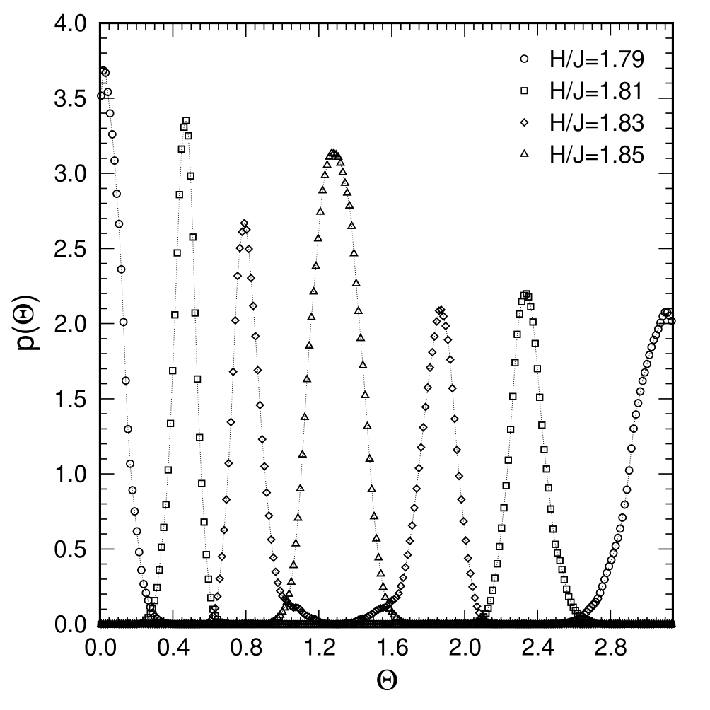
Figure 7: Histograms for the probability of the tilt angle $p(\Theta)$ for the XXZ antiferromagnet with a competing single–ion anisotropy, $D/J=0.2$, at $k_{B}T/J=0.2$, at the fields given in the inset. Lattices with $80^{2}$ spins are simulated. Note that the area under the curve has been normalised to be one.

In the BC phase the dominant interrelated tilt angles are changing continuously, at fixed low temperature, with the field. In fact, this behaviour is displayed by the probability function $p(\Theta)$, as illustrated in Fig. 7 for the global (sublattice) spin orientations. By increasing the field, at $k_{B}T/J=0.2$, the peak positions correspond first to the AF structure, shifting gradually towards each other, reflecting BC structures, and finally collapsing in one peak characterising the SF phase.

As seen in Fig. 5, the extent of the BC phase shrinks with increasing temperature. Eventually, the BC phase may terminate at a tetracritical point LF ; Bruce ; Aharony ; Mukamel ; Domany , where the AF, SF, BC, and paramagnetic phases meet. Because the phase boundaries seem to meet there with common tangents, we give here only a rough estimate for the case depicted in Fig. 5 ($D/J=0.2$ and $\Delta=0.8$), $k_{B}T_{tetra}/J=0.35\pm 0.05$. A more precise location and an analysis of its critical properties seem to require enormous computational efforts.

3.2 Anisotropic XY antiferromagnet

Finally, let us consider the anisotropic XY model, setting the exchange anisotropy $\Delta$= 0.8. Its phase diagram is depicted in Fig.8.

Figure 8: Phase diagram of the anisotropic XY model with $\Delta=0.8$.

The topology of the phase diagram looks like in the XXZ case Holt1 ; Zhou1 ; Holt2 . The AF and SF boundary lines approach each other very closely near the maximum of the AF phase boundary in the $(T,H)$–plane. Accordingly, at low temperatures, there seems to be either a direct transition between the AF and SF phases, or two separate transitions with an extremely narrow intervening phase may occur. At zero temperature and $H=H_{c1}(=2.4J)$, the highly degenerate ground state comprises SF, AF, and bidirectional structures.

Away from that intriguing transition region, see Fig. 8, one expects the transitions between the paramagnetic and the AF as well as the SF phases to be in the Ising universality class, because in the SF phase of the XY antiferromagnet, there is just one ordering component, the $y$–component. This consideration is confirmed by the Monte Carlo data for the specific heat (where the peak at the AF phase boundary gets rather weak on approach to the transition region) and for the staggered susceptibilities. The quantities exhibit critical behaviour of Ising–type, as follows from the corresponding effective exponents describing size dependences of the various peak heights.

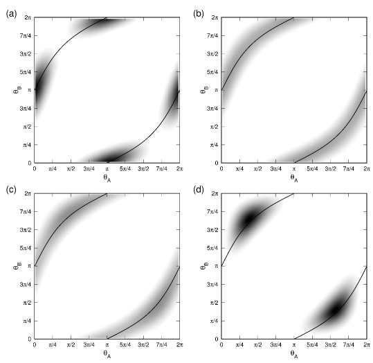
Figure 9: Probability $p_{2}(\theta_{A},\theta_{B})$ for the anisotropic XY antiferromagnet with $\Delta$= 0.8 for a system with $100\times 100$ lattice sites near the transition region between the AF and SF phases at $k_{B}T/J=0.4$ and $H/J=$ (a) 2.40, (b) 2.4136, (c) 2.4138, and (d) 2.43. $p_{2}(\theta_{A},\theta_{B})$ is proportional to the grayscale. The superimposed solid line depicts the relation between the two tilt angles in the ground state.

In the transition region of the AF and SF phases, BD fluctuations dominate, as one may conveniently infer from the (local) probability distribution $p_{2}(\Theta_{A},\Theta_{B})$ for finding the two tilt angles at neighbouring sites, i.e. for the two different sublattices. Typical results are depicted in Fig. 9, showing the behaviour of $p_{2}$ in a grayscale representation, at fixed temperature, $k_{B}T/J=0.4$ and different fields, somewhat below and above the, possibly, two closeby transitions as well as in their immediate vicinity. Indeed, at the low field, see Fig. 9(a), one finds a distribution corresponding to the AF phase, with peaks at $\Theta_{A/B}=0,\pi$. At the high field, Fig. 9(d), there is a distribution typical for the SF phase, with peaks at the spin–flop tilt angle. Note that the local maxima in $p_{2}$ follow closely the line describing the dependence of the two tilt angles in the degenerate ground state, eq. (6), albeit the probability of these BD structures is low compared to those of the AF and SF, resp., structures, see Figs. 9(a) and 9(d). In other words, thermal fluctuations driving the system away from the AF or SF structures are rather weak and, predominantly, of BD type.

In the immediate vicinity of the transitions, see Figs. 9(b) and 9(c), the BD fluctuations and structures clearly dominate. Now, all those degenerate bidirectional structures occur simultaneously with (almost) equal probability, i.e. along the line of maxima $p_{2}$ is (almost) constant. Actually, it is also interesting to monitor the time evolution of Monte Carlo configurations and of the probability $p(\Theta)$ in those configurations. One notices that at a given time of the simulation a concrete combination of interrelated tilt angles prevails. As Monte Carlo time evolves, other combinations in accordance with the ground state degeneracy prevail, leading to the behaviour depicted in Fig. 9. Obviously, this is is marked contrast to the situation in the ordered biconical phase at fixed field and temperature. There, after equilibration, just one combination of tilt angles seems to dominate during the entire simulation, see Fig. 7.

Note that in the transition region at higher temperatures, analysing systems of fixed size, say, $L=100$ (see Fig. 9), the various BD structures tend to occur simultaneously in a single MC configuration. Thence, for each configuration, $p(\Theta)$ has a shape quite similar to that in the degenerate ground state. This observation may be explained by a smaller correlation length. Typically, when increasing the system size, the region of (almost) constant values of $p_{2}$ along the line of local maxima shrinks somewhat. Certainly, further systematic studies of the time scales and temperature as well as size dependences related to the BD structures would be desirable.

Critical phenomena in the transition region between the AF and SF phases have been studied also by analysing effective exponents. We did that for the staggered susceptibilities and the specific heat. Results are compatible with Ising–type criticality, but rather large corrections to scaling had to be presumed. For example, at $H/J=2.44$ and $0.54<k_{B}T/J<0.57$, see Fig. 8, the effective critical exponents for describing the size–dependences of the peak height for the staggered susceptibilities are about 1.8 to 1.85, largely independent of system size. The supposedly rather strong corrections to scaling may be due to very large correlation lengths in that region, and the asymptotics may be reached only for very large systems.

In any event, the simulational data seem to suggest for the anisotropic XY antiferromagnet the existence of an extremely narrow, disordered phase, intervening between the AF and SF phases, like in the XXZ case Holt1 ; Zhou1 . That intermediate phase is dominated by all the, in the ground state completely degenerate, bidirectional fluctuations.

4 Summary

In this article, we studied two variants of the XXZ antiferromagnet in a field along the easy axis on a square lattice, by, firstly, adding a single–ion anisotropy, and by, secondly, reducing the number of spin components to two, yielding the anisotropic XY antiferromagnet. Large–scale Monte Carlo simulations have been performed, augmented by ground state calculations.

Adding a single–ion anisotropy has a drastic impact both on ground state properties and the phase diagram. Biconical structures, leading to a highly degenerate ground state in the XXZ antiferromagnet, are either suppressed, when the single–ion anisotropy fosters the uniaxial exchange anisotropy, or their degeneracy will be lifted by stabilising them successively with changing field, when the single–ion anisotropy introduces a planar anisotropy. In the former case, we observe, at low temperatures a direct first–order transition between the AF to SF phases, while in the other case, an ordered biconical phase emerges, separating the AF and SF phases. The situation in the XXZ case without single–ion anisotropy, where a narrow disordered phase with biconical fluctuations separates the AF and SF phases, interpolates in between these two scenarios with single–ion anisotropies of different sign.

When the uniaxiality of the antiferromagnet is solely due to a single–ion anisotropy, i.e. when the exchange couplings are isotropic, no biconical structures occur as ground states.

Ground state properties and the phase diagram of the anisotropic XY antiferromagnet are observed to resemble rather closely those of the XXZ antiferromagnet. There is a highly degenerate ground state, at which non–collinear structures of bidirectional type become stable. These degenerate bidirectional structures prevail at low temperatures in the transition region between the AF and SF phases, leading, presumably, to a very narrow intervening disordered phase.

We conclude that ground state properties and phase diagrams of classical uniaxially anisotropic antiferromagnets in two dimensions depend crucially on the form of the anisotropy terms, supporting or suppressing non–collinear structures of biconical or bidirectional type.

We should like to thank especially A. Aharony, G. Bannasch, K. Binder, D. P. Landau, A. Pelissetto, and E. Vicari for useful correspondence, information, remarks, and discussions. We gratefully acknowledge financial support by the Deutsche Forschungsgemeinschaft under grant SE324/4.

References

- (1) M. Matsuda, K. M. Kojima, Y. J. Uemura, J. L. Zarestky, K. Nakajima, K. Kakurai, T. Yokoo, S. M. Shapiro, and G. Shirane, Phys. Rev. B 57, 11467 (1998).
- (2) U. Ammerahl, B. Büchner, C. Kerpen, R. Gross, and A. Revcolevschi, Phys. Rev. B 62, R3592 (2000).
- (3) W. Selke, V. L. Pokrovsky, B. Büchner, and T. Kroll, Eur. Phys. J. B 30, 83 (2002); M. Holtschneider and W. Selke, Phys. Rev. E 68, 026120 (2003).
- (4) M. Matsuda, K. Kakurai, J. E. Lorenzo, L. P. Regnault, A. Hiess, and G. Shirane, Phys. Rev. B 68, 060406(R) (2003).
- (5) T. Kroll, R. Klingeler, J. Geck, B. Büchner, W. Selke, M. Hücker, and A. Gukasov, J. Magn. Magn. Mat. 290, 306 (2005).
- (6) M. Uehara, N. Motoyama, M. Matsuda, H. Eisaki, and J. Akimitsu, in: A. V. Narlikar (Ed.), Frontiers in Magnetic Materials, Springer (2005).
- (7) T. Vuletić, B. Korin-Hamzić, T. Ivek, S. Tomić, B. Gorshunov, M. Dressel, and J. Akimitsu, Phys. Rep. 428, 169 (2006).
- (8) U. Schwingenschlögl and C. Schuster, Europhys. Lett. 79, 27003 (2007); Phys. Rev. Lett. 99, 237206 (2007).
- (9) B. D. Gaulin, T. E. Mason, M. F. Collins, and J. Z. Larese, Phys. Rev. Lett. 62, 1380 (1989).
- (10) R. A. Cowley, A. Aharony, R. J. Birgeneau, R. A. Pelcovits, G. Shirane, and T. R. Thurston, Z. Phys. B 93, 5 (1993).
- (11) R. J. Christianson, R. L. Leheny, R. J. Birgeneau, and R. W. Erwin, Phys. Rev. B 63, 140401(R) (2001).
- (12) M. G. Pini, A. Rettori, P. Betti, J. S. Jiang, Y. Ji, S. G. E. te Velthuis, G. P. Felcher, and S. D. Bader, J. Phys.: Condens. Matter 19, 136001 (2007).
- (13) R. Leidl and W. Selke, Phys. Rev. B 70, 174425 (2004); Phys. Rev B 69, 056401 (2004).
- (14) M. Holtschneider, W. Selke, and R. Leidl, Phys. Rev. B 72, 064443 (2005).
- (15) C. Zhou, D. P. Landau, and T. C. Schulthess, Phys. Rev. B 74, 064407 (2006).
- (16) R. Leidl, R. Klingeler, B. Büchner, M. Holtschneider, and W. Selke, Phys. Rev. B 73, 224415 (2006).
- (17) M. Holtschneider, S. Wessel, and W. Selke, Phys. Rev. B 75, 224417 (2007).
- (18) A. Pelissetto and E. Vicari, Phys. Rev. B 76, 024436 (2007).
- (19) C. Zhou, D. P. Landau, and T. C. Schulthess, Phys. Rev. B 76, 024433 (2007).
- (20) M. Holtschneider and W. Selke, Phys. Rev. B 76, 220405(R) (2007).
- (21) K. Binder and D. P. Landau, Phys. Rev. B 13, 1140 (1976); D. P. Landau and K. Binder, Phys. Rev. B 24, 1391 (1981).
- (22) R. van de Kamp, M. Steiner and H. Tietze-Jaensch, Physica B 241-243, 570 (1997).
- (23) G. Schmid, S. Todo, M. Troyer, and A. Dorneich, Phys. Rev. Lett. 88, 167208 (2002).
- (24) R. Costa and W. Pires, J. Mag. Mag. Mat. 262, 316 (2003).
- (25) D. R. Nelson, J. M. Kosterlitz, and M. E. Fisher, Phys. Rev. Lett. 33, 813 (1974).
- (26) M. E. Fisher and D. R. Nelson, Phys. Rev. Lett. 32, 1350 (1974).
- (27) J. M. Kosterlitz, M. E. Fisher, and D. R. Nelson, Phys. Rev. B 13, 412 (1976).
- (28) N. D. Mermin and H. Wagner, Phys. Rev. Lett. 17, 1133 (1966).
- (29) H. Matsuda and T. Tsuneto, Prog. Theoret. Phys. Suppl. 46, 411 (1970).
- (30) K.-S. Liu and M. E. Fisher, J. Low. Temp. Phys. 10, 655 (1973).
- (31) F. Wegner, Solid State Commun. 12, 785 (1973).
- (32) J. M. Kosterlitz and D. J. Thouless, J. Phys. C 6, 1181 (1973).
- (33) M. Holtschneider, PhD thesis, RWTH Aachen (2007).
- (34) K. Binder, Z. Phys. B 43, 119 (1981); Phys. Rev. Lett. 47, 693 (1981).
- (35) A. D. Bruce and A. Aharony, Phys. Rev. B 11, 478 (1975).
- (36) A. Aharony, J. Stat. Phys. 110, 659 (2003).
- (37) D. Mukamel, Phys. Rev. B 14, 1303 (1976).
- (38) E. Domany and M. E. Fisher, Phys. Rev. B 15, 3510 (1977).