q-deformed statistical-mechanical property in the dynamics of trajectories en route to the Feigenbaum attractor

Abstract

We demonstrate that the dynamics towards and within the Feigenbaum attractor combine to form a $q$-deformed statistical-mechanical construction. The rate at which ensemble trajectories converge to the attractor (and to the repellor) is described by a $q$-entropy obtained from a partition function generated by summing distances between neighboring positions of the attractor. The values of the $q$-indices involved are given by the unimodal map universal constants, while the thermodynamic structure is closely related to that formerly developed for multifractals. As an essential component in our demonstration we expose, in great detail, the features of the dynamics of trajectories that either evolve towards the Feigenbaum attractor or are captured by its matching repellor. The dynamical properties of the family of periodic superstable cycles in unimodal maps are seen to be key ingredients for the comprehension of the discrete scale invariance features present at the period-doubling transition to chaos. Elements in our analysis are the following. (i) The preimages of the attractor and repellor of each of the supercycles appear entrenched into a fractal hierarchical structure of increasing complexity as period doubling develops. (ii) The limiting form of this rank structure results in an infinite number of families of well-defined phase-space gaps in the positions of the Feigenbaum attractor or of its repellor. (iii) The gaps in each of these families can be ordered with decreasing width in accordance with power laws and are seen to appear sequentially in the dynamics generated by uniform distributions of initial conditions. (iv) The power law with log-periodic modulation associated with the rate of approach of trajectories towards the attractor (and to the repellor) is explained in terms of the progression of gap formation. (v) The relationship between the law of rate of convergence to the attractor and the inexhaustible hierarchy feature of the preimage structure is elucidated. (vi) A “mean field” evaluation of the atypical partition function, a thermodynamic interpretation of the time evolution process, and a crossover to ordinary exponential statistics are given. We make clear the dynamical origin of the anomalous thermodynamic framework existing at the Feigenbaum attractor.

Key words: $q$-statistics, Feigenbaum attractor, supercycles, convergence to attractor

PACS: 05.90.+m, 05.45.Ac, 05.45.Df

I Introduction

A fundamental question in statistical physics is whether the structure of ordinary equilibrium statistical mechanics falters when its fundamental properties, phase-space mixing and ergodicity, breakdown. The chaotic dynamics displayed by dissipative nonlinear systems, even those of low dimensionality, possesses these two crucial conditions, and acts in accordance with a formal structure analogous to that of canonical statistical mechanics, in which thermodynamic concepts meet their dynamical counterparts beck1 . At the transition between chaotic and regular behavior, classically represented by the Feigenbaum attractor beck1 , the Lyapunov exponent vanishes and chaotic dynamics turns critical. Trajectories cease to be ergodic and mixing; they retain memory of their initial positions and fluctuate according to complex deterministic patterns mori1 . Under these conditions it is of interest to check up whether the statistical-mechanical structure subsists, and if so, examine if it is unchanged or if it has acquired a new form.

With this purpose in mind, the exploration of possible limits of validity of the canonical statistical mechanics, an ideal model system is a one-dimensional map at the transition between chaotic and regular behavior, represented by well-known critical attractors, such as the Feigenbaum attractor. So far, recent studies robledo1 have concentrated on the dynamics inside the attractor and have revealed that these trajectories obey remarkably rich scaling properties not known previously at this level of detail robledo2 . The results are exact and clarify robledo2 the relationship between the original modification politi1 ; mori1 of the thermodynamic approach to chaotic attractors thermo1 ; thermo2 ; thermo3 for this type of incipiently chaotic attractor, and some aspects of the $q$-deformed statistical mechanical formalism note1 ; robledo3 ; tsallis1 . The complementary part of the dynamics, that of advance on the way to the attractor, has, to our knowledge, not been analyzed, nor understood, with a similar degree of thoroughness. The process of convergence of trajectories into the Feigenbaum attractor poses several interesting questions that we attempt to answer here and elsewhere robledo00 based on the comprehensive knowledge presented below. Prominent amongst these questions is the nature of the connection between the two sets of dynamical properties, within and outside the attractor. As it turns out, these two sets of properties are related to each other in a statistical-mechanical manner, i.e. the dynamics at the attractor provides the configurations in a partition function while the approach to the attractor is described by an entropy obtained from it. As we show below, this statistical-mechanical property conforms to a $q$-deformation note1 of the ordinary exponential weight statistics.

Trajectories inside the attractor visit positions forming oscillating log-periodic patterns of ever increasing amplitude. However, when the trajectories are observed only at specified times, positions align according to power laws, or $q$-exponential functions that share the same $q$-index value robledo2 ; robledo3 . Further, all such sequences of positions can be shifted and seen to collapse into a single one by a rescaling operation similar to that observed for correlations in glassy dynamics, a property known as “aging” robledo3 ; robledo4 . The structure found in the dynamics is also seen to consist of a family of Mori’s $q$-phase transitions mori1 , via which the connection is made between the modified thermodynamic approach and the $q$-statistical property of the sensitivity to initial conditions robledo2 ; robledo3 . On the other hand, a foretaste of the nature of the dynamics outside the critical attractor can be appreciated by considering the dynamics towards the so-called superstable cycles, or supercycles, the family of periodic attractors with Lyapunov exponents that diverge towards minus infinity. This infinite family of attractors has as accumulation point the transition to chaos, which for the period-doubling route is the Feigenbaum attractor. As described below, the basins of attraction for the different positions of the cycles develop fractal boundaries of increasing complexity as the period-doubling structure advances towards the transition to chaos. The fractal boundaries, formed by the preimages of the repellor, display hierarchical structures organized according to exponential clusterings that manifest in the dynamics as sensitivity to the final state and transient chaos. The hierarchical arrangement expands as the period of the supercycle increases.

To observe the general procedure followed by trajectories to reach the attractors, and their complementary repellors, we consider an ensemble of uniformly distributed initial conditions $x_{0}$ spanning the entire phase space interval. We find that this is a highly structured process encoded in sequences of positions shared by as many trajectories with different $x_{0}$. Clearly, there is always a natural dynamical ordering in the $x_{0}$ as any trajectory of length $t$ contains consecutive positions of other trajectories of lengths $t-1$, $t-2$, etc. with initial conditions $x_{0}^{\prime}$, $x_{0}^{\prime\prime}$, etc. that are images under repeated map iterations of $x_{0}$. In the case of the Feigenbaum attractor the initial conditions form two sets, dense in each other, of preimages of each the attractor and the repellor. There is an infinite-level structure within these sets that, as we shall see, is reflected by the infinite number of families of phase-space gaps that complement the multifractal layout of both attractor and repellor. These families of gaps appear sequentially in the dynamics, beginning with the largest and followed by other sets consisting of continually increasing elements with decreasing widths. The number of gaps in each set of comparable widths increases as $2^{k}$, $k=0,1,\ldots$ and their widths can be ordered according to power laws of the form $\alpha^{-k}$, where $\alpha$ is Feigenbaum’s universal constant $\alpha\simeq 2.5091$. We call $k$ the order of the gap set. Furthermore, by considering a fine partition of phase-space, we determine the overall rate of approach of trajectories towards the attractor (and to the repellor). This rate is measured by the fraction of bins $W(t)$ still occupied by trajectories at time $t$ lyra1 . The power law with log-periodic modulation displayed by $W(t)$ lyra1 is explained in terms of the progression of gap formation, and its self-similar features are seen to originate in the unlimited hierarchy feature of the preimage structure.

Before proceeding to give details in the following sections of the aforementioned dynamics, we recall basic features of the bifurcation forks that form the period-doubling cascade sequence in unimodal maps, epitomized by the logistic map $f_{\mu}(x)=1-\mu x^{2}$, $-1\leq x\leq 1$, $0\leq\mu\leq 2$ schuster1 ; beck1 . The superstable periodic orbits of lengths $2^{N}$, $N=1,2,3,\ldots$, are located along the bifurcation forks, i.e. the control parameter value $\mu=\overline{\mu}_{N}<\mu_{\infty}$ for the superstable $2^{N}$-attractor is that for which the orbit of period $2^{N}$ contains the point $x=0$, where $\mu_{\infty}=1.401155189\ldots$ is the value of $\mu$ at the period-doubling accumulation point. The positions (or phases) of the $2^{N}$-attractor are given by $x_{m}=f_{\overline{\mu}_{N}}^{(m)}(0)$, $m=1,2,\ldots,2^{N}$. Notice that infinitely many other sequences of superstable attractors appear at the period-doubling cascades within the windows of periodic attractors for values of $\mu>$ $\mu_{\infty}$. Associated with the $2^{N}$-attractor at $\mu=\overline{\mu}_{N}$ there is a $(2^{N}-1)$-repellor consisting of $2^{N}-1$ positions $y_{m}$, $m=1,2,\ldots,2^{N}-1$. These positions are the unstable solutions $\left|df_{\overline{\mu}_{N}}^{(2^{k})}(y)/dy\right|<1$ of $y=f_{\overline{\mu}_{N}}^{(2^{k})}(y)$, $k=0,1,2,\ldots,N-1$. The first, $k=0$, originates at the initial period-doubling bifurcation, the next two, $k=1$, start at the second bifurcation, and so on, with the last group of $2^{N-1}$, $k=N-1$, stemming from the $N-1$ bifurcation. We find it useful to order the repellor positions, or simply, repellors, present at $\mu=\overline{\mu}_{N}$, according to a hierarchy or tree, the “oldest” with $k=0$ up to the most “recent” ones with $k=N-1$. The repellors’ order is given by the value of $k$. Finally, we define the preimage $x^{(j)}$ of order $j$ of position $x$ to satisfy $x=h^{(j)}(x^{(j)})$ where $h^{(j)}(x)$ is the $j$-th composition of the map $h(x)\equiv f_{\overline{\mu}_{N}}^{(2^{N-1})}(x)$. We have omitted reference to the $2^{N}$-cycle in $x^{(j)}$ to simplify the notation. The interval lengths or diameters $d_{N,m}$ are measured when considering the superstable periodic orbits of lengths $2^{N}$. The $d_{N,m}$ are defined (here) as the (positive) distances of the elements $x_{m}$, $m=0,1,2,\ldots,2^{N}-1$, to their nearest neighbors $f_{\overline{\mu}_{N}}^{(2^{N-1})}(x_{m})$, i.e.

$$d_{N,m}\equiv\left|f_{\overline{\mu}_{N}}^{(m+2^{N-1})}(0)-f_{\overline{\mu}_{N}}^{(m)}(0)\right|.$$ (1)

For large $N$, $d_{N,0}/d_{N+1,0}\simeq\alpha$. We present explicit results for the logistic map, which has a quadratic maximum, but the results are easily extended to unimodal maps with general nonlinearity $z>1$.

Central to our discussion is the following broad property: Time evolution at $\mu_{\infty}$ from $t=0$ up to $t\rightarrow\infty$ traces the period-doubling cascade progression from $\mu=0$ up to $\mu_{\infty}$. Not only is there a close resemblance between the two developments but also quantitative agreement. For instance, the trajectory inside the Feigenbaum attractor with initial condition $x_{0}=0$, the $2^{\infty}$-supercycle orbit, takes positions $x_{t}$ such that the distances between appropriate pairs of them reproduce the diameters $d_{N,m}$ defined from the supercycle orbits with $\overline{\mu}_{N}<\mu_{\infty}$. See Fig. 1, where the absolute value of positions and logarithmic scales are used to illustrate the equivalence. This property has been key to obtain rigorous results for the sensitivity to initial conditions for the Feigenbaum attractor robledo1 ; robledo3 .

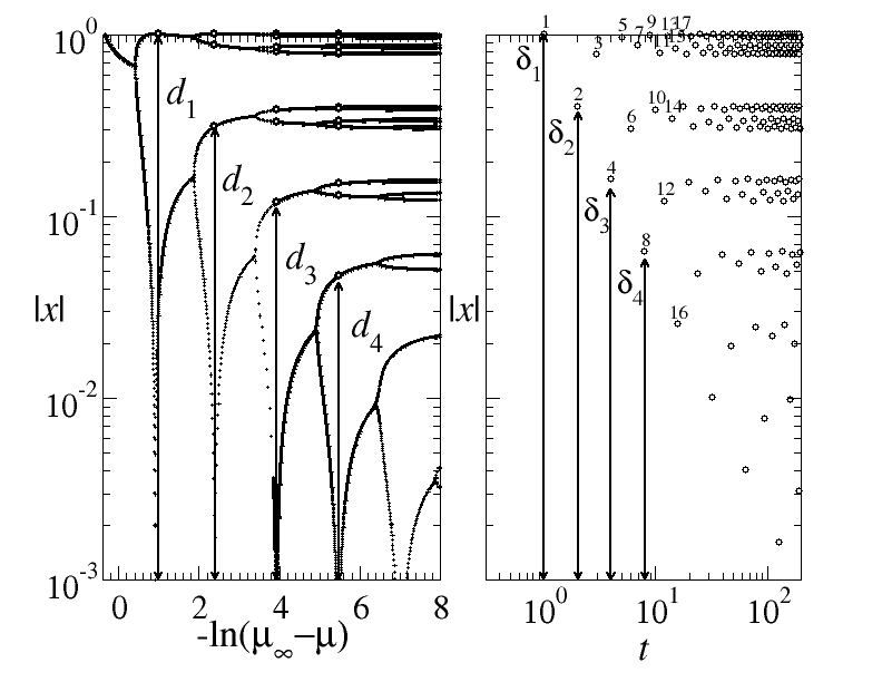
Figure 1:  Left panel: Absolute value of attractor positions for the logistic map ${\small f}_{\mu}{\small(x)}$ in logarithmic scale as a function of the logarithm of the control parameter difference ${\small\mu}_{\infty}{\small-\mu}$. Right panel: Absolute value of trajectory positions for the logistic map ${\small f}_{\mu}{\small(x)}$ at ${\small\mu}_{\infty}$ with initial condition ${\small x}_{0}{\small=0}$ in logarithmic scale as a function of the logarithm of time $t$, also shown by the numbers close to the circles. The arrows indicate the equivalence between the diameters $\delta_{N}$ in the left panel, and position differences $\delta_{N}$ with respect to ${\small x}_{0}{\small=0}$ in the right panel.

The layout of the rest of this paper is the following. In Sec. II we present the dynamical properties of the family of supercycles, describing their preimage structure, final state sensitivity and transient chaos. Details of the superstrong insensitivity to initial conditions displayed by these attractors are given as an Appendix. In Sec. III we make use of the results of the previous section to describe the dynamical properties of approach to the Feigenbaum attractor. We provide details of its preimage structure, the sequential opening of phase-space gaps, and the scaling for the trajectories’ rate of convergence to the attractor (and repellor). In Sec. IV we explain the aforesaid statistical-mechanical structure lying beneath the dynamics of an ensemble of trajectories en route to the Feigenbaum attractor (and repellor). In Sec. V we summarize our results.

II Hierarchical properties in the dynamics of supercycle attractors

To obtain dynamical properties with previously unstated detail we determined the organization of the entire set of trajectories as generated by all possible initial conditions. We find that the paths taken by the full set of trajectories in their way to the supercycle attractors (or to their complementary repellors) are far from unstructured. The preimages of the attractor of period $2^{N}$, $N=1,2,3,\ldots$ are distributed into different basins of attraction, one for each of the $2^{N}$ phases (positions) that compose the cycle. When $N\geq 2$ these basins are separated by fractal boundaries whose complexity increases with increasing $N$. The boundaries consist of the preimages of the corresponding repellor and their positions cluster around the $2^{N}-1$ repellor positions according to an exponential law. As $N$ increases the structure of the basin boundaries becomes more involved. That is, the boundaries for the $2^{N}$ cycle develop new features around those of the previous $2^{N-1}$ cycle boundaries, with the outcome that a hierarchical structure arises, leading to embedded clusters of clusters of boundary positions, and so forth.

The dynamics associated with families of trajectories always displays a distinctively concerted order that reflects the repellor preimage boundary structure of the basins of attraction. That is, each trajectory has an initial condition that is identified as an attractor (or repellor) preimage of a given order, and this trajectory necessarily follows the steps of other trajectories with initial conditions of lower preimage order belonging to a given chain or pathway to the attractor (or repellor). This feature gives rise to transient chaotic behavior different from that observed at the last stage of approach to the attractor. When the period $2^{N}$ of the cycle increases the dynamics becomes more involved with increasingly more complex stages that reflect the preimage hierarchical structure. As a final point, shown in the appendix, in the closing part of the last leg of the trajectories an ultra-rapid convergence to the attractor is observed, with a sensitivity to initial conditions that decreases as an exponential of an exponential in time. In relation to this we find that there is a functional composition renormalization group (RG) fixed-point map associated with the supercycle attractor, and this can be expressed in closed form by the same kind of $q$ -exponential function found for both the pitchfork and tangent bifurcation attractors robledo5 ; robledo6 , like that originally derived by Hu and Rudnick for the latter case hu1 .

II.1 Preimage structure of supercycle attractors

The core source of our description of the dynamics towards the supercycle attractors is a measure of the relative “time of flight” $t_{f}(x_{0})$ for a trajectory with initial condition $x_{0}$ to reach the attractor. The function $t_{f}(x_{0})$ is obtained for an ensemble representative of all initial conditions $-1\leq x_{0}\leq 1$. This comprehensive information is determined through the numerical realization of every trajectory, up to a small cutoff $\varepsilon>0$ at its final stage. The cutoff $\varepsilon$ considers a position $x_{f}\leq x_{m}\pm\varepsilon$ to be effectively the attractor phase $x_{m}$. This, of course, introduces an approximation to the real time of flight, which can be arbitrarily large for those $x_{0}$ close to a repellor position $y_{m}$ or close to any of its infinitely many preimages, $x_{m}^{(j)}$, $j=1,2,\ldots$, $N\geq 2$. In such cases the finite time $t_{f}(x_{0};\varepsilon)$ can be seen to diverge $t_{f}\rightarrow\infty$ as $x_{0}\rightarrow y_{m}$ and $\varepsilon\rightarrow 0$. As a simple illustration, in Fig. 2 we show the time of flight $t_{f}(x_{0})$ for the period $2$ supercycle at $\mu=\overline{\mu}_{1}$ with $\varepsilon=10^{-9}$ together with the twice-composed map $f_{\overline{\mu}_{1}}^{(2)}(x)$ and a few representative trajectories. We observe two peaks in $t_{f}(x_{0};\varepsilon)$ at $y_{1}=(-1+\sqrt{1+4\overline{\mu}_{1}})/2\overline{\mu}_{1}\simeq 0.6180340\ldots$, the fixed-point repellor and at its (only) preimage $x_{1}^{(1)}=-y_{1}$, where $y_{1}=f_{\overline{\mu}_{1}}^{(2)}(x_{1}^{(1)})$. Clearly, there are two basins of attraction each for the two positions or phases, $x_{1}=0$ and $x_{2}=1$, of the attractor. For the former it is the interval $x_{1}^{(1)}<x_{0}<y_{1}$, whereas for the second one it consists of the intervals $-1\leq x_{0}<x_{1}^{(1)}$ and $y_{1}<x_{0}\leq 1$. The multiple-step structure of $t_{f}(x_{0})$, of four time units each step, reflects the occurrence of intervals of initial conditions with common attractor phase preimage order $k$.

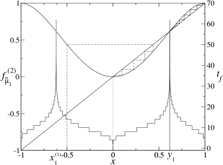
Figure 2: Left axis: The twice iterated map ${\small f}_{\overline{\mu}_{1}}^{(2)}{\small(x)}$, with $\overline{\mu}_{1}{\small=1}$ (gray line). Right axis: Time of flight ${\small t}_{f}{\small(x)}$, the number of iterations necessary for a trajectory with initial condition at ${\small x}$ to reach an attractor position. The values of ${\small x}$ near the high spikes correspond to initial conditions very close to the repellor and its preimage. We present three example trajectories (and the ${\small y=x}$ line as an aid to visualize them): The dotted line shows a trajectory that starts at the attractor position ${\small x=0}$ and remains there. The solid line is a trajectory starting near the repellor at ${\small y}_{{\small 1}}$, and after a large number of iterations reaches the attractor position ${\small x=1}$. Finally, the dash-dotted line is an orbit starting at ${\small x=0.5}$ that in just a few iterations reaches ${\small x=0}$.

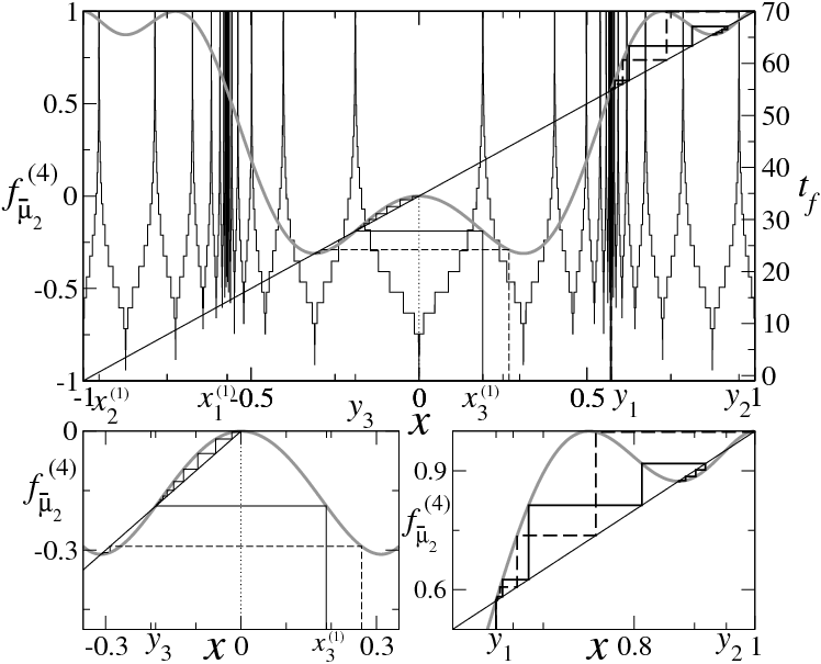
Figure 3: Same as Fig. 2 but for $f_{\overline{\mu}_{2}}^{(4)}(x)$, $\overline{\mu}_{2}\simeq{\small 1.31070264}$. Two orbits (solid bold and dashed bold lines) start very near each other and by the position ${\small y}_{{\small 1}}$ of the old repellor, although indistinguishable at the beginning they take very different subsequent paths to reach the attractor positions at ${\small x=1}$ and ${\small x\simeq 0.8734}$. See bottom right panel. Another two orbits (in dotted and solid lines) start at an attractor position ${\small x=1}$ and at a repellor preimage position, respectively. Finally, one more orbit (dashed line) starts at an intermediate initial condition and reaches very quickly the attractor position at ${\small x\simeq-0.310703}$. See bottom left panel.

For the next supercycle—period $4$—the preimage structure turns out to be a good deal more involved than the straightforward structure for $\overline{\mu}_{1}$. In Fig. 3 we show the times of flight $t_{f}(x_{0})$ for the $N=2$ supercycle at $\mu=\overline{\mu}_{2}$ with $\varepsilon=10^{-9}$, the map $f_{\overline{\mu}_{2}}^{(4)}(x)$ is superposed as a reference to indicate the four phases of the attractor (at $x_{1}=0$, $x_{2}=1$, $x_{3}\simeq-0.3107\ldots$, and $x_{4}\simeq 0.8734\ldots$) and the three repellor positions (at $y_{1}\simeq 0.5716635\ldots$, $y_{2}\simeq 0.952771\ldots$, and $y_{3}\simeq-0.189822\ldots$) In Fig. 3 there are also shown four trajectories each of which terminates at a different attractor phase. We observe a proliferation of peaks and valleys in $t_{f}(x_{0})$, actually, an infinite number of them, that cluster around the repellor at $y_{1}\simeq 0.5716635\ldots$ and also at its preimage at $x_{1}^{(1)}=-y_{1}$ (these are the positions at $\mu=\overline{\mu}_{2}$ of the “old” repellor and its preimage in the previous $N=1$ case). Notice that the steps in the valleys of $t_{f}(x_{0})$ are now eight time units each. The nature of the clustering of peaks (repellor phase preimages) and the bases of the valleys (attractor phase preimages) is revealed in Fig. 4 where we plot $t_{f}$ on a logarithmic scale for the variables $\pm(x-y_{1})$. There is an exponential clustering of the preimage structure around both the old repellor and its preimage. This scaling property is corroborated in Fig. 5 from which we obtain $x-y_{1}\simeq 7.5\times 10^{-5}\exp(0.80\,l)$, where $l=1,2,3,\ldots$ is a label for consecutive repellor preimages.

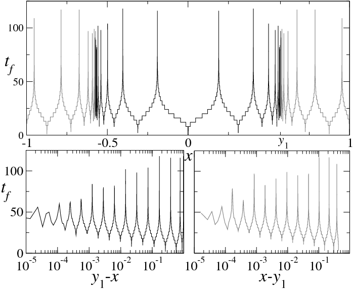
Figure 4: Top panel: Time of flight ${\small t}_{f}{\small(x)}$ for ${\small N=2}$ (as in Fig. 3), the black lines correspond to initial conditions that terminate at the attractor positions ${\small x=0}$ and ${\small x\simeq-0.310703}$, and the gray lines to trajectories ending at ${\small x=1}$ and ${\small x\simeq 0.8734}$. Right (left) bottom panel: Same as top panel, but plotted against the logarithm of ${\small x-y}_{{\small 1}}$ (${\small y}_{{\small 1}}{\small-x}$). It is evident that the peaks are arranged exponentially around the old repellor position ${\small y}_{{\small 1}}$, i.e., they appear equidistant on a logarithmic scale. See Fig. 5.

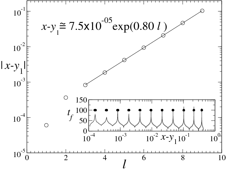
Figure 5: Corroboration of preimage exponential clustering around the repellor position ${\small y}_{{\small 1}}\simeq{\small 0.571663}$ when ${\small N=2}$ and $\overline{\mu}_{2}\simeq{\small 1.31070264}$. The variable ${\small l}$ labels consecutive equidistant peaks in the inset. The peaks correspond to preimages of the repellor. See text.

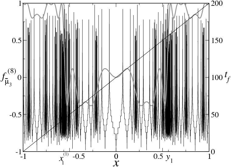
Figure 6: Same as Fig. 3 but for ${\small f}_{\overline{\mu}_{3}}^{(8)}{\small(x)}$, $\overline{\mu}_{3}{\small\simeq 1.38154748}$. Here ${\small y}_{{\small 1}}{\small=0.56264475}$.

A comparable leap in the complexity of the preimage structure is observed for the following—period $8$—supercycle. In Fig. 6 we show $t_{f}(x_{0})$ for the $N=3$ supercycle at $\mu=\overline{\mu}_{3}$ with $\varepsilon=10^{-9}$, together with the map $f_{\overline{\mu}_{2}}^{(8)}(x)$ placed as reference to facilitate the identification of the locations of the eight phases of the attractor, $x_{1}$ to $x_{8}$, and the seven repellor positions, $y_{1}$ to $y_{7}$. In addition to a huge proliferation of peaks and valleys in $t_{f}(x_{0})$, we observe now the development of clusters of clusters of peaks centered around the repellor at $y_{1}\simeq 0.5626447\ldots$ and its preimage at $x_{1}^{(1)}=-y_{1}$ (these are now the positions of the original repellor and its preimage for the $N=1$ case when $\mu=\overline{\mu}_{3}$). The steps in the valleys of $t_{f}(x_{0})$ have become 16 time units each. Similarly to the clustering of peaks (repellor phase preimages) and valleys (attractor phase preimages) for the previous supercycle at $\overline{\mu}_{2}$, the spacing arrangement of the new clusters of clusters of peaks is determined in Fig. 7 where we plot $t_{f}$ in a logarithmic scale for the variables $\pm(x-y_{1})$. In parallel to the previous cycle an exponential clustering of clusters of the preimage structure is found around both the old repellor and its preimage. This scaling property is quantified in Fig. 8 from which we obtain $x-y_{1}\simeq 8.8\times 10^{-5}\exp(0.84\,l),$ where $l=1,2,3,\ldots$ counts consecutive clusters.

Figure 7: Same as Fig. 4 but for ${\small N=3}$. The black lines correspond to initial conditions that terminate at any of the four attractor positions close or equal to ${\small x=0}$, and the gray lines to trajectories ending at any of the other four attractor positions close or equal to ${\small x=1}$. As the bottom panels show, on a logarithmic scale, in this case there are (infinitely) many clusters of peaks (repellor preimages) equidistant from each other.

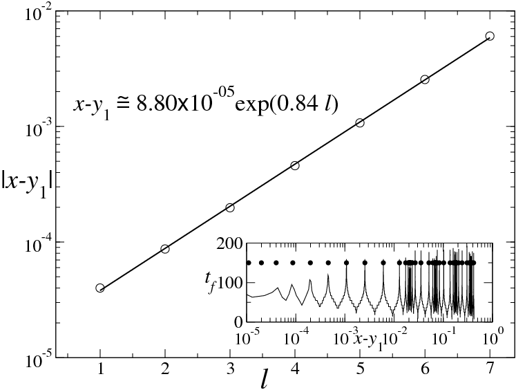
Figure 8: Same as Fig. 5 but for ${\small N=3}$.

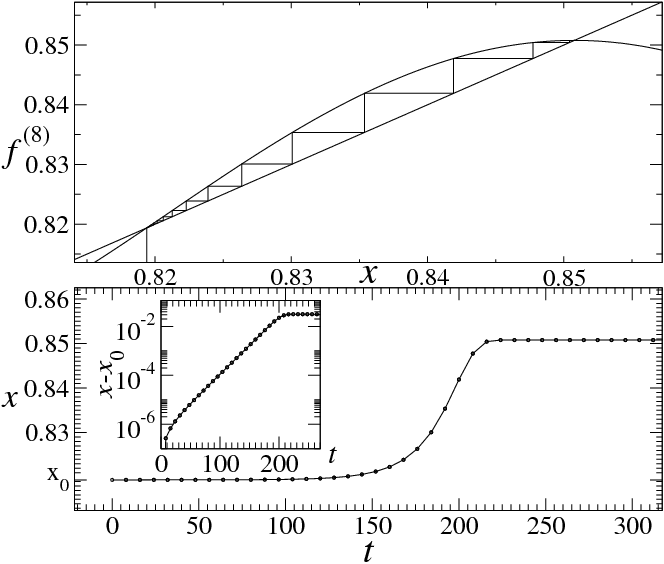
Figure 9: Top panel: Detail of the map ${\small f}_{\overline{\mu}_{3}}^{(8)}{\small(x)}$ and a trajectory in the proximity of the attractor position located at ${\small x\simeq 0.850780}$. The trajectory originated very close to the repellor position at ${\small x=0.819378}$. Bottom panel: The same trajectory of the eight-iterated map as a function of time ${\small t}$. Inset: Corroboration of the exponential nature of the trajectory after it leaves the repellor and before the final approach to the attractor position.

An investigation of the preimage structure for the next $N=4$ supercycle at $\mu=\overline{\mu}_{4}$ leads to another substantial increment in the complications of the structure of the preimages but with such density that is cumbersome to describe here. Nevertheless it is clear that the main characteristic in the dynamics is the development of a hierarchical organization of the preimage structure as the period $2^{N}$ of the supercycles increases.

II.2 Final state sensitivity and transient chaos

With the knowledge gained about the features displayed by the times of flight $t_{f}(x_{0})$ for the first few supercycles it is possible to determine and understand how the leading properties in the dynamics of approach to these attractors arise. The information contained in $t_{f}(x_{0})$ can be used to demonstrate in detail how the concepts of final state sensitivity grebogi1 —due to attractor multiplicity—and transient chaos beck1 —prevalent in the presence of repellors that coexist with periodic attractors—are realized in a given dynamics. Final state sensitivity is the consequence of fractal boundaries separating coexisting attractors. In our case there is always a single attractor but its positions or phases play an equivalent role grebogi2 . Transient chaos beck1 is due to fast separation in time of nearby trajectories by the action of a repellor and results in a sensitivity to initial conditions that grows exponentially up to a crossover time after which decay sets in. We describe how both properties result from an extremely ordered flow of trajectories towards the attractor. This order is imprinted by the preimage structure described above.

For the simplest supercycle at $\mu=\overline{\mu}_{1}$ there is trivial final state sensitivity as the boundary between the two basins of the phases, $x_{1}=0$ and $x_{2}=1$, consists only of the two positions $y_{1}\simeq 0.5716635\ldots$ and $x_{1}^{(1)}=-y_{1}$. See Fig. 2. Consider the length $\delta$ of a small interval around a given value of $x_{0}$ containing either $y_{1}$ or $x_{1}^{(1)}$, when $\delta\rightarrow 0$ any uncertainty as to the final phase of the trajectory disappears. It is also simple to verify that when $x_{0}$ is close to $y_{1}$ or $x_{1}^{(1)}$ the resulting trajectories increase their separation at initial and intermediate times displaying transient chaos in a straightforward fashion. In Fig. 9 we show the same type of transitory exponential sensitivity to initial conditions for a trajectory at $\mu=\overline{\mu}_{3}$ after it reaches a repellor position in the final journey towards the period $8$ attractor. This behavior is common to all periodic attractors when trajectories come near a repellor at the final leg of their journey.

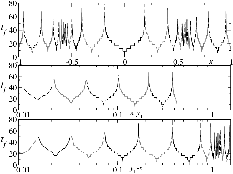
Figure 10: Time of flight ${\small t}_{f}{\small(x)}$ for ${\small N=2}$ (equivalent to Fig. 4). Different types of lines are used for different sub-basins of attraction that form the fractal boundary between the attractor positions. The black solid line corresponds to the attractor position ${\small x=0}$, the gray solid line to ${\small x=1}$, the dashed gray line to ${\small x\simeq-0.310703}$, and the dashed black line to ${\small x\simeq 0.873470}$. The sub-basins are separated in an alternating fashion by repellor preimages (peaks) and there are just two types of sub-basins depending on ${\small|x|}$ being larger or smaller than ${\small y}_{{\small 1}}$.

For $\mu=\overline{\mu}_{2}$ there are more remarkable properties arising from the more complex preimage structure. There is a concerted migration of initial conditions seeping through the boundaries between the four basins of attraction of the phases. These boundaries, shown in Fig. 10, form a fractal network of interlaced sub-basins separated from each other by two preimages of different repellor phases and have at their bottom a preimage of an attractor phase. Trajectories on one of these sub-basins move to the nearest sub-basin of its type (next-nearest neighbor in actual distance in Fig. 10) at each iteration of the map $f_{\overline{\mu}_{2}}^{(4)}$ (four time steps for the original map $f_{\overline{\mu}_{2}}$). The movement is always away from the center of the cluster at the old repellor position $y_{1}$ or at its preimage $x_{1}^{(1)}$ (located at the steepest slope inflection points of $f_{\overline{\mu}_{2}}^{(4)}$ shown in Fig. 3). Once a trajectory is out of the cluster (contained between the maxima and minima of $f_{\overline{\mu}_{2}}^{(4)}$ next to the mentioned inflection points) it proceeds to the basin of attraction of an attractor phase (separated from the cluster by the inflection points with gentler slope of $f_{\overline{\mu}_{2}}^{(4)}$ in Fig. 3) where its final stage takes place. When we consider a large ensemble of initial positions, distributed uniformly along all phase-space, the common journey towards the attractor displays an exceedingly ordered pattern. Each initial position $x_{0}$ within either of the two clusters of sub-basins is a preimage of a given order $k$ of a position in the main basin of attraction. Each iteration of $f_{\overline{\mu}_{2}}^{(4)}$ reduces the order of the preimage from $k$ to $k-1$, and the new position $x_{0}^{\prime}=f_{\overline{\mu}_{2}}^{(4)}(x_{0})$ replaces the initial position $x_{0}^{\prime}$ (a preimage of order $k-1$) of another trajectory that under the same time step has migrated to the initial position $x_{0}^{\prime\prime}$ (a preimage of order $k-2$) of another trajectory, and so on.

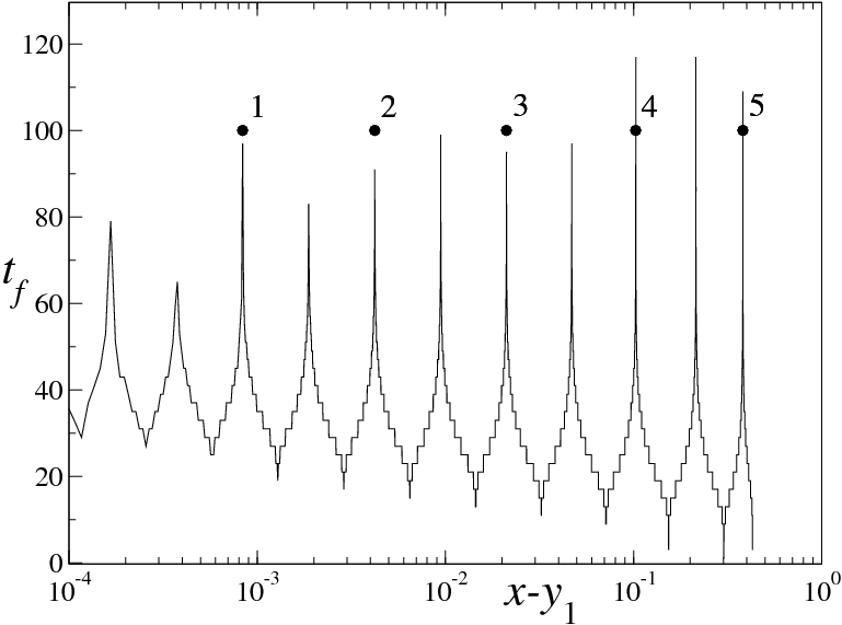
Figure 11: Evolution of an orbit starting very close to a peak (repellor preimage) inside a cluster when ${\small N=2}$, $\overline{\mu}_{2}\simeq{\small 1.31070264}$ and ${\small y}_{1}{\small=0.571663}$. (See Fig. 4.) The trajectory describes an exponential in time moving away from ${\small y}_{{\small 1}}$. In the figure, positions of the trajectory correspond to the black solid dots, and iterations correspond to the number associated with each dot.

It is clear that the dynamics at $\mu=\overline{\mu}_{2}$ displays sensitivity to the final state when the initial condition $x_{0}$ is located near the core of any of the two clusters of sub-basins at $y_{1}$ and $x_{1}^{(1)}$ that form the boundary of the attractor phases. Any uncertainty on the location of $x_{0}$ when arbitrarily close to these positions implies uncertainty about the final phase of a trajectory. There is also transient chaotic behavior associated to the migration of trajectories out of the cluster as a result of the organized preimage resettlement mentioned above. Indeed, the exponential disposition of repellor preimages shown in Fig. 5 is actually a realization of two trajectories with initial conditions in consecutive peaks of the cluster structure. Therefore, the exponential expression given in the previous section in relation to Fig. 5 can be rewritten as the expression for a trajectory $x_{\theta}\simeq x_{0}\exp(\lambda_{eff}\theta)$, with $x_{\theta}=x-y_{1}$, $x_{0}=$ $7.5\times 10^{-5}$, and $\lambda_{eff}=6.4$, where $\theta=1,2,3,\ldots$ Straightforward differentiation of $x_{\theta}$ with respect to $x_{0}$ yields an exponential sensitivity to initial conditions with positive effective Lyapunov coefficient $\lambda_{eff}$. See Fig. 11.

As can be anticipated, the dynamics of approach to the next supercycle at $\mu=\overline{\mu}_{3}$ can be explained by enlarging the description presented above for $\mu=\overline{\mu}_{2}$ with the additional features of its preimage structure already detailed in the preceding section. As in the previous case, trajectories with initial conditions $x_{0}$ located inside a cluster of sub-basins of the attractor phases will proceed to move out of it in the systematic manner described for the only two isolated clusters present when $\mu=\overline{\mu}_{2}$. However, now there is an infinite number of such clusters arranged into two bunches that group exponentially around the old repellor position $y_{1}$ and around its preimage $x_{1}^{(1)}$. See Figs. 6–8. Once such trajectories leave the cluster under consideration they enter into a neighboring cluster, and so forth, so that the trajectories advance out of these fractal boundaries through the prolonged process of migration out of the cluster of clusters before they proceed to the basins of the attraction of the eight phases of this cycle. In Fig. 12 we show one such trajectory in consecutive times $t=1,2,3,\ldots$ for the original map and also in multiples of time $t=2^{3},22^{3},32^{3},\ldots$. The logarithmic scale of the figure makes evident the retardation of each stage in the process. As when $\mu=\overline{\mu}_{2}$, it is clear that in the approach to the $\mu=\overline{\mu}_{3}$ attractor there is sensitivity to the final state and transitory chaotic sensitivity to initial conditions. Again, the exponential expression, given in the previous section associated with the preimage structure of clusters of clusters of sub-basins, shown in Fig. 8, can be interpreted as the expression of a trajectory of the form $x_{\theta}\simeq x_{0}\exp(\lambda_{eff}\theta)$. Differentiation of $x_{\theta}$ with respect to $x_{0}$ yields again an exponential sensitivity to initial conditions with positive effective Lyapunov coefficient $\lambda_{eff}$.

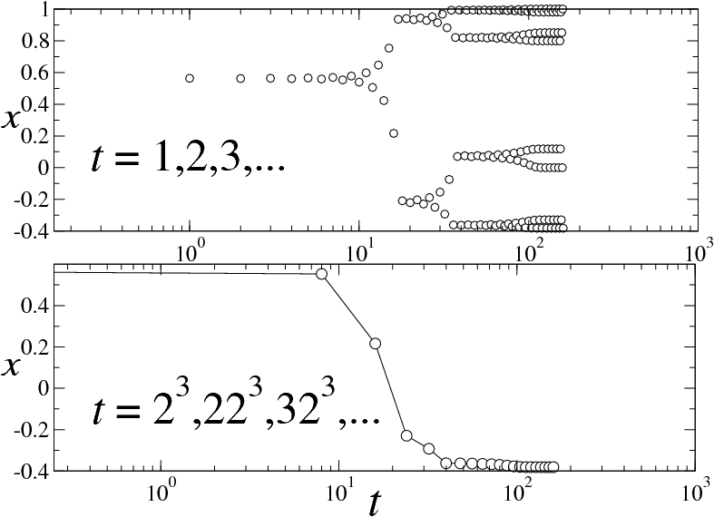
Figure 12: A trajectory for $\overline{\mu}_{3}{\small\simeq 1.38154748}$. Top panel: The circles are positions for consecutive times in the iterations of the map ${\small f}_{\overline{\mu}_{3}}{\small(x)}$. The orbit starts very close to the old (period 1) repellor ${\small y}_{{\small 1}}$, then moves close to a period 2 and subsequently to a period 4 repellor, until finally it arrives at the period 8 attractor. Bottom panel: Selection of a time subsequence of multiples of ${\small 2}^{3}$ shows the same trajectory as an evolution towards one particular attractor position or phase.

When the period $2^{N}$ of the cycles increases we observe that the main characteristic in the dynamics is the development of a hierarchical organization in the flow of an ensemble of trajectories out of an increasingly more complex disposition of the preimages of the attractor phases.

III Dynamical properties of approach to the Feigenbaum attractor

A convenient way to visualize how the preimages for the Feigenbaum attractor and repellor are distributed and organized is to consider the simpler arrangements for the preimages of the supercycles’ attractors and repellors of small periods $2^{N}$, $N=1,2,\ldots$ As we have seen, when the period $2^{N}$ increases the preimage structures for the attractor and repellor become more and more involved, with the appearance of new features made up of an infinite repetition of building blocks. Each of these new blocks is equivalent to the more dense structures present in the previous $2^{N-1}$ case. In addition all other structures in the earlier $2^{N-2}$, …, $2^{1}$ cases are still present. Thus a progressively more elaborate organization of preimages is built upon as $N$ increases, so that the preimage layout for the Feigenbaum attractor and repellor is obtained as the limiting form of the rank structure of the fractal boundaries between the finite period attractor position basins. The fractal boundaries consist of sub-basins of preimages for the attractor positions separated by preimages of the repellor positions. As $N$ increases the sizes of these sub-basins decrease while their numbers increase and the fractal boundaries cover a progressively larger part of total phase-space. See Figs. 13 and 16.

Interestingly, the sizes of all boundary sub-basins vanish in the limit $N\rightarrow\infty$, and the preimages of both attractor and repellor positions become two sets—with dimension equal to the dimension of phase space—dense in each other. In the limit $N\rightarrow\infty$ there is an attractor preimage between any two repellor preimages and the other way round. (The attractor and repellor are two multifractal sets with dimension $d_{f}\simeq 0.538...$ schuster1 .) To visualize this limiting situation consider that the positions for the repellors and their first preimages of the $2^{N}$-th supercycle appear located at the inflection points of $f_{\overline{\mu}_{N}}^{(2^{N})}(x)$, and it is in the close vicinity of them that the mentioned fractal boundaries form. To illustrate how the sets of preimage structures for the Feigenbaum attractor and repellor develop we plot in Fig. 13 the absolute value of $\ln\left|df_{\overline{\mu}_{N}}^{(2^{N})}/dx\right|$ for $N=1,2,...,4$ vs $x$. The maxima in this curve correspond to the inflection points of $f_{\overline{\mu}_{N}}^{(2^{N})}(x)$ at which the repellor positions or their first preimages are located. As shown in Fig. 13, when $N$ increases the number of maxima proliferate at a rate faster than $2^{N}$.

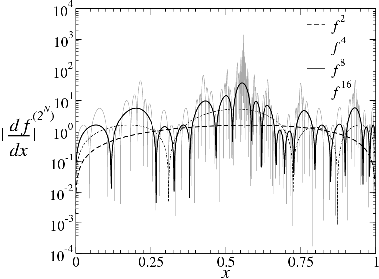
Figure 13: Absolute value of $df_{\overline{\mu}_{N}}^{(2^{N})}(x)/dx$, for ${\small N=1,2,3}$ and ${\small 4}$, on a logarithmic scale as a function of ${\small x}$ in the interval ${\small 0\leq x\leq 1}$. The proliferation of maxima conveys the development of the hierarchical structure of repellor preimages. See text.

III.1 Sequential opening of phase-space gaps

One way that the preimage structure described above is manifest in the dynamics is via the successive formation of phase-space gaps that ultimately give rise to the attractor and repellor multifractal sets. In order to observe explicitly this process we consider an ensamble of initial conditions $x_{0}$ spread out uniformly across the interval $-1\leq x_{0}\leq 1$ and keep track of their positions at subsequent times. In Figs. 14–16 we illustrate the outcome for the supercycles of periods $2^{2}$, $2^{3}$, and $2^{4}$, respectively, where we have plotted the time evolution of an ensemble composed of $10^{4}$ trajectories. In the left panel of each figure we show the absolute value of the positions $\left|x_{t}\right|$ vs time $t$, while, for comparison purposes, in the right panel we show the absolute value of $\left|x\right|$ both vs $f_{\overline{\mu}_{N}}^{(2^{N})}(x)$ and vs $\left|df_{\overline{\mu}_{N}}^{(2^{N})}/dx\right|$ to facilitate identification of the attractor and repellor positions. The labels $k=0,1,2,\ldots$ indicate the order of the gap set (or equivalently the order of the repellor generation set). In Fig. 14 (with $\mu=\overline{\mu}_{2}$) one observes a large gap opening first that contains the old repellor ($k=0$) in its middle region and two smaller gaps opening afterward that contain the two repellors of second generation ($k=1$) once more around the middle of them. In Fig. 15 (with $\mu=\overline{\mu}_{3}$) we initially observe the opening of a primary and the two secondary gaps as in the previous $\mu=\overline{\mu}_{2}$ case, but subsequently four new smaller gaps open each around the third generation of repellor positions ($k=2$). In Fig. 16 (with $\mu=\overline{\mu}_{4}$) we observe the same development as before; however, at longer times eight additional and yet smaller gaps emerge around each fourth generation of repellor positions ($k=3$). Naturally, this process continues indefinitely as $N\rightarrow\infty$ and illustrates the property mentioned before for $\mu_{\infty}$, that the time evolution at fixed control parameter values resembles progression from $\mu=0$ up to, in this section, $\overline{\mu}_{N}$. It is evident in all Figs. 14–16 that the closer the initial conditions $x_{0}$ are to the repellor positions the longer times it takes for the resultant trajectories to clear the gap regions. This intuitively evident feature is essentially linked to the knowledge we have gained about the fractal boundaries of the preimage structure, and the observable “bent over” portions of these distinct trajectories in the figures correspond to their passage across the boundaries. (Since the ensemble used in the numerical experiments is finite there appear only a few such trajectories in Figs. 14–16.)

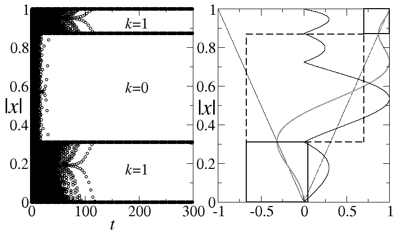
Figure 14:  Phase-space gap formation for ${\small\mu=}\overline{\mu}_{2}$. Left panel: time evolution of a uniform ensemble of $10^{4}$ trajectories as a function of $|x|$ (black areas and open circles). The values of the index ${\small k}$ label the order of the gap set. Right panel: Rotated plots of $f_{\overline{\mu}_{2}}^{(4)}(x)$(gray) and $\left|df_{\overline{\mu}_{2}}^{(4)}(x)/dx\right|$(black)  vs $|x|$ as guides for the identification of attractor and repellor positions.

To facilitate a visual comparison between the process of gap formation at $\mu_{\infty}$ and the dynamics inside the Feigenbaum attractor—as illustrated by the trajectory in Fig. 1 (right panel)—we plot in Fig. 17 the time evolution of the same ensemble composed of $10^{4}$ trajectories with $\mu=\mu_{\infty}$. This time we use logarithmic scales for both $\left|x_{t}\right|$ and $t$ and then superpose on the evolution of the ensemble the positions for the trajectory starting at $x_{0}=0$. It is clear from this figure that the larger gaps that form consecutively all have the same width in the logarithmic scale of the plot and therefore their actual widths decrease as a power law, the same power law followed, for instance, by the position sequence $x_{t}=\alpha^{-N}$, $t=2^{N}$, $N=0,1,2,\ldots$ for the trajectory inside the attractor starting at $x_{0}=0$. This set of gaps develop in time beginning with the largest one containing the $k=0$ repellor, then followed by a second gap, one of a set of two gaps associated with the $k=1$ repellor, next a third gap, one gap of a set of four gaps associated with the $k=2$ repellor, and so forth. The locations of this specific family of consecutive gaps advance monotonically towards the sparsest region of the multifractal attractor located at $x=0$. The remaining gaps formed at each stage converge, of course, to locations near other regions of the multifractal, but are not easily seen in Fig. 17 because of the specific way in which this has been plotted (and because of the scale used). In Fig. 18 we plot the same data differently, with the variable $\ln\left|x\right|$ replaced by $\ln\left|1-x\right|$, where now another specific family of gaps, one for each value of $k=0,1,2,\ldots$, appears, all with the same width on the logarithmic scale; their actual widths decrease now as $\alpha^{-2N}$, $N=0,1,2,\ldots$. The locations of this second family of consecutive gaps advance monotonically towards the most crowded region of the multifractal attractor located at $x=1$. The time necessary for the formation of successive gaps of order $k=0,1,2,\ldots$ increases as $2^{k}$ because the duration of equivalent movements of the trajectories across the corresponding preimage structures involve the $2^{k}$-th composed function $f_{\overline{\mu}_{N}}^{(2^{k})}(x)$.

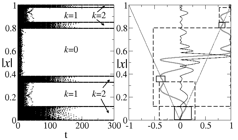
Figure 15: Phase-space gap formation for ${\small\mu=}\overline{\mu}_{3}$. Left panel: time evolution of a uniform ensemble of $10^{4}$ trajectories as a function of $|x|$ (black areas and open circles). The values of the index ${\small k}$ label the order of the gap set. Right panel: Rotated plots of $f_{\overline{\mu}_{3}}^{(8)}(x)$(gray)  and $\left|df_{\overline{\mu}_{3}}^{(8)}(x)/dx\right|$(black) vs $|x|$ as guides for the identification of attractor and repellor positions.

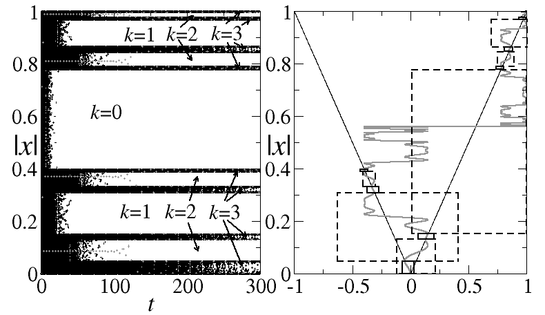
Figure 16: Phase-space gap formation for ${\small\mu=\overline{\mu}_{4}}$. Left panel: time evolution of a uniform ensemble of $10^{4}$ trajectories as a function of $|x|$ (black areas and open circles). The values of the index ${\small k}$ label the order of the gap set. Right panel: Rotated plots of $f_{\overline{\mu}_{4}}^{(16)}(x)$(gray) and $\left|df_{\overline{\mu}_{4}}^{(16)}(x)/dx\right|$(black) vs $|x|$ as guides for the identification of attractor and repellor positions.

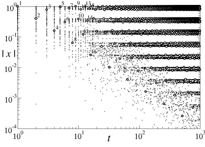
Figure 17: Phase-space gap formation for $\mu={\small\mu}_{\infty}$. The black dots correspond to time evolution of a uniform ensemble of $10^{4}$ trajectories as a function of $|x|$ vs ${\small t}$, both on logarithmic scales. The open circles are the positions, labeled by the times at which they are reached, for the trajectory inside the Feigenbaum attractor with initial condition ${\small x}_{{\small 0}}{\small=0}$, the same as the right panel in Fig. 1.

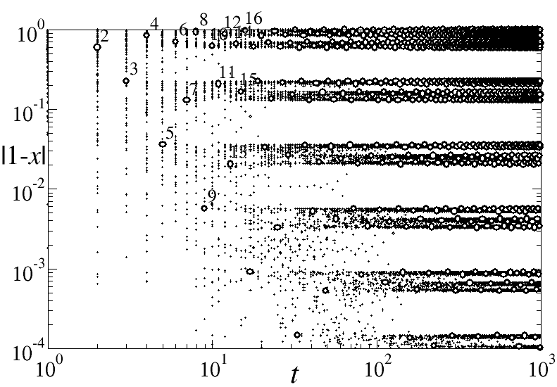
Figure 18: Same as Fig. 17 but with replacement of $|x|$ by $|{\small 1}-x|$. Notice the change in slope with respect to Fig. 17 in the opening of gaps and in the layout of the positions for the trajectory inside the attractor.

III.2 Scaling for the rates of convergence to the attractor and repellor

There is lyra1 an all-inclusive and uncomplicated way to measure the rate of convergence of an ensemble of trajectories to the attractor (and to the repellor) that consists of a single time-dependent quantity. A partition of phase-space is made of $N_{b}$ equally sized boxes or bins and a uniform distribution, of $N_{c}$ initial conditions placed along the interval $-1\leq x\leq 1$, is considered again. The number $r$ of trajectories per box is $r=N_{c}/N_{b}$. The quantity of interest is the number of boxes $W(t)$ that contain trajectories at time $t$. This is shown in Fig. 19 on logarithmic scales for the first five supercycles of periods $2^{1}$ to $2^{5}$ where we can observe the following features: In all cases $W(t)$ shows a similar initial nearly constant plateau [$W(t)\simeq\Delta$, $1\leq t_{1}\leq t_{0}$, $t_{0}=O(1)$] and a final well-defined decay to zero. As it can be observed in the left panel of Fig. 19 the duration of the final decay grows (approximately) proportionally to the period $2^{N}$ of the supercycle. There is an intermediate slow decay of $W(t)$ that develops as $N$ increases with duration also (just about) proportional to $2^{N}$. For the shortest period $2^{1}$, there is no intermediate feature in $W(t)$; this appears first for period $2^{2}$ as a single dip and expands with one undulation every time $N$ increases by one unit. The expanding intermediate regime exhibits the development of a power law decay with the logarithmic oscillations characteristic of discrete scale invariance sornette1 . Clearly, the manifestation of discrete invariance is expected to be associated with the period-doubling cascade. In the right panel of Fig. 19 we show a superposition of the five curves in Fig. 19 (left panel) obtained via rescaling of both $W(t)$ and $t$ for each curve according to repeated scale factors.

The limiting form $W(t)$ for $N\rightarrow\infty$ is shown in the left panel of Fig. 20 for various values of $r$ while in its right panel we show, for $r=100$, a scale amplification of $W(t)$ with the same factors employed in Fig. 19 for the supercycles with small periods. The behavior of $W(t)$ at $\mu_{\infty}$ was originally presented in Ref. lyra1 , where the power law exponent $\varphi$ and the logarithmic oscillation parameter $\Lambda$ in

$$W(t)\simeq\Delta h\left(\frac{\ln\tau}{\ln\Lambda}\right)\tau^{-\varphi},\;\tau=t-t_{0},$$ (2)

were obtained numerically with a precision that corresponds to $r=10$. In Eq. (2) $h(x)$ is a periodic function with $h(1)=1$ and $\Lambda$ is the scaling factor between the periods of two consecutive oscillations. More recently, in Ref. grassberger1 , it was pointed out that numerical estimates of $W(t)$ are subject to large finite-size corrections, and, also, that $W(t)$ should scale with the intervals in the triadic cantor set construction of the Feigenbaum attractor grassberger1 , from which the value for $\varphi\cong 0.800138194$ is reported. The values for the rescaling factors in our Figs. 19 and 20 suffer from these large finite-size effects due to the relatively small values of $r$ used in the calculations. This is evident since the time scaling factor obtained from these data differs by $10\%$ from the exact value of $\Lambda=2$ implied by the discrete scale invariance property created by the period-doubling cascade. In Fig. 21 we show the rate $W(t)$ and the superposition of repeated amplifications of itself (as in the right panel of Fig. 20) for increasing values of $N_{c}$. We find that the scaling factor $\Lambda$ converges to its limit $\Lambda=2$.

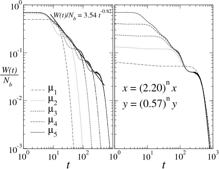
Figure 19: Left panel: Rate ${\small W(t)}$, divided by the number of boxes ${\small N}_{b}$ employed, of approach to the attractor for the supercycles of periods ${\small 2}^{{\small N}}$, ${\small N=1,2,3,4}$ and ${\small 5}$ on logarithmic scales. The expression shown corresponds to the power-law decay of the developing logarithmic oscillations. Right panel: Superposition of the five curves for ${\small W(t)}$ in the left panel via ${\small n}$-times repeated rescaling factors shown for the horizontal ${\small x}$ and vertical ${\small y}$ axes.

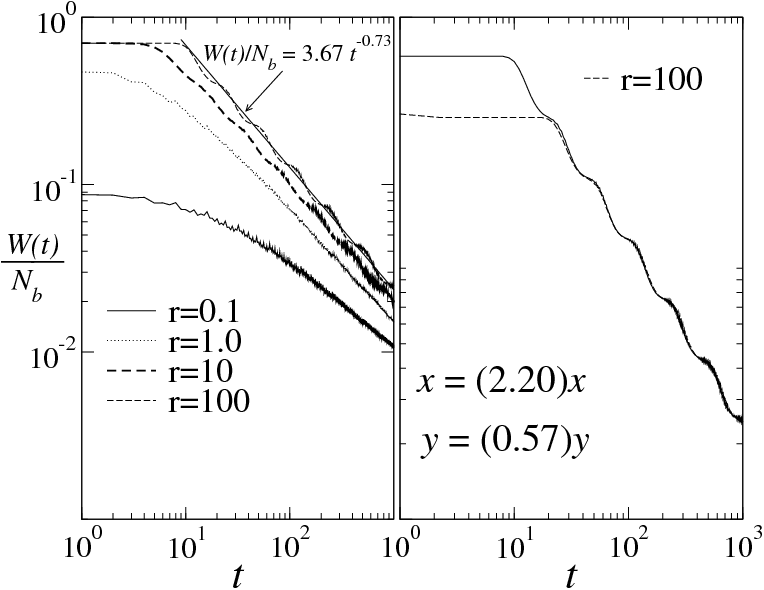
Figure 20: Left panel: Rate ${\small W(t)}$ of approach to the Feigenbaum attractor at $\mu={\small\mu}_{\infty}$ on logarithmic scales. The curves correspond to the values given for the number ${\small r}$ of trajectories per box, and the expression shown corresponds to power law decay with logarithmic oscillations. Right panel: Superposition of ${\small W(t)}$, for ${\small r=100}$, on itself via the rescaling shown (the same as in Fig. 19) for the horizontal ${\small x}$ and vertical ${\small y}$ axes.

We are now in a position to appreciate the dynamical mechanism at work behind the features of the decay rate $W(t)$. From our previous discussion we know that, every time the period of a supercycle increases from $2^{N-1}$ to $2^{N}$ by a shift the control parameter value from $\overline{\mu}_{N-1}$ to $\overline{\mu}_{N}$, the preimage structure advances one stage of complication in its hierarchy. Along with this, and in relation to the time evolution of the ensemble of trajectories, an additional set of $2^{N}$ smaller phase-space gaps develops and also a further oscillation takes place in the corresponding rate $W(t)$ for finite-period attractors. At $\mu=\mu_{\infty}$ the time evolution tracks the period-doubling cascade progression, and every time $t$ increases from $2^{N-1}$ to $2^{N}$ the flow of trajectories undergoes equivalent passages across stages in the itinerary through the preimage ladder structure, in the development of phase-space gaps, and in logarithmic oscillations in $W(t)$. In Fig. 22 we show the correspondence between these features quantitatively.

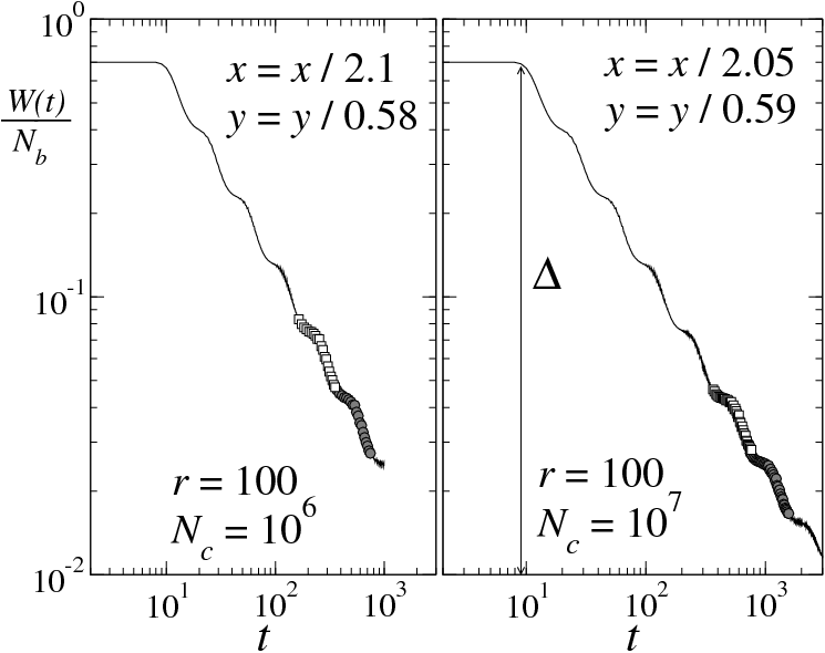
Figure 21: Same as in the right panel of Fig. 20 but obtained with increased precision. In the left panel the number of initial conditions is ${\small N}_{c}{\small=10}^{6}$, while in the right panel ${\small N}_{c}{\small=10}^{7}$. The distance $\Delta$ is $\Delta=(1+|-1/\alpha|)/(1+|-1|)$, where $\alpha$ is Feigenbaum’s constant. This stems from the fact that all initial conditions out of the interval $(-1/\alpha,1)$ take a value inside this interval in the first iteration. As can be observed, the scaling factor for the horizontal axis converges to the exact value ${\small x=2}$.

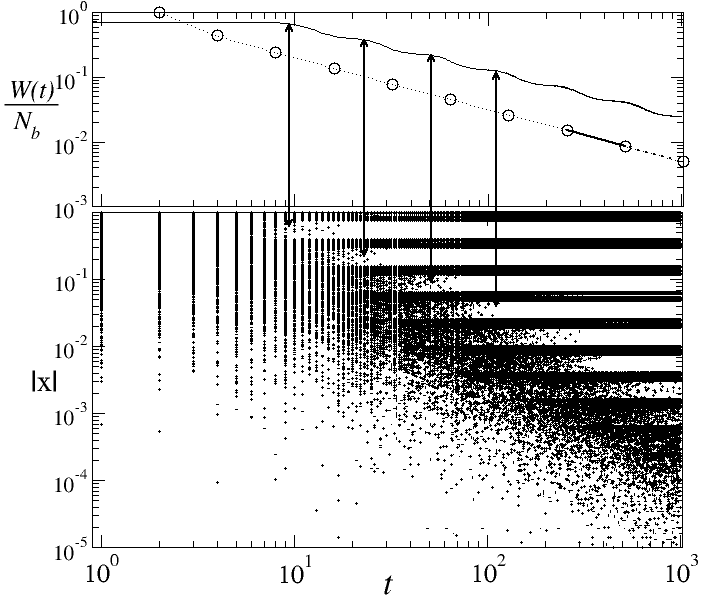
Figure 22: Correspondence between the power law decay with log-periodic oscillation features of the rate ${\small W(t)}$ with the sequential opening of phase-space gaps. Top panel: The solid line is ${\small W(t)}$ from Fig. 21 and the open circles values are obtained for ${\small W(t)}$ from Eq. (3) at times $t={\small 2}^{{\small N}}$, $N=1,2,\ldots$ See text.

IV $q$-deformed statistical-mechanical structure

The rate $W(t)$, at the values of time for period doubling, can be obtained quantitatively from the supercycle diameters $d_{N,m}$. Specifically, $W(t)=\Delta\ Z_{\tau}$, $\Delta=(1+\alpha^{-1})/2$ note2 , $\tau=t-t_{0}$, and

$$Z_{\tau}=\sum_{m=0}^{2^{N-1}-1}d_{N,m},\;\tau=2^{N-1},\;N=1,2,3,...$$ (3)

Eq. (3) is an explicit expression equivalent to the numerical procedure followed in Ref. grassberger1 by the use of the triadic cantor set construction of the Feigenbaum attractor to evaluate the power law exponent $\varphi$, and from which the value for $\varphi\cong 0.800138194$ is reported. In Fig. 22 we have added the results of a calculation of $W(t)$ at times $\tau=2^{N}$, $N=1,2,\ldots$, according to Eq. (3).

The predicted statistical-mechanical structure is exposed when we identify the (scaled and shifted) decay rate $Z_{\tau}$ as a partition function. From this viewpoint the diameters $d_{N,m}$ are configurational terms that in a true statistical-mechanical theory would be expected to obey some well-defined statistical weights, such as Boltzmann factors. To check on this we proceed to determine their time dependence given by the bifurcation index $N$. The $d_{N,m}$ scale (asymptotically) with $N$ for $m/2^{N}$ fixed as

$$d_{N,m}\simeq\alpha_{y}^{-N+1},\;N\;large$$ (4)

where the $\alpha_{y}$ are universal constants obtained, for instance, from the finite jump discontinuities of Feigenbaum’s trajectory scaling function $\sigma(y)=\lim_{n\rightarrow\infty}d_{N,m+1}/d_{N,m}$, $y=\lim_{N\rightarrow\infty}m/2^{N}$ schuster1 . The two largest discontinuities of $\sigma(y)$ correspond to the thinner and the fuller regions of the multifractal attractor, and for these two regions we have, respectively, $d_{N,0}\simeq\alpha^{-N+1}$ and $d_{N,1}\simeq\alpha^{-2(N-1)}$. [The length of the first diameter is $d_{1,0}=1$ and the equality in Eq. (4) is approached rapidly with increasing $N$.] The power law in Eq. (4) can be rewritten as a $q$-exponential ($\exp_{q}(x)\equiv[1-(q-1)x]^{-1/(q-1)}$) via use of the identity $A^{-N+1}\equiv(1+\beta)^{-\ln A/\ln 2}$, $\beta=2^{N-1}-1$, that is,

$$d_{N,m}\simeq\exp_{q_{y}}(-\beta\nu_{y}),$$ (5)

where $q_{y}=1+\nu_{y}^{-1}$, $\nu_{y}=\ln\alpha_{y}/\ln 2$, and $\beta=\tau-1=2^{N-1}-1$. Similarly, the partition function $Z_{\tau}\simeq\tau^{-\varphi}$ (or $Z_{\tau}\simeq\varepsilon^{-N+1}$), with $\varphi=\ln\varepsilon/\ln 2$ and $\tau=2^{N-1}$, can be expressed as

$$Z_{\tau}\simeq\exp_{Q}(-\beta\varphi),$$ (6)

where $Q=1+\varphi^{-1}$ and once more $\beta=\tau-1=2^{N-1}-1$.

Our main contention becomes evident when Eqs. (5) and (6) are used in Eq. (3), to yield

$$\exp_{Q}(-\beta\varphi)\simeq\sum_{y}\exp_{q_{y}}(-\beta\nu_{y}).$$ (7)

Eq. (7) is similar to a basic statistical-mechanical expression; the quantities in it take the following parts: $\beta$ an inverse temperature, $\varphi$ a free energy (or the product $s=-\beta\varphi$ a Massieu thermodynamic potential, or entropy), and the $\nu_{y}$ configurational energies. However, the equality involves $q$-deformed exponentials in place of ordinary exponential functions that would be recovered when $Q=q_{m}=1$. It is worth noticing that there is a multiplicity of $q$-indices associated to the configurational weights in Eq. (7); however, their values form a well-defined family robledo3 determined by the discontinuities of Feigenbaum’s function $\sigma$.

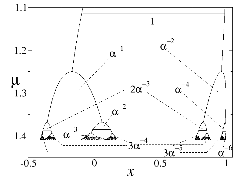
Figure 23: Sector of the bifurcation tree for the logistic map ${\small f}_{\mu}{\small(x)}$ that shows the formation of a Pascal triangle of diameter lengths according to the scaling approximation explained in the text, where ${\small\alpha\simeq 2.5091}$ is the pertinent universal constant.

In the spirit of a mean field approximation we suppose that, for a given value of $N$, e.g., $N=3$, the diameters $d_{N,m}$ that are of similar lengths have actually equal length, and this length is obtained from those of the shortest or longest diameters via a simple scale factor; e.g., $d_{3,3}=d_{3,2}=$ $\alpha^{-1}d_{3,0}=$ $\alpha d_{3,1}$. This initiates a degree of degeneracy in the lengths that subsequently spreads all the way through the bifurcation tree. See Fig. 23 linage1 . As a result of this approximation, the $d_{N,m}$ scale with increasing $N$ according to a binomial combination of the scale factors of those diameters that converge to the most crowded and most sparse regions of the multifractal attractor. To be precise, the $2^{N-1}$ diameters at the $N$-th supercycle have lengths equal to $\alpha^{-(N-1-l)}\alpha^{-2k}$ and occur with multiplicities ${N-1\choose k}$, where $k=0,1,...,N-1$. As shown in Fig. 23 the diameters create a Pascal triangle across the bifurcation cascade. This feature greatly simplifies the evaluation of the partition function and directly yields

$$Z_{\tau}=\sum_{k=0}^{N-1}{N-1\choose k}\alpha^{-(N-1-k)}\alpha^{-2k}=\left(\alpha^{-1}+\alpha^{-2}\right)^{N-1},$$ (8)

$\tau=2^{N-1}$. We obtain $\varepsilon=\left(\alpha^{-2}+\alpha^{-1}\right)=1.7883$, $\varphi=0.8386$, and $Q=2.1924$, a surprisingly good approximation when compared to the numerical estimates $\varphi=0.8001$and $Q=2.2498$ of the exact values. Under this approximation all the indices $q_{y}$ in Eq. (7) are equal, $q_{y}=q=1+\nu^{-1}$, $\nu=\ln\alpha/\ln 2$, and Eq. (7) becomes

$$\exp_{Q}(-\beta\varphi)=\sum_{k=0}^{N-1}\Omega(N-1,k)\exp_{q}(-\beta\nu),$$ (9)

where $\Omega(N-1,k)=\alpha^{-l}$ ${N-1\choose k}$. In thermodynamic language, the approach to the attractor described by Eq. (7) or (9) is a cooling process $\beta\rightarrow\infty$ in which the free energy (or energy) $\varphi$ is fixed and therefore the entropy $s=-\beta\varphi$ is linear in $\beta$. It is instructive to define an “energy landscape” for the Feigenbaum attractor as being composed of an infinite number of “valleys” whose equal-valued minima at $\beta\rightarrow\infty$ coincide with the points of the attractor on the interval $[-\alpha^{-1},1]$ note2 . When $\beta=2^{N-1}-1$, $N$ finite, the valleys merge into $2^{N-1}$ intervals of widths equal to the diameters $d_{N,m}$.

As established some time ago, the so-called thermodynamic formalism beck1 is built around the statistical-mechanical framework followed by the geometric properties of multifractals. The partition function formulated to study their properties, like the spectrum of singularities $f(\widetilde{\alpha})$ beck1 , is

$$Z(\widetilde{\mathsf{\tau}},\mathsf{q})\equiv\sum_{m}^{M}p_{m}^{\widetilde{\mathsf{\tau}}}l_{m}^{-\mathsf{q}},$$ (10)

where the $l_{m}$ (in one-dimensional systems) are $M$ disjoint interval lengths that cover the multifractal set and the $p_{m}$ are probabilities given to these intervals. The standard practice consists of demanding that $Z(\mathsf{\tau},\mathsf{q})$ neither vanishes nor diverges in the limit $l_{m}\rightarrow 0$ for all $m$ (and consequently $M\rightarrow\infty$). Under this condition the exponents $\widetilde{\mathsf{\tau}}$ and $\mathsf{q}$ define a function $\widetilde{\mathsf{\tau}}(\mathsf{q})$ from which $f(\widetilde{\alpha})$ is obtained via Legendre transformation beck1 . When the multifractal is an attractor its elements are ordered dynamically, and for the Feigenbaum attractor the trajectory with initial condition $x_{0}=0$ generates in succession the positions that form the diameters, generating all diameters $d_{N,m}$ for $N$ fixed between times $\tau=2^{N-1}$ and $\tau=3\times 2^{N-1}$. Because the diameters cover the attractor it is natural to choose the covering lengths at stage $N$ to be $l_{m}^{(N)}=$ $d_{N,m}$ and to assign to each of them the same probability $p_{m}^{(N)}=1/2$. For example, within the two-scale approximation to the Feigenbaum multifractal beck1 , $l_{k}^{(N)}=\alpha^{-(N-1-k)}\alpha^{-2k}$, the condition $Z(\widetilde{\mathsf{\tau}},\mathsf{q})=1$ reproduces Eq. (8) when $p_{m}^{(N)}=$ $\tau^{-1}=2^{-N+1}$, with $\widetilde{\mathsf{\tau}}=1$ and $\mathsf{q}=-\varphi$. It should be kept in mind that the “static” partition function $Z(\widetilde{\mathsf{\tau}},\mathsf{q})$ is not meant to distinguish between chaotic and critical (vanishing $\lambda$) multifractal attractors as we do here. As we emphasize below, it is the functional form of the link between the probabilities $p_{m}^{(N)}$ and actual time $\tau$ that determines the nature of the statistical mechanical structure of the dynamical system.

A crossover to $q=1$ ordinary statistics when a critical attractor turns chaotic; this can be explained as follows. We first recall that multifractal sets and their statistical-mechanical properties can be retrieved by means of the recursive method of backward iteration of chaotic maps mccauley1 . A chaotic unimodal map has a two-valued inverse and given a position $x=x_{n}$ a binary tree is formed under backward iteration, so there are $2^{n}$ initial conditions $x_{0}$ for trajectories that lead to $x_{n}$. Since in this case the Lyapunov exponent is positive $\lambda>0$, lengths expand under forward iteration according to $l\sim\exp(\lambda n)$ and contract under backward iteration as $l\sim\exp(-\lambda n)$. We can define, as above, a set of covering lengths $D_{n,m}=$ $\Delta_{m}\exp(-\lambda n)$, where $m$ relates to the initial condition $x_{0}$ and use of them in a partition function like that in Eq. (3) gives

$$\exp(-\beta\varphi)=\sum_{m}\Delta_{m}\exp(-\beta\lambda),$$ (11)

where now $\beta=n$. Keeping in mind Pesin’s theorem $\varphi$ is plainly identified as the Kolmogorov-Sinai entropy. Now, the crossover from $q$-deformed statistics to ordinary $q=1$ statistics can be observed for control parameter values in the vicinity of the Feigenbaum attractor, $\mu\gtrsim\mu_{\infty}$, when the attractor consists of $2^{\overline{n}}$ bands, $\overline{n}$ large. The Lyapunov coefficient $\lambda$ of the chaotic attractor decreases with $\Delta\mu=\mu-$ $\mu_{\infty}$ as $\lambda\varpropto 2^{-\overline{n}}\sim\Delta\mu^{\kappa}$, $\kappa=\ln 2/\ln\delta_{F}$, where $\delta_{F}$ is the Feigenbaum constant that measures the rate of development of the bifurcation tree in control parameter space schuster1 . The chaotic orbit consists of an interband periodic motion of period $2^{\overline{n}}$ and an intraband chaotic motion. The expansion rate $\sum_{i=0}^{\tau-1}\ln\left|df_{\mu}(x_{i})/dx_{i}\right|$ fluctuates with increasing amplitude as $\ln\tau$ for $\tau<2^{\overline{n}}$ but converges to a fixed number that grows linearly with $\tau$ for $\tau\gg 2^{\overline{n}}$ mori1 . This translates as dynamics with $q\neq 1$ for $\tau<2^{\overline{n}}$ but ordinary dynamics with $q=1$ for $\tau\gg 2^{\overline{n}}$.

V Summary

As stated, the dynamics of critical attractors in low-dimensional nonlinear maps is a suitable phenomenon for assessing the limits of validity and generalizations of ordinary statistical mechanics. There are now positive indications that the multifractal critical attractors present in these maps play this role, since, as it turns out, the two sets of dynamical properties— inside and towards the Feigenbaum attractor—appear combined in a $q$-deformed statistical-mechanical structure robledo00 . To obtain this remarkable property it is necessary to have access to detailed information for these two different types of properties. The dynamics at the attractor (for both trajectories and sensitivity to initial conditions) has been analyzed in detail before for period doubling robledo2 ; robledo3 and for the quasiperiodic robledo7 transition to chaos. But the dynamics on the way to the attractor is only now offered as far as we know.

To begin with, we studied the properties of the first few members of the family of superstable attractors of unimodal maps with quadratic maxima and obtained a precise understanding of the complex labyrinthine dynamics that develops as their period $2^{N}$ increases. The study is based on the determination of the function $t_{f}(x_{0})$, the time of flight for a trajectory with initial condition $x_{0}$ to reach the attractor or repellor. The function $t_{f}(x_{0})$ was determined for all initial conditions $x_{0}$ in a partition of the total phase-space $-1\leq x_{0}\leq 1$, and this provides a complete picture for each attractor-repellor pair. We observed how the fractal features of the boundaries between the basins of attraction of the positions of the periodic orbits develop a structure with hierarchy, and how this in turn reflects on the properties of the trajectories. The set of trajectories produces an ordered flow towards the attractor or towards the repellor that reflects the ladder structure of the sub-basins that constitute the mentioned boundaries. As $2^{N}$ increases there is sensitivity to the final position for almost all $x_{0}$, and there is a transient exponentially-increasing sensitivity to initial conditions for almost all $x_{0}$. We observed that transient chaos is the manifestation of the trajectories’ controlled flow out of the fractal boundaries, which suggests that for large $2^{N}$ the flow becomes an approximately self-similar sequence of stages. As a final point, in the Appendix, we look at the closing segment of trajectories at which a very fast convergence to the attractor positions occurs. We found “universality class” features, as the trajectories and sensitivity to initial conditions are replicated by a RG fixed-point map obtained under functional composition and rescaling. This map has the same $q$-deformed exponential closed form found to hold also for the pitchfork and tangent bifurcations of unimodal maps robledo5 ; robledo6 .

Subsequently, we examined the process followed by an ensemble of uniformly distributed initial conditions $x_{0}$ across the phase-space to arrive at the Feigenbaum attractor, or get captured by its corresponding repellor. Significantly, we gained understanding concerning the dynamical ordering in $x_{0}$, in relation to the construction of the families of phase-space gaps that support the attractor and repellor, and about the rate of approach of trajectories towards these multifractal sets, as measured by the fraction of bins $W(t)$ still occupied by trajectories at time $t$. An important factor in obtaining this knowledge has been the consideration of the equivalent dynamical properties for the supercycles of small periods in the bifurcation cascade. As we have seen, a doubling of the period introduces well-defined additional elements in the hierarchy of the preimage structure, in the family of phase-space gaps, and in the log-periodic power law decay of the rate $W(t)$. We have then corroborated the wide-ranging correlation between time evolution at $\mu_{\infty}$ from $t=0$ up to $t\rightarrow\infty$ with the static period-doubling cascade progression from $\mu=0$ up to $\mu_{\infty}$. As a result of this we have acquired an objective insight into the complex dynamical phenomena that fix the decay rate $W(t)$. We have clarified the genuine mechanism by means of which the discrete scale invariance implied by the log-periodic property in $W(t)$ arises, that is, we have seen how its self-similarity originates in the infinite hierarchy formed by the preimage structure of the attractor and repellor. The rate $W(t)$ can be obtained quantitatively [see Eq. (3)] from the supercycle diameters $d_{N,m}$. These basic data descriptive of the period-doubling route to chaos are also a sufficient ingredient in the determination of the anomalous sensitivity to initial conditions for the dynamics inside the Feigenbaum attractor robledo3 .

Finally, the case is made that there is a statistical-mechanical property underlying the dynamics of an ensemble of trajectories en route to the Feigenbaum attractor (and repellor). Eq. (3) is identified as a partition function built of $q$-exponential weighted configurations, and in turn, the fraction $Z_{\tau}$ of phase-space still occupied at time $\tau$ is seen to have the form of the $q$-exponential of a thermodynamic potential function. This is argued to be a concrete, clear and genuine manifestation of $q$-deformation of ordinary statistical mechanics where arguments can be made explicit and rigorous. There is a close resemblance with the thermodynamic formalism for multifractal sets, but it should be stressed that the deviation from the usual exponential statistics is dynamical in origin, and due to the vanishing of the (only) Lyapunov exponent.

Acknowledgments. We are grateful to Dan Silva for useful preliminary studies, to Jorge Velazquez Castro for valuable help and to Hugo Hernández Saldaña for interesting discussions. Partial support by DGAPA-UNAM and CONACyT (Mexican agencies) as well as SIMUMAT (Comunidad de Madrid, Spanish agency) is acknowledged.

VI Appendix: Super-strong insensitivity to initial conditions

The ordinary Lyapunov exponent $\lambda\equiv\lim_{t\rightarrow\infty}t^{-1}\ln\left.df_{\overline{\mu}_{N}}^{(t)}(x)/dx\right|_{x=0}$ for the supercycle attractors diverges to minus infinity [$df_{\overline{\mu}_{N}}^{(t)}(x)/dx=0$ at $x=0$], therefore the sensitivity to initial conditions $\xi_{t}$ cannot have an exponential form $\xi_{t}=\exp(\lambda t)$ with $\lambda<0$. This appendix is a brief account of the determination of $\xi_{t}$ at the closing point of approach to the supercycle attractors.

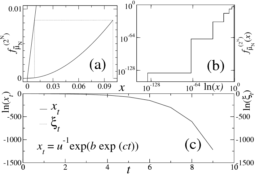
Figure 24: Panel (a): Detail of a trajectory in its final stage of approach to the ${\small x=0}$ attractor position (dotted line) for the map $f_{\overline{\mu}_{N}}^{(2^{N})}(x)$ (solid line). In this example ${\small N=3}$. Panel (b): Same as (a) in double logarithmic scale. Panel (c): Trajectory $x_{t}$ and sensitivity to initial conditions $\xi_{t}$ in logarithmic scale versus time ${\small t}$. Both functions are indistinguishable. Note that there is an ultra-rapid convergence, of only a few time steps, to the origin ${\small x=0}$. See text.

Representative results for the last segment of a trajectory and the corresponding sensitivity $\xi_{t}$ obtained from a numerical investigation are shown in Fig. 24. Only the first two steps of a trajectory with $x_{0}=0.1$ of the map $f_{\overline{\mu}_{3}}^{(2^{3})}$ can be seen in Fig. 24(a). A considerable enlargement of the spatial scale (which requires computations of extreme precision mapm1 ) makes it possible to observe a total of seven steps ($56$ iterations in the original map), as shown with the help of logarithmic scales in Fig. 24(b). Fig. 24(c) shows both the same trajectory and the sensitivity $\xi_{t}\equiv dx_{t}/dx_{0}$ in a logarithmic scale for $x_{t}$ and $\xi_{t}$ and a normal scale for the time $t$. The trajectory is accurately reproduced [indistinguishable from the curve in Fig. 24 (c)] by the expression $x_{t}=u^{-1}\exp(b\exp ct)$, $b=\ln ux_{0}$ (with $x_{0}>0$), and $c=\ln 2$, where $u>0$ is obtained from the form $|f_{\overline{\mu}_{N}}^{(2^{N})}|\simeq ux^{2}$ taken by the $2^{N}$-th composed map close to $x=0$. This expression for $x_{t}$ is just another form of writing $ux_{t}=(ux_{0})^{2^{t}}$, the result of repeated iteration of $ux^{2}$. For the logarithm of the sensitivity we have $\ln\xi_{t}=-\ln x_{0}+t\ln 2+\ln x_{t}$ where the last (large negative) term dominates the first two. Thus, we find that the sensitivity decreases more quickly than an exponential, and, more precisely, decreases as the exponential of an exponential.

We note that, associated with the general form $f_{\overline{\mu}_{N}}^{(2^{N})}(x)\simeq ux^{2}$ of the map in the neighborhood of $x=0$, there is a map $f^{\ast}(x)$ that satisfies the functional composition and rescaling equation $f^{\ast}(f^{\ast}(x))=a^{-1}f^{\ast}(ax)$ for some finite value of $a$ and such that $f^{\ast}(x)=ux^{2}+o(x^{4})$. The fixed-point map $f^{\ast}(x)$ possesses properties common to all superstable attractors of unimodal maps with a quadratic extremum. Indeed, there is a closed form expression that satisfies these conditions, which is $f^{\ast}(x)=x\exp_{q}(u^{q-1}x).$ The fixed-point map equation is satisfied with $a=2^{1/(q-1)}$ and $q=1/2$. The same type of RG solution has been previously found to exist for the tangent and pitchfork bifurcations of unimodal maps with general nonlinearity $z>1$ hu1 ; robledo5 ; robledo6 . Use of the map $f^{\ast}(x)$ reproduces the trajectory $x_{t}/x_{0}$ and sensitivity $\xi_{t}$ shown in Fig. 24 (c).

References

- (1) See, for example, C. Beck, F. Schlogl, Thermodynamics of Chaotic Systems, Cambridge University Press, UK, 1993.
- (2) H. Mori, H. Hata, T. Horita and T. Kobayashi, Prog. Theor. Phys. Suppl. 99, 1 (1989).
- (3) See A. Robledo, Europhys. News 36, 214 (2005), and references therein.
- (4) E. Mayoral, A. Robledo, Phys. Rev. E 72, 026209 (2005).
- (5) G. Anania and A. Politi, Europhys. Lett. 7, 119 (1988).
- (6) T.C. Halsey, M.H. Jensen, L.P. Kadanoff, I. Procaccia, B.I. Shraiman, Phys. Rev. A 33, 1141 (1986).
- (7) J.-P. Eckmann and I. Procaccia, Phys. Rev. A 34, 659 (1986).
- (8) M. Sano, S. Sato and Y. Yawada, Prog. Theor. Phys. 76, 945 (1986).
- (9) Here we use the term -deformed statistical mechanics with reference to the occurrence of statistical-mechanical expressions where instead of the ordinary exponential and logarithmic functions appear their -deformed counterparts. The -deformed exponential function is defined as , and its inverse, the -deformed logarithmic function as . The ordinary exponential and logarithmic functions are recovered when .
- (10) A. Robledo, Physica A 370, 449 (2006).
- (11) C. Tsallis, J. Stat. Phys. 52, 479 (1988).
- (12) A brief account of some of the main conclusions drawn here is given in A. Robledo, arXiv:0710.1047 [cond-mat.stat-mech], additional related material appears in Robledo A., Moyano, L.G., “Some aspects of the dynamics towards supercycle attractors and their accumulation point, the Feigenbaum attractor”, in Complexity, Metastability and Nonextensivity-CTNEXT 07, edited by S. Abe, H. Herrmann, P. Quarati, A. Rapisarda, and C. Tsallis, American Institute of Physics (2007), pp. 114-121.
- (13) F. Baldovin and A. Robledo, Phys. Rev. E 72, 066213 (2005).
- (14) F.A.B.F. de Moura, U. Tirnakli and M.L. Lyra, Phys. Rev. E 62, 6361 (2000).
- (15) H.G. Schuster, Deterministic Chaos. An Introduction, 2nd revised ed. (VCH, Weinheim, 1988).
- (16) A. Robledo, Physica A 314, 437 (2002); Physica D 193, 153 (2004).
- (17) F. Baldovin, A. Robledo, Europhys. Lett. 60, 518 (2002).
- (18) B. Hu and J. Rudnick, Phys. Rev. Lett. 48, 1645 (1982).
- (19) C. Grebogi, S.W. McDonald, E. Ott, J.A. Yorke, Phys. Lett. 99A, 415 (1983).
- (20) S.W. McDonald, C. Grebogi, E. Ott, J.A. Yorke, Physica 17D, 125 (1985).
- (21) D. Sornette, Phys. Rep. 297, 239 (1998).
- (22) P. Grassberger, Phys. Rev. Lett. 95, 140601 (2005).
- (23) See caption of Fig. 21.
- (24) G. Linage, F. Montoya, A. Sarmiento, K. Showalter, P. Parmananda, Phys. Lett. A 359, 638 (2006).
- (25) J.L. McCauley, Int. J. Mod. Phys. B3, 821 (1989).
- (26) H. Hernández-Saldaña, A. Robledo, Physica A 370, 286 (2006).
- (27) Our simulations used MAPM, the arbitrary precision C++ library (http://www.tc.umn.edu/ ringx004/mapm-main.html). We implemented our calculations taking between 200 and 1200 significant digits.