1 Introduction

The cancellation of gauge anomalies in the Standard Model (SM) is a landmark of modern particle theory that has contributed to shape our knowledge on the fermion spectrum, its chiral charges and couplings. Other mechanisms of cancellation, based on the introduction of both local and non-local counterterms, have also received a lot of attention in the last two decades, from the introduction of the Wess-Zumino term in gauge theories [1] (which is local) to the Green-Schwarz mechanism of string theory [2] (which is non-local). The field theory realization of this second mechanism is rather puzzling also on phenomenological grounds since it requires, in four dimensions, the non-local exchange of a pseudoscalar to restore gauge invariance in the anomalous vertices. In higher dimensions, for instance in 10 dimensions, the violation of the Ward identities due to the hexagon diagram is canceled by the exchange of a 2-form [2, 3]. In this work we are going to analyze the similarities between the two approaches and emphasize the differences as well. We will try, along the way, to point out those unclear aspects of the field theory realization of this mechanism - in the absence of supersymmetry and gravitational interactions - which, apparently, suffers from the presence of an analytic structure in the energy plane that is in apparent disagreement with unitarity. Moving to the WZ case, here we show that the restoration of gauge invariance in the corresponding one-loop effective Lagrangian via a local axion counterterm is not able to guarantee unitarity beyond a certain scale, although this deficiency is expected [4, 5], given the local nature of the counterterm. In the GS case, the restoration of the Ward identities suffers from the presence of unphysical massless poles in the trilinear gauge vertices that, as we are going to show, are similar to those present in a non-local version of axial electrodynamics, which has been studied extensively in the past [6] with negative conclusions concerning its unitarity properties. In particular, in the case of scalar potentials that include Higgs- axion mixing, the phenomenological interpretation of the GS mechanism remains problematic in the field theoretical construction.

We comment on the relation between the two mechanisms, when the axion is integrated out of the partition function of the anomalous theory, and on other issues of the gauge dependence of the perturbative expansions, which emerge in the different formulations. In the second part of this work we apply our analysis to a realistic model characterizing numerically the bounds in effective actions of WZ type and discuss the possibility to constrain brane and axion-like models at the LHC.

1.1 WZ and GS counterterms

Anomalous abelian models are variations of the standard model in which the gauge structure of this is enlarged by one or more abelian factors. The corresponding anomalies are canceled by the introduction of a pseudoscalar, an axion ($b$), that couples to 4-forms $F_{I}\wedge F_{J}$ (via $b/MF_{I}\wedge F_{J}$, the Wess-Zumino term) of the gauge fields $(I,J)$ that appear both in ordinary $(I=J)$ and mixed $(I\neq J)$ anomalies. $M$ is a scale that is apparently unrelated to the rest of the theory and simply describes the range in which the anomalous model can be used as a good approximation to the underlying complete theory. The latter can be resolved at an energy $E>M$, by using either a renormalizable Lagrangian with an anomaly-free chiral fermion spectrum or a string theory. The motivations for introducing such models are several, ranging from the study of the flavor sector, where several attempts have been performed in the last decade to reproduce the neutrino mixing matrix using theories of this type, to effective string models, in which the extra $U(1)$ abound. We also recall that in effective string models and in models characterized by extra dimensions the axion ($b$) appears together with a mixing to the anomalous gauge boson ($\partial{b}B$), which is, by coincidence, natural in a (Higgs) theory in a broken phase. In a way, theories of this type have several completions at higher energy [5].

Coming to the specific models that we analyze, these are complete MLSOM-like [7, 8] models with three anomalous $U(1)$ [9, 10], while most of the unitarity issues are easier to address in simple models with two U(1) [11]. In our phenomenological analysis, which concerns only effective actions of WZ type, we will choose the charge assignments and the construction of [12], but we will work in the region of parameter space where only the lowest Stückelberg mass eigenvalue is taken into account, while the remaining two extra $Z^{\prime}$ decouple. This configuration is not the most general but is enough to clarify the key physical properties of these models.

2 Anomaly cancellation and gauge dependences: the GS and the WZ mechanisms in field theory

In this section we start our discussion of the unitarity properties of the GS and WZ mechanisms, illustrating the critical issues. We illustrate a pure diagrammatic construction of the WZ effective action using a set of basic local counterterms and show how a certain class of amplitudes have an anomalous behavior that grows beyond their unitarity limit at high energy. The arguments being rather subtle, we have decided to illustrate the construction of the effective action for both mechanisms in parallel. A re-arrangement of the same basic counterterms of the WZ case generates the GS effective action, which, however, is non-local. The two mechanisms are different even if they share a common origin. In a following section we will integrate out the axion of the WZ formulation to generate a non-local form of the same mechanism that resembles more closely the GS counterterm. The two differ by a set of extra non-local interactions in their respective effective actions. One could go the other way and formulate the GS mechanism in a local form using (two or more) extra auxiliary fields. These points are relevant in order to understand the connection between the two ways to cancel the anomaly.

2.1 The Lagrangian

Specifically, the toy model that we consider has a single fermion with a vector-like interaction with the gauge field $A$ and a purely axial-vector interaction with $B$. The Lagrangian is given by

$$\mathcal{L}_{0} = -\frac{1}{4}F_{A}^{2}-\frac{1}{4}F_{B}^{2}+\frac{1}{2}(\partial_{\mu}b+M_{1}\ B_{\mu})^{2}+\overline{\psi}i\gamma^{\mu}(\partial_{\mu}+ieA_{\mu}+ig_{B}\gamma^{5}B_{\mu})\psi,$$ (1)

where, for simplicity, we have taken all the charges to be unitary, and we have allowed for a Stückelberg term for $B$, with $M_{1}$ being the Stückelberg mass . $A$ is massless and takes the role of a photon. The Lagrangian has a Stückelberg-like symmetry with $b\to b-M_{1}\theta_{B}$ under a gauge transformation of $B_{\mu}$, $\delta B_{\mu}=\partial_{\mu}\theta_{B}$. The axion is a singlet under gauge transformations of $A$. We call this simplified theory the ”$A-B$” model. We are allowed not to perform any gauge fixing on $B$ and keep the coupling of the longitudinal component of B to the axion, $\partial Bb$, as an interaction vertex. If we remove $A$, we call the simplified model the ”$B$ model”. We will be interchanging between these two models for illustrative purposes and to underline the essential features of theories of this type.

In the $A-B$ model, the $U(1)_{A}$ gauge freedom can be gauge-fixed in a generic Lorenz gauge, with polarization vectors that carry a dependence on the gauge parameter $\xi_{A}$, but $A$ being non-anomalous we will assume trivially the validity of the Ward identities on vector-like currents. This will erase any dependence on $\xi_{A}$ both of the polarization vectors of $A$ and of the propagators of the same gauge boson. At the same time Chern-Simons (CS) interactions such as $AB\wedge F_{B}$ or $AB\wedge F_{A}$, which are present if we define triangle diagrams with a symmetric distribution of the partial anomalies of each vertex both in the AVV (axial-vector/vector/vector) and AAA cases [11, 10], can be absorbed by a re-distribution of the anomaly. For instance, if we assume vector Ward identities on the $A$ current and move the whole anomaly to the axial-vector currents, then the CS terms can be omitted. The anomalous corrections in the one-loop effective action are due to triangle diagrams of the form $BAA$ (AVV, with conserved vector currents) and $BBB$ (AAA with a symmetric distribution of the anomalies) which require two WZ counterterms, given in $S_{WZ}$ below, for anomaly cancellation. Since the analysis of anomalous gauge theories containing WZ terms has been the subject of various analyses with radically different conclusions regarding the issue of unitarity of these theories, we refer to the original literature for more details [6, 13, 14, 15]. Our goal here is to simply stress the relevance of these previous analyses in order to understand the difference between the WZ and GS cancellation mechanism and clarify that Higgs- axion mixing does not find a suitable description within the standard formulation of the GS mechanism.

3 Local and non-local formulations

The GS mechanism is closely related to the WZ mechanism [1]. The latter, in this case, consists in restoring gauge invariance of an anomalous theory by introducing a shifting pseudoscalar, an axion, that couples to the divergence of an anomalous current. It can be formulated starting from a massive abelian theory and performing a field-enlarging transformation [11] so as to generate a complete gauge invariant model in which the usual abelian symmetry is accompanied by a shifting axion. The original Lagrangian of the massive gauge theory is interpreted as the gauge-fixed case of the field-enlarged Lagrangian. The gauge variation of the anomalous effective action is compensated by the WZ term, so as to have a gauge invariant formulation of the model. We will show next that a theory built in this way has a unitarity bound that we will be able to quantify. The appearance of the axion in these theories seems to be an artifact, since the presence of a symmetry allows one to set the axion to vanish, choosing a unitary gauge. In brane models, in the presence of a suitable scalar potential, the axion ceases to be a gauge artifact and cannot be gauged away, as shown in [7]. This point is rather important, since it shows that the GS counterterm is unable to describe Higgs- axion mixing, which takes place when the Peccei-Quinn [16, 17] symmetry of the scalar potential is broken. The reason is quite obvious: the GS virtual axion is a massless exchange whose presence is just to guarantee the decoupling of the longitudinal component of the gauge boson from the anomaly and that does not describe a physical state. But before coming to a careful analysis of this point, let us discuss the counterterms of the Lagrangian.

In the $A-B$ model the WZ counterterms are

$$\mathcal{L}_{WZ}=\frac{C_{AA}}{2!M_{1}}bF_{A}\wedge F_{A}+\frac{C_{BB}}{2!M_{1}}bF_{B}\wedge F_{B},$$ (2)

which are fixed by the condition of gauge invariance of the Lagrangian. The best way to proceed in the analysis of this theory is to work in the $R_{\xi}$ gauge in order to remove the B-b mixing [11]. Alternatively, we are entitled to keep the mixing and perform a perturbative expansion of the model using the Proca propagator for the massive gauge boson, and treat the $b\partial B$ term as a bilinear vertex. This second approach can be the source of some confusion, since one could be misled and identify the perturbative expansion obtained by using the WZ theory with that of the GS mechanism, which involves, at a field theory level, only a re-definition of the trilinear fermionic vertex with a pole-like counterterm. In the WZ effective action, treated with the $b-B$ mixing (and not in the $R_{\xi}$ gauge), similar counterterms appear.

Figure 1: One loop vertices and counterterms in the $R_{\xi}$ gauge for the $A-B$ model for the WZ case.

Figure 2: A typical Bouchiat-Iliopoulos-Meyer amplitude and the axion counterterm to restore gauge invariance in the $R_{\xi}$ gauge in the WZ effective action.

We show in Fig. 1 the vertices of the effective action in the $R_{\xi}$ gauge approach, and we combine them to describe the process $AA\to AA$, as shown in Fig.2. Graph a) of Fig.2 is a typical BIM amplitude [18], first studied in ’72 by Bouchiat, Iliopoulos and Meyer to analyze the gauge independence of anomaly-mediated processes in the Standard Model. The gauge independence of this process is a necessary condition in a gauge theory in order to have a consistent S-matrix free of spurious singularities [11], but is not sufficient to guarantee the absence of a unitarity bound. Typically, gauge cancellations help to identify the correct power counting (in $1/M_{1}$ and in the coupling constants) of the theory and are essential to establish the overall correctness of the perturbative computations using the vertices of the effective action.

Figure 3: Perturbative expansion of the $A\,A\to A\,A$ amplitude in the presence of $B-b$ mixing.

In our example, this can be established as follows: diagram b) of Fig.2 cancels the gauge dependence of diagram a) but leaves an overall remnant, which is the contribution of diagram a) computed in the unitary gauge ($\xi\to\infty$) in which the propagator takes the Proca form

$$D_{P}^{\lambda\lambda^{\prime}}(k)=-\frac{i}{k^{2}-M_{1}^{2}}\left(g^{\lambda\lambda^{\prime}}-\frac{k^{\lambda}k^{\lambda^{\prime}}}{M_{1}^{2}}\right).$$ (3)

Due to this cancellation, the total contribution of the two diagrams is

$$\Delta_{A}^{\lambda\mu\nu}(k,p_{1},p_{2})D_{P}^{\lambda\lambda^{\prime}}\Delta_{A}^{\lambda^{\prime}\mu^{\prime}\nu^{\prime}}(k,k_{1},k_{2}),$$ (4)

where $\Delta_{A}$ is given by the Dolgov-Zakharov parameterization

$$\Delta_{A}(k,p_{1},p_{2})=A_{6}(s)(k_{1}+k_{2})^{\lambda}\varepsilon\left[k_{1},k_{2},\nu,\mu\right]\,,$$ (5)

where the coefficient $A_{6}(s)$ in the massless case is $A_{6}(s)=1/2(\pi^{2}s)$.

We call $\Delta_{B}$ the triangle with a symmetric distribution of the anomaly ($a_{n}/3$ for each vertex), which is obtained from $\Delta_{A}$ by the addition of suitable CS terms [9, 10]. The bad behavior of this amplitude at high energy is then trivially given by

$$\frac{1}{M_{1}^{2}}\Delta_{A}^{\lambda\mu\nu}\,\frac{k_{\lambda}k_{\lambda^{\prime}}}{k^{2}-M_{1}^{2}}\Delta_{A}^{\lambda^{\prime}\mu^{\prime}\nu^{\prime}}(k,k_{1},k_{2})=\frac{1}{M_{1}^{2}}\frac{a_{n}^{2}}{k^{2}-M_{1}^{2}}\epsilon[\mu,\nu,p_{1},p_{2}]\epsilon[\mu^{\prime},\nu^{\prime},k_{1},k_{2}],$$ (6)

with $a_{n}=i/(2\pi^{2})$. Squaring the amplitude, the corresponding cross section grows linearly with $s=k^{2}$, which signals the breaking of unitarity, as expected in Proca theory, if the corresponding Ward identities are violated. A similar result holds for the $BBB$ case. In the alternative formulation, in which the $b-B$ term is treated as a vertex, the perturbative expansion is formulated diagrammatically as in Fig. 3. Though the expansion is less transparent in this case, it is still expected to reproduce the results of the $R_{\xi}$ gauge and of the unitary gauge. Notice that the expansion seems to generate the specific GS counterterms (Graph 3b)) that limits the interaction of the gauge field with the anomaly to its transverse component, together with some extra graphs, which are clearly not absorbed by a re-definition of the gauge vertex.

3.1 Integrating out the Stückelberg in the WZ case

We can make a forward step and try to integrate out the axion from the partition function and obtain the non-local version of the WZ effective action. Notice that this is straightforward only in the case in which Higgs- axion mixing is absent. The partition function in this case is given by

$$Z=\int D\psi D\bar{\psi}DADBDb\exp\left(i\langle\mathcal{L}(\psi,\bar{\psi},A,B,b)\rangle\right),$$ (7)

where $\langle\,\rangle$ denote integration over $x$ and

$$\mathcal{L}=\mathcal{L}_{0}+\mathcal{L}_{WZ},$$ (8)

with $\mathcal{L}_{0}$ and $\mathcal{L}_{WZ}$ given in (1) and (2), respectively. Indicating with $\mathcal{L}_{b}$ the $b$ sector of $\mathcal{L}$, a partial integration on the axion gives

$$\mathcal{L}_{b}=-\frac{1}{2}b\,\square\,b+b\,J,$$ (9)

where

$$J=M\partial B-\frac{\kappa_{A}}{M}F_{A}\wedge F_{A}-\frac{\kappa_{B}}{M}F_{B}\wedge F_{B},$$ (10)

and performing the path integration over $b$ we obtain

$$\int Db\exp\left(i\langle\mathcal{L}\rangle\right)=\det\left(\square-M_{1}^{2}\right)^{-1/2}\exp\left(\frac{i}{2}J\square^{-1}J\right),$$ (11)

where

$$\langle J\square^{-1}J\rangle_{WZ}=\langle\left(M_{1}\partial B-\frac{\kappa_{A}}{M_{1}}F_{A}\wedge F_{A}-\frac{\kappa_{B}}{M_{1}}F_{B}\wedge F_{B}\right)\square^{-1}\left(M_{1}\partial B-\frac{\kappa_{A}}{M_{1}}F_{A}\wedge F_{A}-\frac{\kappa_{B}}{M_{1}}F_{B}\wedge F_{B}\right)\rangle.$$ (12)

The additional contributions to the effective action are now non-local and are represented by the set of diagrams in Fig.4.

Figure 4: The structure of the WZ effective action having integrated out the axion.

Among these diagrams there are two GS counterterms (diagrams c) and d)), but there are also other contributions. To generate only the GS counterterms one needs an additional pseudoscalar called $a$ in order to enforce the cancellation of the extra terms. There are various ways of doing this [13, 14, 19]. In [19] the non-local counterterm $\partial B\square^{-1}F\wedge F$ of axial QED, which corresponds to the diagrams b) and c) of Fig.5, is obtained by performing the functional integral over $a$ and $b$ of the following action [19]

$$\mathcal{L} = \overline{\psi}\left(i\not{\partial}+e\not{B}\gamma_{5}\right)\psi-\frac{1}{4}F_{B}^{2}+\frac{e^{3}}{48\pi^{2}M_{1}}F_{B}\wedge F_{B}(a+b)$$ (13)

$$+\frac{1}{2}\left(\partial_{\mu}b-M_{1}B_{\mu}\right)^{2}-\frac{1}{2}\left(\partial_{\mu}a-M_{1}B_{\mu}\right)^{2}.$$

The integral on $a$ and $b$ are gaussians and their contributions to the effective action, after integrating them out, are shown in Fig.5. Notice that $b$ has a positive kinetic term and $a$ is ghost-like. The role of the two pseudoscalars is to cancel the contributions in Fig. 5 a) and d), leaving only the contribution given by graphs b) and c), which has the pole structure typical of the GS non-local counterterm.

Figure 5: Effective action with two pseudoscalars, one of them ghostlike, $a$.

Due to these cancellations, the effective action now reduces to

$$\langle\partial B(x)\square^{-1}(x-y)F(y)\wedge F(y)\rangle$$ (14)

besides the anomaly vertex and is represented by interactions of the form b) and c) of Fig. 5. This shows that the WZ and the GS effective actions organize the perturbative expansions in a rather different way. It is also quite immediate that the cleanest way to analyze the expansion is to use the $R_{\xi}$ gauge, as we have already stressed. It is then also quite clear that in the WZ case we require the gauge invariance of the Lagrangian but not of the trilinear gauge interactions, while in the GS case, which is realized via Eq. (13) or, analogously, by the Lagrangians proposed in [13, 14], it is the trilinear vertex that is rendered gauge invariant (together with the Lagrangian). The presence of a ghost-like particle in the GS case renders the local description quite unappealing and for sure the best way to define the mechanism is just by adding the non-local counterterms. In the WZ case the local description is quite satisfactory and allows one to treat the $bFF$ interaction as a real trilinear vertex, which takes an important role in the presence of a broken phase. The GS counterterms are, in practice, the same ones as appearing in the analysis of axial QED with a non-local counterterm, as we are going to discuss next.

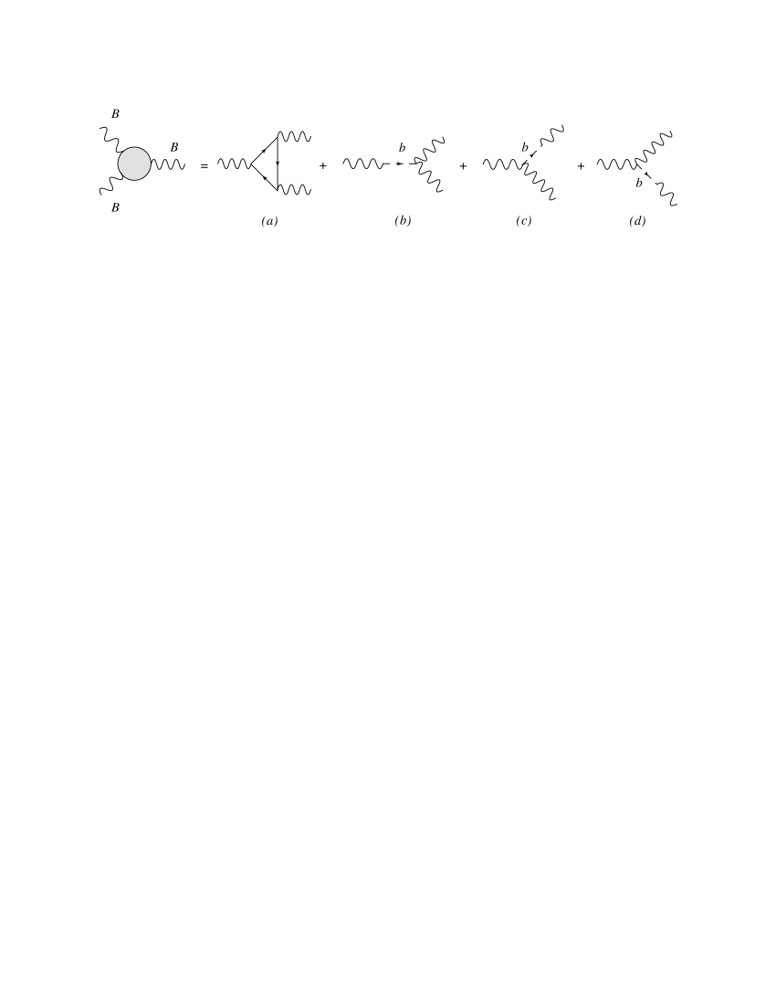
Figure 6: The GS vertex with the non-local contributions for the $BBB$ diagram symmetrized on each leg.

3.2 Non-local counterterms: axial QED

The use of non-local counterterms to cancel the anomaly is for sure a debated issue in quantum field theory since most of the results concerning the BRS analysis of these theories may not apply [14]. In the GS case we may ignore all the previous constructions and just require ab initio that the anomalous vertices are modified by the addition of a non-local counterterm that cancels the anomaly on the axial lines.

Consider, for instance, the case of the $BBB$ vertex of Fig.6, where the regularization of the anomalies has been obtained by adding the three GS counterterms in a symmetric way [20]. In the $BAA$ case only a single countertem is needed, but for the rest the discussion is quite similar to the $BBB$ case, with just a few differences. These concern the distribution of the partial anomalies on the A and B lines in the case in which also $BAA$ is treated symmetrically (equal partial anomalies). In this particular case we need to compensate the vertex with CS interactions, which are not, anyhow, observable if the A lines correspond to conserved gauge currents such as in QED. In this situation the Ward identities would force the CS counterterms to vanish. We will stick to the consistent definition of the anomaly in which only $B$ carries the total anomaly $a_{n}$ and $A$ is anomaly-free. The counterterm used in the GS mechanism both for $BAA$ and $BBB$ is nothing else but the opposite of the Dolgov-Zakharov (DZ) expression [21], which in the $BAA$ case takes the form

$$C^{\lambda\mu\nu}_{AVV}(k,k_{1},k_{2})=-\frac{a_{n}}{k^{2}}k^{\lambda}\epsilon[\mu,\nu,k_{1},k_{2}].$$ (15)

In the BBB case a similar expression is obtained by creating a Bose symmetric combination of DZ poles,

$$C^{\lambda\mu\nu}_{AAA}(k,k_{1},k_{2})=-\left(\frac{1}{3}\frac{a_{n}}{k^{2}}k^{\lambda}\epsilon[\mu,\nu,k_{1},k_{2}]+\frac{1}{3}\frac{a_{n}}{k_{1}^{2}}k_{1}^{\mu}\epsilon[\nu,\lambda,k_{2},k]+\frac{1}{3}\frac{a_{n}}{k_{2}^{2}}k_{2}^{\nu}\epsilon[\lambda,\mu,k,k_{1}]\right).$$ (16)

We have denoted by $k$ the incoming momenta of the axial-vector vertex and by $k_{1}$ and $k_{2}$ the outgoing momenta of the vector vertices. We keep this notation also in the AAA case, since $k$ will denote the momentum exchange in the s-channel when we glue together these amplitudes to obtain an amplitude of BIM type; this, we will analyze in the next sections. These expressions are consistent with the following equations of the anomaly for the $BAA$ triangle

$$k_{1\mu}C^{\lambda\mu\nu}_{AVV}(k,k_{1},k_{2})=0,$$

$$k_{2\nu}C^{\lambda\mu\nu}_{AVV}(k,k_{1},k_{2})=0,$$

$$k_{\lambda}C^{\lambda\mu\nu}_{AVV}(k,k_{1},k_{2})=-a_{n}\epsilon[\mu,\nu,k_{1},k_{2}],$$

and for the $BBB$ anomalous triangle

$$k_{1\mu}C^{\lambda\mu\nu}_{AAA}(k,k_{1},k_{2})=-\frac{a_{n}}{3}\epsilon[\lambda,\nu,k,k_{2}],$$

$$k_{2\nu}C^{\lambda\mu\nu}_{AAA}(k,k_{1},k_{2})=-\frac{a_{n}}{3}\epsilon[\lambda,\mu,k,k_{1}],$$

$$k_{\lambda}C^{\lambda\mu\nu}_{AAA}(k,k_{1},k_{2})=-\frac{a_{n}}{3}\epsilon[\mu,\nu,k_{1},k_{2}].$$

So we can define a gauge invariant triangle amplitude, in both the $BBB$ and $BAA$ cases, by

$$\Delta^{\lambda\mu\nu\,GS}_{AAA}(k,k_{1},k_{2}) = \Delta^{\lambda\mu\nu}_{AAA}(k,k_{1},k_{2})+C^{\lambda\mu\nu}_{AAA}(k,k_{1},k_{2})$$

$$\Delta^{\lambda\mu\nu\,GS}_{AVV}(k,k_{1},k_{2}) = \Delta^{\lambda\mu\nu}_{AVV}(k,k_{1},k_{2})+C^{\lambda\mu\nu}_{AVV}(k,k_{1},k_{2}).$$

Notice that the (fermionic) triangle diagrams, in the symmetric limit $k_{1}^{2}=k_{2}^{2}=k_{3}^{2}$, is exactly the opposite of the DZ counterterms, as we will discuss in the next section,

$$\Delta_{AVV}(k_{1}^{2}=k_{2}^{2}=k^{2})=-C_{AVV}\qquad\Delta_{AAA}(k_{1}^{2}=k_{2}^{2}=k^{2})=-C_{AAA},$$ (20)

so the cancellation is identical at that point (only at that point), and the two vertices $\Delta^{GS}$ vanish. It is rather obvious that the cancellations of these poles in BIM amplitudes, corrected by the GS counterterms, is identical only for on-shell external gauge lines. It is also quite straightforward to realize that the massless $B$-model with the GS vertex correction is equivalent to axial QED corrected by a non-local term [6] that is described by the Lagrangian

$$\mathcal{L}_{5\,QED}=\overline{\psi}\left(i\not{\partial}+e\not{B}\gamma_{5}\right)\psi-\frac{1}{4}F_{B}^{2}$$ (21)

plus the counterterm

$$\mathcal{S}_{ct}=\frac{1}{24\pi^{2}}\langle\partial B(x)\square^{-1}(x-y)F(y)\wedge F(y)\rangle.$$ (22)

This theory is equivalent to the (local) formulation given in Eq. 5 and in [14], where the transversality constraint ($\partial B=0$) is directly imposed on the Lagrangian via a multiplier.

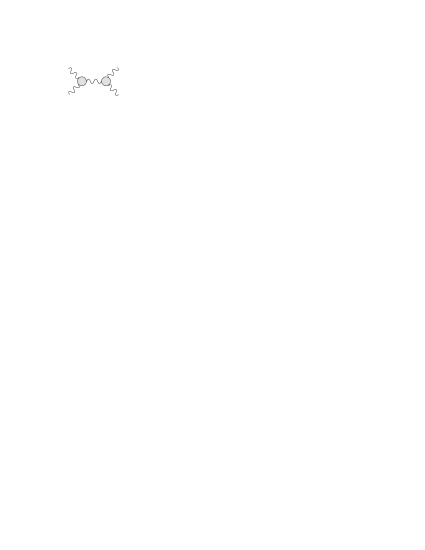
Figure 7: BIM-type amplitude with full GS vertices. For on-shell external lines the contributions from the extra poles disappear.

Figure 8: Embedding of the BIM amplitude with GS vertices in a fermion/antifermion scattering

Unitarity requires these DZ poles in the C counterterms to disappear from a physical amplitude. To show that this is not the case, in general, consider the diagrams depicted in Figs. 7 and 8. The structure of the GS vertex is, for $BBB$, given by (LABEL:reg1) with the three massless poles generated by the exchange of the pseudoscalar on the three legs, as shown in Fig. 6. For on-shell external lines, in this diagram the contributions from the extra poles cancel due to the transversality condition satisfied by the polarizators of the gauge bosons. However, once these amplitudes are embedded into more general amplitudes such as those shown in Fig. (8,9), the different virtualities of the momenta of the anomaly diagrams do not permit, in general, cancellation of the DZ extra poles introduced by the counterterm.

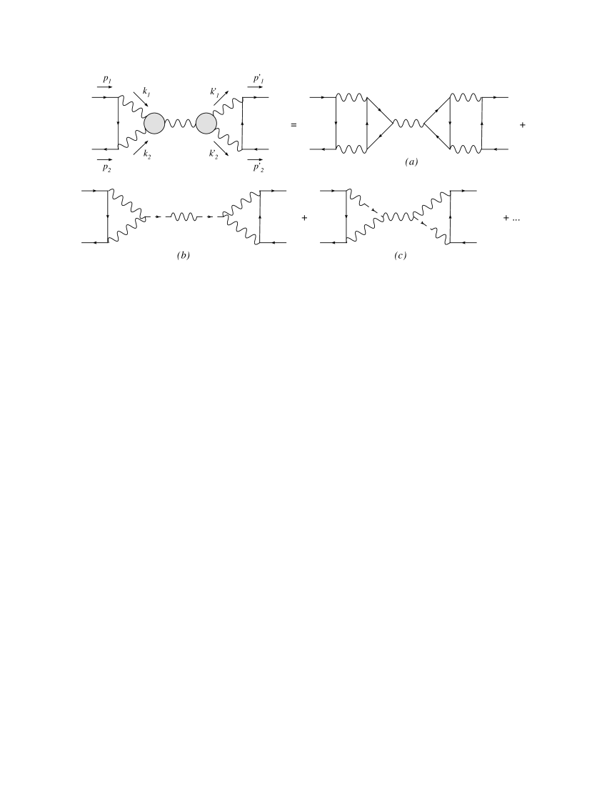
Figure 9: The structure of the fermionic scattering amplitudes with spurious massless poles (graphs b) and c)).

We can summarize the issues that we have raised in the following points.

1) The GS and the WZ mechanism have different formulations in terms of auxiliary fields.

2) Previous analyses of axial gauge theories, though distinct in their Lagrangian formulation, are all equivalent to axial QED plus a non-local counterterm. The regularization of the gauge interactions, in these theories, coincides with that obtained by using the GS counterterm on the gauge vertex. In particular, the massless poles introduced by the regularization are not understood in the context of perturbative unitarity.

A special comment is needed when we move to the analysis of Higgs- axion mixing. This has been shown to take place after electroweak symmetry breaking for a special class of potentials, which are not supersymmetric. The axion, which in the Stückelberg phase is essentially a Goldstone mode, develops a physical component and this component appears as a physical pole. It is then clear, from the analysis presented above, that the regularization procedure introduced by the GS counterterm involves a virtual massless state and not a physical pole. This is at variance with the WZ mechanism, in which the $bFF$ vertex is introduced from the beginning as a vertex and not just as a virtual state. In this second case, $b$ can be decomposed in terms of a Goldstone mode and a physical pseudoscalar, called in [7] the axi-Higgs, which takes the role of a gauged Peccei-Quinn axion [7]. This is entitled to appear as a physical state (and a physical pole, massless or massive) in the spectrum. The re-formulation of the GS counterterm in terms of a pseudoscalar comes also at a cost, due to the presence of a ghost (phantom) particle in the spectrum, which is absent in the WZ case. There are some advantages though, since the theory has, apparently, a nice ultraviolet behavior, given the gauge invariance condition on the vertex. The presence of these spurious poles requires further investigations to see how they are really embedded into higher order diagrams and we hope to return to this point in the near future in a related work. There is another observation on this issue that is worth to mention: the anomaly is also responsible for a UV/IR conspiracy which is puzzling on several grounds. For instance, the linear divergent terms $A_{1}$ and $A_{2}$ in the Rosenberg representation [22] of the anomaly diagram are closely related to the infrared anomaly poles in the amplitudes $A_{3}$ and $A_{6}$ in the chiral limit, due to the Ward identity[23].

In the next section we will move to the analysis of the unitarity bound in the WZ case. As we have shown, in this case it is possible to characterize it explicitly. We will work in a specific model, but the implications of our analysis are general and may be used to constrain significantly entire classes of models containing WZ interactions at the LHC. Before coming to the specific phenomenological applications we elaborate on the set of amplitudes that are instrumental in order to spot the bad high energy behavior of the chiral anomaly in s-channel processes: the BIM amplitudes.

4 BIM amplitudes, unitarity and the resonance pole

The uncontrolled growth of the cross section in the WZ case has to do with a certain class of amplitudes that have two anomalous (AVV or AAA ) vertices connected by an s-channel exchange as in Fig.3 a). We are interested in the expressions of these amplitudes in the chiral limit, when all the fermions are massless. Processes such as $AA\to AA$, mediated by an anomalous gauge boson $B$, with on-shell external A lines and massless fermions, can be expressed in a simplified form, which is, also in this case, the DZ form. We therefore set $k_{1}^{2}=k_{2}^{2}=0$ and $m_{f}=0$, which are the correct kinematical conditions to obtain DZ poles. We briefly elaborate on this point.

We start from the Rosenberg form of the $AVV$ amplitude, which is given by

$$T^{\lambda\mu\nu}=A_{1}\varepsilon[k_{1},\lambda,\mu,\nu]+A_{2}\varepsilon[k_{2},\lambda,\mu,\nu]+A_{3}k_{1}^{\mu}\varepsilon[k_{1},k_{2},\nu,\lambda]$$

$$\hskip 28.45274pt+A_{4}k_{2}^{\mu}\varepsilon[k_{1},k_{2},\nu,\lambda]+A_{5}k_{1}^{\nu}\varepsilon[k_{1},k_{2},\mu,\lambda]+A_{6}k_{2}^{\nu}\varepsilon[k_{1},k_{2},\mu,\lambda]\,,$$ (23)

and imposing the Ward identities we obtain

$$A_{1}=k_{2}^{2}A_{4}+k_{1}\cdot k_{2}A_{3}$$

$$A_{2}=k_{1}^{2}A_{5}+k_{1}\cdot k_{2}A_{6}$$

$$A_{3}(k_{1},k_{2})=-A_{6}(k_{1},k_{2})$$

$$A_{4}(k_{1},k_{2})=-A_{5}(k_{1},k_{2}),$$ (24)

where the invariant amplitudes $A_{3},\dots,A_{6}$ are free from singularities. In this specific kinematical limit we can use the following relations to simplify our amplitude

$$\varepsilon[k_{2},\lambda,\mu,\nu]=\frac{2}{s}\left(k_{2}^{\lambda}\varepsilon[k_{1},k_{2},\nu,\mu]+k_{2}^{\nu}\varepsilon[k_{1},k_{2},\mu,\lambda]+k_{2}^{\mu}\varepsilon[k_{1},k_{2},\nu,\lambda]\right)$$

$$\varepsilon[k_{1},\lambda,\mu,\nu]=-\frac{2}{s}\left(k_{1}^{\lambda}\varepsilon[k_{1},k_{2},\nu,\mu]+k_{1}^{\nu}\varepsilon[k_{1},k_{2},\mu,\lambda]+k_{1}^{\mu}\varepsilon[k_{1},k_{2},\nu,\lambda]\right)$$ (25)

where $k^{2}=(k_{1}+k_{2})^{2}=s$ is the center of mass energy. These combinations allow us to re-write the expression of the trilinear amplitude as

$$T^{\mu\nu\lambda}=A_{6}k^{\lambda}\varepsilon[k_{1},k_{2},\nu,\mu]+\left(A_{4}+A_{6}\right)\left(k_{2}^{\nu}\varepsilon[k_{1},k_{2},\mu,\lambda]-k_{1}^{\mu}\varepsilon[k_{1},k_{2},\nu,\lambda]\right)\,.$$ (26)

It is not difficult to see that the second piece drops off for physical external on-shell A lines, and we see that only one invariant amplitude contributes to the result

$$T^{\mu\nu\lambda}=A_{6}^{f}(s)(k_{1}+k_{2})^{\lambda}\varepsilon\left[k_{1},k_{2},\nu,\mu\right].$$ (27)

There are some observations to be made concerning this result. Notice that $A_{6}$ multiplies a longitudinal momentum exchange and, as discussed in the literature on the chiral anomaly in QCD [21, 24, 25], brings about a massless pole in $s$. We just recall that $A_{6}$ satisfies an unsubtracted dispersion relation in $s$ at a fixed invariant mass of the two photons, $(k_{1}^{2}=k_{2}^{2}=p^{2})$

$$A_{6}(s,p^{2})=\frac{1}{\pi^{2}}\int_{4m_{f}^{2}}^{\infty}dt\,\frac{{\it Im}A_{6}(t,p^{2})}{t-s}$$ (28)

and a sum rule

$$\int_{4m_{f}^{2}}^{\infty}ImA_{6}(t,p^{2})\,dt=\frac{1}{2\pi},$$ (29)

while for on-shell external photons one can use the DZ relation [21]

$$ImA_{6}(k^{2},0)=\frac{1}{\pi}\delta(k^{2}),$$ (30)

to show that the only pole of the amplitude is actually at $s=k^{2}=0$. It can be simplified using the identity

$$Li_{2}(1-a)+Li_{2}(1-a^{-1}) = -\frac{1}{2}\log^{2}(a),$$ (31)

with

$$a=\frac{\rho_{f}+1}{\rho_{f}-1}\qquad\rho_{f}=\sqrt{1-4\frac{m_{f}^{2}}{s}}\,,$$ (32)

to give [25]

$$A_{6}^{f}(s)=\frac{1}{2\pi^{2}s}\left(1-\frac{m_{f}^{2}}{s}\log^{2}\frac{\rho_{f}+1}{\rho_{f}-1}\right).$$ (33)

We can use this amplitude to discuss both the breaking of unitarity and the cancellation of the resonance pole in this simple model. The first point has already been addressed in the previous section, where the computation of the diagrams in Fig.2 has shown that only a BIM amplitude survives in the WZ case in the scattering process $AA\to AA$. If the sum of those two diagrams gives a gauge invariant result, with the exchange of the Z’ described by a Proca propagator, there is a third contribution that should be added to this amplitude. This comes from the exchange of the physical axion $\chi$. We recall, in fact, that in the presence of Higgs- axion mixing, when $b$ is the sum of a Goldstone mode and a physical axion $\chi$, each anomalous $Z^{\prime}$ is accompanied by the exchange of the $\chi$ [7]. This is generated in the presence of electroweak symmetry breaking, having expanded the Higgs scalar $\phi$ around a vacuum $v$

$$\phi=\frac{1}{\sqrt{2}}\left(v+\phi_{1}+i\phi_{2}\right),$$ (34)

with the axion $b$ expressed as linear combination of the rotated fields $\chi_{B}$ and $G_{B}$

$$b=\alpha_{1}\chi_{B}+\alpha_{2}G_{B}=\frac{q_{B}g_{B}v}{M_{B}}\chi_{B}+\frac{M_{1}}{M_{B}}G_{B}.$$ (35)

We also recall that the gauge fields $B_{\mu}$ get their masses $M_{B}$ through the combined Higgs-Stückelberg mechanism,

$$M_{B}=\sqrt{M_{1}^{2}+(q_{B}g_{B}v)^{2}}.$$ (36)

In the phenomenological analysis presented in the next sections the contribution due to $\chi$ has been included. Therefore, in the WZ case, the total contributions coming from the several BIM amplitudes related to the additional anomalous neutral currents should be accompanied not only by the set of Goldstone bosons, to restore gauge invariance, but also by the exchange of the axi-Higgs.

The cancellation of the resonance pole for $s=M_{B}$ is an important characteristic of BIM amplitudes, which does not occur in any other (anomaly-free) amplitude. This cancellation is the result of some amusingly trivial algebra which we reproduce just for the sake of clarity. Given a BIM amplitude and Proca exchange, we have

$$A_{BIM} = \frac{a_{n}}{k^{2}}k^{\lambda}\varepsilon[\mu,\nu,k_{1},k_{2}]\,\frac{-i}{k^{2}-M_{1}^{2}}\left(g^{\lambda\lambda^{\prime}}-\frac{k^{\lambda}k^{\lambda^{\prime}}}{M_{1}^{2}}\right)\frac{a_{n}}{k^{2}}(-k^{\lambda^{\prime}})\varepsilon[\mu^{\prime},\nu^{\prime},k_{1}^{\prime},k_{2}^{\prime}]$$ (37)

$$= \frac{a_{n}}{k^{2}}\varepsilon[\mu,\nu,k_{1},k_{2}]\,\frac{-i}{k^{2}-M_{1}^{2}}\frac{k^{\lambda^{\prime}}(M_{1}^{2}-k^{2})}{M_{1}^{2}}\,\frac{a_{n}}{k^{2}}(-k^{\lambda^{\prime}})\varepsilon[\mu^{\prime},\nu^{\prime},k_{1}^{\prime},k_{2}^{\prime}]$$

$$= \frac{a_{n}}{k^{2}}\varepsilon[\mu,\nu,k_{1},k_{2}]\,\left(\frac{-ik^{2}}{M_{1}^{2}}\right)\,\frac{a_{n}}{k^{2}}\varepsilon[\mu^{\prime},\nu^{\prime},k_{1}^{\prime},k_{2}^{\prime}]$$

$$= -\frac{a_{n}}{M_{1}}\varepsilon[\mu,\nu,k_{1},k_{2}]\,\,\frac{i}{k^{2}}\,\,\frac{a_{n}}{M_{1}}\varepsilon[\mu^{\prime},\nu^{\prime},k_{1}^{\prime},k_{2}^{\prime}].$$

This result implies that the amplitude is described - in the chiral limit and for massless external states - by a diagram with the exchange of a pseudoscalar (see Fig.2 b)) and that the resonance pole has disappeared. It is clear, from (37), that these amplitudes break unitarity and give a contribution to the cross section that grows quadratically in energy ($\sim s$). Therefore, searching for BIM amplitudes at the LHC can be a way to uncover the anomalous behavior of extra neutral (or charged) gauge interactions. There is one thing that might tame this growth, and this is the exchange of the physical axion. We will show, working in a complete brane model, that the exchange of the $\chi$ does lower the cross section, but insignificantly, independently from the mass of the axion.

5 A realistic model with WZ counterterms

Having clarified the relation between the WZ and GS mechanisms using our simple toy-model, we move towards the analysis of the issue of unitarity violation in the WZ Lagrangian at high energy. Details on the structure of the effective action of the complete model that we are going to analyze can be found in [9]. We just mention that this is characterized by a gauge structure of the form $SU(3)\times SU(2)\times U(1)\times U(1)_{B}$, where the $U(1)_{B}$ is anomalous. We work in the context of a two-Higgs doublet model with $H_{u}$ and $H_{d}$ [7]. In our analysis our setup is that of a complete model, in the sense that all the charge assignments are those of a realistic brane model with three extra anomalous $U(1)$, but we will, for simplicity, assume that only the lowest mass eigenvalue taking part is significant, since the remaining two additional gauge bosons are heavy and, essentially, decoupled.

We recall that the single anomalous gauge boson, $B$, that we consider in this analysis is characterized by a generator $Y_{B}$, which is anomalous ($TrY_{B}^{3}\neq 0$) but at the same time has mixed anomalies with the remaining generators of SM and in particular with the hypercharge, $Y$. In the presence of a single anomalous $U(1)$, here denoted as $U(1)_{B}$, both the $Z$ and the (extra) $Z^{\prime}$ gauge boson have an anomalous component, proportional to $B$. We also recall that the effective action of the anomalous theory is rendered gauge invariant using both CS and Green-Schwarz counterterms, while a given gauge invariant sector involves the exchange both of the anomalous gauge boson and of the axion in the $s$-,$t$- and $u$-channels.

In a previous work [10] it has been shown how the trilinear vertices of the effective WZ Lagrangian can be determined consistently for a generic number of extra anomalous $U(1)$. Here, the goal is to identify and quantify the contributions that cause a violation of unitarity in this Lagrangian. For phenomenological reasons it is then convenient to select those BIM amplitudes that have a better chance, at the experimental level, to be measured at the LHC and for this reason we will focus on the process $g\,g\to\gamma\gamma$. The gluon density grows at high energy especially at smaller (Bjorken variable) $x$-values. We choose to work with prompt final state photons for obvious reasons, the signal being particularly clean. To begin with, we will be needing the expressions of the $Z\gamma\gamma$ and the $Zgg$ vertices. In the presence of three anomalous $U(1)$, here denoted as $U(1)_{B}$, both the $Z$ and the (extra) $Z^{\prime}$ gauge boson have an anomalous component, which is proportional to the $B_{i\mu}$, the anomalous gauge bosons of the interaction eigenstate basis (i=1,2,3). The photon vertex is given by [10]

$$\langle Z_{l}\gamma\gamma\rangle|_{m_{f}\neq 0}=-\frac{1}{2}Z^{\lambda}_{l}A_{\gamma}^{\mu}A_{\gamma}^{\nu}\sum_{f}\left[g_{Y}^{3}\theta_{f}^{YYY}\bar{R}^{YYY}_{Z_{l}\gamma\gamma}+g_{2}^{3}\theta_{f}^{WWW}\bar{R}^{WWW}_{Z_{l}\gamma\gamma}+g_{Y}g_{2}^{2}\theta_{f}^{YWW}R^{YWW}_{Z_{l}\gamma\gamma}\right.$$

$$\hskip 56.9055pt\left.+g_{Y}^{2}g_{2}\theta_{f}^{YYW}R^{YYW}_{Z_{l}\gamma\gamma}+\sum_{i}g_{B_{i}}g_{Y}g_{2}\theta_{f}^{B_{i}YW}R^{B_{i}YW}_{Z_{l}\gamma\gamma}\right.$$

$$\hskip 56.9055pt\left.+\sum_{i}g_{B_{i}}g_{Y}^{2}\theta_{f}^{B_{i}YY}R^{B_{i}YY}_{Z_{l}\gamma\gamma}+g_{B_{i}}g_{2}^{2}\theta_{f}^{B_{i}WW}R^{B_{i}WW}_{Z_{l}\gamma\gamma}\right]\Delta_{AVV}^{\lambda\mu\nu}(m_{f}\neq 0).$$

with $l=1,2,3$ enumerating the extra anomalous neutral currents. The explicit expressions of the rotation matrix $O^{A}$ can be found in [9, 10]. We have defined

$$\bar{R}^{YYY}_{Z_{l}\gamma\gamma}=(O^{A})_{YZ_{l}}(O^{A})_{Y\gamma}^{2},\hskip 28.45274pt\bar{R}^{WWW}_{Z_{l}\gamma\gamma}=(O^{A})_{W_{3}Z_{l}}(O^{A})_{W_{3}\gamma}^{2},$$ (39)

and the triangle $\Delta_{AVV}(m_{f}\neq 0)$ is given by [10]

$$\Delta_{AVV}^{\lambda\mu\nu}(m_{f}\neq 0,k_{1},k_{2})=\frac{1}{\pi^{2}}\int_{0}^{1}dx\int_{0}^{1-x}dy\frac{1}{\Delta(m_{f})}$$

$$\hskip 56.9055pt\left\{\varepsilon[k_{1},\lambda,\mu,\nu]\left[y(y-1)k_{2}^{2}-xyk_{1}\cdot k_{2}\right]\right.$$

$$\hskip 56.9055pt\left.+\varepsilon[k_{2},\lambda,\mu,\nu]\left[x(1-x)k_{1}^{2}+xyk_{1}\cdot k_{2}\right]\right.$$

$$\hskip 56.9055pt\left.+\varepsilon[k_{1},k_{2},\lambda,\nu]\left[x(x-1)k_{1}^{\mu}-xyk_{2}^{\mu}\right]\right.$$

$$\hskip 56.9055pt\left.+\varepsilon[k_{1},k_{2},\lambda,\mu]\left[xyk_{1}^{\nu}+(1-y)yk_{2}^{\nu}\right]\right\}\,,$$

$$\Delta(m_{f})=m_{f}^{2}+x(x-1)k_{1}^{2}+y(y-1)k_{2}^{2}-2xyk_{1}\cdot k_{2}\,.$$ (40)

We have defined the following chiral asymmetries

$$\theta^{B_{l}YY}_{f}=Q_{B_{j},f}^{L}(Q_{Y,f}^{L})^{2}-Q_{B_{l},f}^{R}(Q_{Y,f}^{R})^{2},$$

$$\theta^{B_{l}WW}_{f}=Q_{B_{l},f}^{L}(T^{3}_{L,f})^{2},$$

$$\theta_{f}^{WWW}=(T^{3}_{L,f})^{3},$$

$$\theta_{f}^{YYW}=\left[(Q^{L}_{Y,f})^{2}T^{3}_{L,f}\right],$$

$$\theta_{f}^{B_{l}YW}=\left[Q^{B_{l},f}Q^{L}_{Y,f}T^{3}_{L,f}\right],$$ (41)

with $Q_{B}^{L/R}$ and $Q_{Y}^{L/R}$ denoting the charges of the chiral fermions and $T^{3}_{L}$ is the generator of the third component of the weak isospin, while the $R$ factors are products of $O^{A}$ matrix elements. The matrix $O^{A}$ relates the interaction eigenstate basis of the generators $(Y_{B},Y,T_{3})$ to those of the mass eigenstate basis $(T_{Z},T_{Z^{\prime}},Q)$, of the physical gauge bosons of the neutral sector, $Z,Z^{\prime}$ and $A_{\gamma}$. They are given by

$$R^{YYY}_{Z_{l}\gamma\gamma}=3\left[(O^{A})_{YZ_{l}}(O^{A})_{Y\gamma}^{2}\right]$$

$$R^{YWW}_{Z_{l}\gamma\gamma}=\left[2(O^{A})_{W_{3}\gamma}(O^{A})_{YZ_{l}}(O^{A})_{Y\gamma}+(O^{A})_{W_{3}\gamma}^{2}(O^{A})_{YZ_{l}}\right]$$

$$R^{WWW}_{Z_{l}\gamma\gamma}=\left[3(O^{A})_{B_{i}Z_{l}}(O^{A})^{2}_{W_{3}\gamma}\right]$$

$$R^{YYW}_{Z_{l}\gamma\gamma}=\left[2(O^{A})_{YZ_{l}}(O^{A})_{Y\gamma}(O^{A})_{W_{3}\gamma}+(O^{A})_{W_{3}Z_{l}}(O^{A})_{Y\gamma}^{2}\right]$$

$$R^{B_{i}YY}_{Z_{l}\gamma\gamma}=(O^{A})_{Y\gamma}^{2}(O^{A})_{B_{i}Z_{l}}$$

$$R^{B_{i}WW}_{Z_{l}\gamma\gamma}=\left[(O^{A})_{W_{3}\gamma}^{2}(O^{A})_{B_{i}Z_{l}}\right]$$

$$R^{B_{i}YW}_{Z_{l}\gamma\gamma}=\left[2(O^{A})_{B_{i}Z_{l}}(O^{A})_{W_{3}\gamma}(O^{A})_{Y\gamma}\right]\,.$$

These expressions will be used extensively in the next section and computed numerically in a complete brane model.

5.0.1 MLSOM with one Higgs doublet and an extra singlet

Another possible framework for the Higgs sector is to consider a Lagrangian containing one $SU(2)_{W}$ Higgs doublet $H_{u}$ and an extra singlet $\phi$.

In this context all the features concerning the mass matrix for the gauge bosons remain the same, in fact the covariant derivatives act on the fields as follows

$${\cal D}_{\mu}H_{u}=\left(\partial_{\mu}+ig_{2}\frac{\tau^{i}}{2}W^{i}_{\mu}+ig_{Y}q_{u}^{Y}A^{Y}_{\mu}+ig_{B}\frac{q_{u}^{B}}{2}B_{\mu}\right)H_{u},$$

$${\cal D}_{\mu}\phi=\left(\partial_{\mu}+ig_{Y}q_{\phi}^{Y}A^{Y}_{\mu}+ig_{B}\frac{q_{\phi}^{B}}{2}B_{\mu}\right)\phi\,,$$ (43)

where $q_{u}^{B}$ and $q_{\phi}^{B}$ are respectively the charges of the higgs fields under the extra anomalous $U(1)$ symmetry.

After the spontaneous symmetry breaking, expanding around the vacuum of the two Higgs bosons, we have

$$H^{0}_{u}=v_{u}+\frac{\mbox{Re}H_{u}^{0}+i\mbox{Im}{H_{u}^{0}}}{\sqrt{2}}, \phi=v_{\phi}+\frac{\mbox{Re}{\phi}+i\mbox{Im}{\phi}}{\sqrt{2}}\,.$$ (44)

By this procedure we obtain a $3\times 3$ mass matrix in the mixing of the neutral gauge bosons, which is similar to that obtained in [9].

In the Higgs sector the structure of the Peccei-Quinn potential is similar to that obtained in the presence of two Higgs doublets. In fact, the symmetric potential is given by

$$V_{PQ}=\mu_{u}^{2}H_{u}^{\dagger}H_{u}+\lambda_{uu}(H_{u}^{\dagger}H_{u})^{2}-2\lambda_{u\phi}(H_{u}^{\dagger}H_{u})\phi^{*}\phi+\mu_{\phi}^{2}\phi^{*}\phi+\lambda_{\phi\phi}(\phi^{*}\phi)^{2}\,,$$ (45)

where the coefficients $\mu_{u}$ and $\mu_{\phi}$ have mass dimension 1 and $\lambda_{uu},\lambda_{u\phi},\lambda_{\phi\phi}$ are dimensionless, while the PQ breaking terms can be written as

$$V_{P\kern-3.01389pt\hbox{/}Q\kern-3.01389pt\hbox{/}}=\bar{\mu}(H^{\dagger}_{u}H_{u})\phi~{}e^{iq^{B}_{\phi}\frac{b}{M_{1}}}+\bar{\lambda}(\phi^{*}\phi)\phi~{}e^{iq^{B}_{\phi}\frac{b}{M_{1}}}+\textrm{c.c.}\,,$$ (46)

where $\bar{\mu}$ and $\bar{\lambda}$ have mass dimension 1. The $CP$-odd sector is still characterized by a $3\times 3$ matrix similar to $O^{\chi}$, which we call for simplicity $O^{\prime\chi}$; this allows for the rotation from the interaction eigenstates basis to the physical basis, as follows

$$\left(\begin{array}[]{c}\mbox{Im}H^{0}_{u}\\ \mbox{Im}\phi\\ b\end{array}\right)=O^{\prime\chi}\left(\begin{array}[]{c}\chi\\ G^{0}_{1}\\ G^{0}_{2}\end{array}\right)\,.$$

Therefore, in this picture the spectrum in this sector is unchanged, we have a physical axion and its mass exhibits a combination of two effects, the Higgs vevs and the presence of a PQ breaking potential. The parameters can be tuned to be small enough to have a light physical axion. In general, bounds coming from experimental, astrophysical and cosmological sources give an upper limit for the axion mass, which is around $10$ meV  [26],[27].

5.1 Prompt photons, the Landau-Yang theorem and the anomaly

Since the analysis of the unitarity bound will involve the study of amplitudes with direct photons in the final state mediated by a $Z$ or a $Z^{\prime}$ in the s-channel, we briefly recall some facts concerning the structure of these amplitude and in particular the Landau-Yang theorem. The condition of transversality of the $Z^{\prime}$ boson ($e_{Z^{\prime}}\cdot k=0$) is essential for the vanishing of this amplitude. A direct proof of the vanishing of the on-shell vertex can be found in [11, 9].

The theorem states that a spin 1 particle cannot decay into two on-shell spin 1 photons because of Bose symmetry and angular momentum conservation. Angular momentum conservation tells us that the two photons must be in a spin 1 state (which forces their angular momentum wave function to be antisymmetric), while their spatial part is symmetric. The total wave function is therefore antisymmetric and violates the requirement of Bose statistics. For these reasons the amplitude has to vanish. For a virtual exchange mediated by a $Z^{\prime}$ the contribution is vanishing -after summing over the fermions in each generation of the SM-, the theory being anomaly-free, in the chiral limit. The amplitude is non-vanishing only in the presence of chiral symmetry breaking terms (fermion masses), which can be induced both by the QCD vacuum and by the Yukawa couplings of SM in the presence of electroweak symmetry breaking. For this reason it is strongly suppressed also in the SM.

However, the situation in the case of an anomalous vertex is more subtle. The BIM amplitude is non-vanishing, but at the same time, as we have explained, is non-resonant, which means that the particle pole due to the $Z^{\prime}$ has disappeared. For the rest it will break unitarity at a certain stage.

In fact, a cursory look at the AVV vertex shows that if the external photons are on-shell and transverse, the amplitude mediated by this diagram is proportional to the momentum of the virtual $Z$, $k^{\mu}$. This longitudinal momentum exchange does not set the amplitude to $0$ unless the production mechanism is also anomalous. We will show first that in the SM these processes are naturally suppressed, though not identically $0$, since they are proportional to the fermion masses, due to anomaly cancellation. We start our analysis by going back to the AVV diagram, which summarizes the kinematical behavior of the $Z\gamma\gamma$ amplitude.

Let $k_{1}$ and $k_{2}$ denote the momenta of the two final state photons. We contract the AVV diagram with the polarization vectors of the photons, $\varepsilon_{1\mu}$ and $\varepsilon_{2\nu}$ of the $Z$ boson, $e_{\lambda}$, obtaining

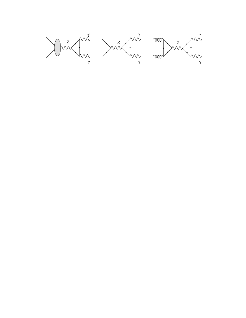
Figure 10: Vanishing and non-vanishing amplitudes mediated by an axial-vector spin 1.

$$e_{\lambda}\varepsilon_{1\mu}\varepsilon_{2\nu}\Delta_{AVV}^{\lambda\mu\nu}(k_{1},k_{2},m_{f}\neq 0)=-\frac{1}{\pi^{2}}\int_{0}^{1}dx\int_{0}^{1-x}dy\frac{xy}{m_{f}^{2}-2xyk_{1}\cdot k_{2}}$$

$$\hskip 56.9055pte_{\lambda}\varepsilon_{1\mu}\varepsilon_{2\nu}\left\{\varepsilon_{\lambda\nu\mu\alpha}\left(k_{2}^{\alpha}-k_{1}^{\alpha}\right)+k_{1}^{\alpha}k_{2}^{\beta}\left(\varepsilon_{\alpha\lambda\beta\nu}k_{2}^{\mu}-\varepsilon_{\alpha\lambda\beta\mu}k_{1}^{\nu}\right)\right\}\,,$$ (47)

where we have used the conditions

$$k_{1}^{2}=k_{2}^{2}=0$$

$$\varepsilon_{1\mu}k_{1}^{\mu}=\varepsilon_{2\nu}k_{2}^{\nu}=0.$$ (48)

It is important to observe that if we apply Schouten’s identity we can reduce this expression to the form

$$e_{\lambda}\varepsilon_{1\mu}\varepsilon_{2\nu}\Delta_{AVV}^{\lambda\mu\nu}(k_{1},k_{2},m_{f}\neq 0)=e_{\lambda}\left(k_{1}^{\lambda}+k_{2}^{\lambda}\right)\mathcal{F}_{f}(k^{2},m_{f})$$ (49)

with

$$\mathcal{F}_{f}(k^{2},m_{f}) = \mathcal{J}_{f}(k^{2})\varepsilon[k_{1},k_{2},\varepsilon_{1},\varepsilon_{2}]$$

$$\mathcal{J}_{f}(k^{2}) \equiv -\frac{1}{\pi^{2}}\int_{0}^{1}dx\int_{0}^{1-x}dy\frac{xy}{m_{f}^{2}-2xyk_{1}\cdot k_{2}},$$ (50)

which vanishes only if we impose the transversality condition on the polarization vector of the $Z$ boson, $e_{\lambda}k^{\lambda}=0$. Alternatively, this amplitude vanishes if the anomalous $Z$-photon-photon vertex is contracted with another gauge invariant vertex, as discussed above. The amplitude has an anomalous behavior. In fact, contracting with the $k_{\lambda}$ four-vector we obtain

$$k_{\lambda}\varepsilon_{1\mu}\varepsilon_{2\nu}\Delta_{AVV}^{\lambda\mu\nu}(k_{1},k_{2},m_{f}\neq 0)=\left(-\frac{1}{\pi^{2}}\int_{0}^{1}dx\int_{0}^{1-x}dy\frac{k_{\lambda}k^{\lambda}xy}{m_{f}^{2}-2xyk_{1}\cdot k_{2}}\right)\varepsilon[k_{1},k_{2},\varepsilon_{1},\varepsilon_{2}]$$

$$\hskip 28.45274pt=\left(\frac{1}{\pi^{2}}\int_{0}^{1}dx\int_{0}^{1-x}dy\frac{-2k_{1}\cdot k_{2}xy}{m_{f}^{2}-2xyk_{1}\cdot k_{2}}\right)\varepsilon[k_{1},k_{2},\varepsilon_{1},\varepsilon_{2}]$$

$$\hskip 28.45274pt=\left(\frac{1}{\pi^{2}}+\frac{m_{f}^{2}}{\pi^{2}}\int_{0}^{1}dx\int_{0}^{1-x}dy\frac{1}{m_{f}^{2}-2xyk_{1}\cdot k_{2}}\right)\varepsilon[k_{1},k_{2},\varepsilon_{1},\varepsilon_{2}]$$ (51)

where the mass-independent and mass-dependent contributions have been separated. Summing over an anomaly-free generation, the first of these two contributions cancel.

For this reason, it is also convenient to isolate the following quantity

$${\mathcal{G}}_{f}(k^{2},m_{f})=\frac{m_{f}^{2}}{\pi^{2}}\int_{0}^{1}dx\int_{0}^{1-x}dy\frac{1}{m_{f}^{2}-2xyk_{1}\cdot k_{2}}\varepsilon[k_{1},k_{2},\varepsilon_{1},\varepsilon_{2}]$$ (52)

which is the only contribution to the triangle amplitude in the SM for a given fermion flavor $f$.

We illustrate in Fig.10 the contributions to the $q\bar{q}$ annihiliation channel at all orders (first graph), at leading order (second graph), and the BIM amplitude (third graph), all attached to an $AVV$ final state. In an anomaly-free theory all these processes are only sensitive to the difference in masses among the flavors, since degeneracy in the fermion mass sets these contributions to zero. Only the second graph vanishes identically due to the Ward identity on the $q\bar{q}$ channel also away from the chiral limit. For instance in the third diagram chiral symmetry breaking is sufficient to induce violations of the Ward identity on the initial state vertex, due to the different quark masses within a given fermion generation.

To illustrate, in more detail, how chiral symmetry breaking can induce the exchange of a scalar component in the process with two prompt photons, we start from the SM case, where the $Z^{*}\gamma\gamma$ vertex, multiplied by external physical polarizations for the two photons becomes

$$V^{\lambda}_{Z^{*}\gamma\gamma}=k^{\lambda}\frac{g_{2}}{2\cos{\theta}_{W}}e^{2}\sum_{f}(Q_{f})^{2}g_{A,f}^{Z}\mathcal{F}_{f}(k^{2},m_{f})$$ (53)

and consider the quark antiquark annihilation channel $q\bar{q}\rightarrow Z^{*}\rightarrow\gamma\gamma$. We work in the parton model with massless light quarks. We can rewrite the amplitude as

$$\mathcal{M} = V^{\lambda}_{ffZ^{*}}\Pi_{\lambda,\lambda^{\prime},\xi}V^{\lambda^{\prime}}_{Z^{*}\gamma\gamma},$$ (54)

where we have introduced the $Zq\bar{q}$ vertex

$$V_{ffZ}=\bar{v}(p_{1})\Gamma^{\lambda^{\prime}}u(p_{2})\hskip 28.45274pt\Gamma^{\lambda}=ig_{Z}\gamma^{\lambda}(g_{V}-g_{A}\gamma^{5}),$$ (55)

and the expression of the propagator of the $Z$ in the $R_{\xi}$ gauge

$$\Pi_{\lambda,\lambda^{\prime},\xi}=\frac{-i}{k^{2}-M_{Z}^{2}}\left[g^{\lambda\lambda^{\prime}}-\frac{k^{\lambda}k^{\lambda^{\prime}}}{k^{2}-\xi M_{Z}^{2}}(1-\xi)\right].$$ (56)

To move to the unitary gauge, we split the propagator of the $Z$ as

$$\Pi_{\lambda,\lambda^{\prime},\xi}=\frac{-i}{k^{2}-M_{Z}^{2}}\left[g^{\lambda\lambda^{\prime}}-\frac{k^{\lambda}k^{\lambda^{\prime}}}{M_{Z}^{2}}\right]+\frac{-i}{k^{2}-\xi M_{Z}^{2}}\left(\frac{k^{\lambda}k^{\lambda^{\prime}}}{M_{Z}^{2}}\right)$$ (57)

and go to the unitary gauge by choosing $\xi\rightarrow\infty$. The amplitude will then be written as

$${\cal M} = \bar{v}(p_{1})\Gamma^{\lambda}u(p_{2})\frac{-i}{k^{2}-M_{Z}^{2}}\left[g^{\lambda\lambda^{\prime}}-\frac{k^{\lambda}k^{\lambda^{\prime}}}{M_{Z}^{2}}\right]k^{\lambda^{\prime}}\left(\frac{g_{2}}{2\cos{\theta}_{W}}e^{2}\sum_{f}(Q_{f})^{2}g_{A,f}^{Z}\mathcal{F}_{f}(k^{2},m_{f})\right)$$

$$= \frac{i}{M_{Z}^{2}}\bar{v}(p_{1})\Gamma^{\lambda}u(p_{2})k^{\lambda}\left(\frac{g_{2}}{2\cos{\theta}_{W}}e^{2}\sum_{f}(Q_{f})^{2}g_{A,f}^{Z}\mathcal{F}_{f}(k^{2},m_{f})\right).$$

Clearly, at the Born level, using the Ward identity on the left $V_{ffZ^{*}}$ vertex, we find that the amplitude is zero. This result remains unchanged if we include higher order corrections (strong/electroweak), since the structure of this vertex is just modified by a Pauli (weak-electric) form factor and the additional contribution vanishes after contraction with the momentum $k^{\lambda}$.

Figure 11: Anomalous contributions in $gg\to\gamma\gamma$

This amplitude is however non-vanishing if we replace the $V_{ffZ^{*}}$ vertex with a $V_{ggZ^{*}}$ vertex, where now we assume that the new vertex is computed for non-zero fermion masses (i.e. away from the chiral limit). In this case we use the Ward identity

$$k_{\rho}\,V_{ggZ^{*}}^{\rho\nu\mu} = (p_{1}+p_{2})_{\rho}\,G^{\,\rho\nu\mu}$$ (59)

$$= -\frac{e^{2}g_{2}}{2\cos\theta_{W}}\sum_{q}g^{Z}_{A,q}Q^{2}_{q}\,\epsilon^{\,\nu\mu\alpha\beta}p_{1\alpha}p_{2\beta}\,\left[\frac{1}{\pi^{2}}+\frac{m^{2}_{q}}{\pi^{2}}\int^{1}_{0}dx_{1}\int^{1-x_{1}}_{0}dx_{2}\,\frac{1}{\Delta_{q}}\right]$$

with

$$\Delta_{q}=-xyk^{2}+m_{q}^{2},$$ (60)

where the constant term $(1/\pi^{2})$ vanishes in an anomaly-free theory. It is convenient to define the function

$$\mathcal{G}_{q}(k^{2},m_{q})=\epsilon\left[\varepsilon_{1g},\varepsilon_{2g},p_{1},p_{2}\right]m^{2}_{q}\mathcal{I}_{q}(m_{q})$$ (61)

with

$$\mathcal{I}_{q}(m_{q})=\frac{1}{\pi^{2}}\int^{1}_{0}dx_{1}\int^{1-x_{1}}_{0}dx_{2}\,\frac{1}{\Delta_{q}},$$ (62)

where $\varepsilon$ is the polarization of the gluon, which allows one to express the squared amplitude as

$$\langle|\mathcal{M}_{gg\to\gamma\gamma}|^{2}\rangle = \left(\frac{e^{2}g_{2}}{2\cos\theta_{W}}\right)^{4}\frac{s^{6}}{4M_{Z}^{4}}\left(\sum_{q}g^{q}_{A}Q^{2}_{q}\mathcal{G}_{q}(m_{q})\right)^{2}\left(\sum_{f}g^{f}_{A}Q^{2}_{f}\mathcal{G}_{f}(m_{f})\right)^{2},$$

with $s\equiv k^{2}$. Notice that in the large energy limit $\mathcal{I}_{q}\sim\mathcal{J}_{f}\sim 1/{s^{2}}$ [25]. This shows that double prompt photon production, in the SM, is non-resonant and is proportional to the quark masses, neglecting the contributions coming from the masses of the leptons.

6 Gauge parameter dependence in the physical basis

When this analysis is extended to a complete anomalous model such as the MLSOM [7, 9, 10] even the direct proof of the cancellation of the gauge dependence in the $Z^{\prime}$ exchange is quite complex and not obvious, although it is expected at a formal level. We recall that we are working with a broken phase and the axion has been decomposed into its physical component ($\chi$, which is the axi-Higgs) and the Goldstone modes of the extra $Z^{\prime}$, $G_{Z^{\prime}}$. In [10] it has been shown that the counterterms of the theory can be fixed in the Stückelberg phase and then re-expressed, in the Higgs-Stückelberg phase, in the physical base. Although the procedure is formally correct, the explicit check of cancellation of these gauge dependences is far from trivial and is based on some identities that we have been able to derive after some efforts, which confirm the correctness of the approach followed in [9, 10] for the determination of the effective Lagrangian of the model after electroweak symmetry breaking.

The matrix $O^{\chi}$, needed to rotate into the mass eigenstates of the $CP$-odd sector, relating the axion $\chi$ and the two neutral Goldstones of this sector to the Stückelberg field $b$ and the $CP$-odd phases of the two Higgs doublets satisfies the following relation

$$\left(\begin{array}[]{c}ImH^{0}_{u}\\ ImH^{0}_{d}\\ b\end{array}\right)=O^{\chi}\left(\begin{array}[]{c}\chi\\ G^{0}_{1}\\ G^{0}_{2}\end{array}\right)\,,$$

where the Goldstones in the physical basis are obtained by the following combination

$$G^{Z} = G^{0}_{1}\left[f_{u}\frac{v_{u}}{M_{Z}}O^{\chi}_{12}+f_{d}\frac{v_{d}}{M_{Z}}O^{\chi}_{22}+g_{B}\frac{M_{1}}{M_{Z}}O^{A}_{ZB}O^{\chi}_{32}\right]$$

$$+ G^{0}_{2}\left[f_{u}\frac{v_{u}}{M_{Z}}O^{\chi}_{13}+f_{d}\frac{v_{d}}{M_{Z}}O^{\chi}_{23}+g_{B}\frac{M_{1}}{M_{Z}}O^{A}_{ZB}O^{\chi}_{33}\right]$$

$$= c_{1}G^{0}_{1}+c_{2}G^{0}_{2}$$

$$G^{Z^{\prime}} = G^{0}_{1}\left[f_{u,B}\frac{v_{u}}{M_{Z}^{\prime}}O^{\chi}_{12}+f_{d,B}\frac{v_{d}}{M_{Z}^{\prime}}O^{\chi}_{22}+g_{B}\frac{M_{1}}{M_{Z}^{\prime}}O^{A}_{Z^{\prime}B}O^{\chi}_{32}\right]$$ (64)

$$+ G^{0}_{2}\left[f_{u,B}\frac{v_{u}}{M_{Z}^{\prime}}O^{\chi}_{13}+f_{d,B}\frac{v_{d}}{M_{Z}^{\prime}}O^{\chi}_{23}+g_{B}\frac{M_{1}}{M_{Z}^{\prime}}O^{A}_{Z^{\prime}B}O^{\chi}_{33}\right]$$

$$= c^{\prime}_{1}G^{0}_{1}+c^{\prime}_{2}G^{0}_{2}\,.$$

Here we have defined the following coefficients

$$f_{u}=g_{2}O^{A}_{ZW_{3}}-g_{Y}O^{A}_{ZY}-q^{B}_{u}g_{B}O^{A}_{ZB} f_{d}=g_{2}O^{A}_{ZW_{3}}-g_{Y}O^{A}_{ZY}-q^{B}_{d}g_{B}O^{A}_{ZB}$$

$$f_{u,B}=g_{2}O^{A}_{Z^{\prime}W_{3}}-g_{Y}O^{A}_{Z^{\prime}Y}-q^{B}_{u}g_{B}O^{A}_{Z^{\prime}B} f_{d,B}=g_{2}O^{A}_{Z^{\prime}W_{3}}-g_{Y}O^{A}_{Z^{\prime}Y}-q^{B}_{d}g_{B}O^{A}_{Z^{\prime}B}\,,$$ (65)

and the $q^{B}_{u,d}$ charges are defined in Table (2). The relations containing the physical Goldstones can be inverted so we obtain

$$G^{0}_{1}=C_{1}G^{Z}+C_{2}G^{Z^{\prime}}$$

$$G^{0}_{2}=C_{1}^{\prime}G^{Z}+C_{2}^{\prime}G^{Z^{\prime}}\,,$$ (66)

where we give the explicit expression only for the coefficient $C^{\prime}_{1}$, since this is the one relevant for our purposes. Then, after the orthonormalization procedure, we obtain

$$C^{\prime}_{1}=\frac{c_{2}}{\sqrt{c_{2}^{2}+c^{\prime 2}_{2}}}\,.$$ (67)

We illustrate the proof of gauge independence from the $Z$ gauge parameter of the amplitudes in Fig.12. In this case the cancellation of the spurious poles takes place via the combined exchange of the $Z$ propagator and of the corresponding Goldstone mode $G_{Z}$. If we isolate the gauge-dependent part in the $Z$ boson propagator we obtain

Figure 12: Cancellation of the spurious poles in the physical basis, $m_{f}=0$.

$${\cal M}_{A\xi}+{\cal M}_{B\xi}$$ (68)

$$= \left(-\frac{1}{2}c^{f}_{2}\Delta^{\lambda\mu\nu}_{AVV}(p_{1},p_{2})\right)\frac{-i}{k^{2}-\xi_{Z}M^{2}_{Z}}\left(\frac{k^{\lambda}k^{\lambda^{\prime}}}{M^{2}_{Z}}\right)\left(\frac{1}{2}c^{f}_{2}\Delta^{\lambda^{\prime}\mu^{\prime}\nu^{\prime}}_{AVV}(k_{1},k_{2})\right)$$

$$+4\times\left(4c^{Z}_{\gamma\gamma}\epsilon[p_{1},p_{2},\mu,\nu]\right)\frac{i}{k^{2}-\xi_{Z}M^{2}_{Z}}\left(4c^{Z}_{\gamma\gamma}\epsilon[k_{1},k_{2},\mu^{\prime},\nu^{\prime}]\right)$$

$$= \left(-\frac{a_{n}}{2}c^{f}_{2}\epsilon[p_{1},p_{2},\mu,\nu]\right)\frac{-i}{k^{2}-\xi_{Z}M^{2}_{Z}}\left(\frac{1}{M^{2}_{Z}}\right)\left(\frac{a_{n}}{2}c^{f}_{2}\epsilon[k_{1},k_{2},\mu^{\prime},\nu^{\prime}]\right)$$

$$+4\times\left(4c^{Z}_{\gamma\gamma}\epsilon[p_{1},p_{2},\mu,\nu]\right)\frac{i}{k^{2}-\xi_{Z}M^{2}_{Z}}\left(4c^{Z}_{\gamma\gamma}\epsilon[k_{1},k_{2},\mu^{\prime},\nu^{\prime}]\right)\,,$$

where

$$c^{Z}_{\gamma\gamma}=\left[\frac{F}{M_{1}}(O^{A}_{W\gamma})^{2}+\frac{C_{YY}}{M_{1}}(O^{A}_{Y\gamma})^{2}\right]O^{\chi}_{33}C^{\prime}_{1}.$$ (69)

The coefficient $c^{Z}_{\gamma\gamma}$ in the ${\cal M}_{B\xi}$ amplitude ($G_{Z}$ exchange) must be compared with the massless coefficients $c^{f}_{2}$ of the ${\cal M}_{A\xi}$ amplitude (Z boson exchange) and the explicit expressions of the coefficients $C_{YY}$ and $F$ are worked out in the next section.

Adding the contributions of the two diagrams we obtain

$${\cal M}_{A\xi}+{\cal M}_{B\xi}$$ (70)

$$= \left\{\frac{a_{n}}{2}\left[g_{B}g_{Y}^{2}\theta_{f}^{BYY}R^{BYY}_{Z\gamma\gamma}+g_{B}g_{2}^{2}\theta_{f}^{BWW}R^{BWW}_{Z\gamma\gamma}\right]\epsilon[p_{1},p_{2},\mu,\nu]\right\}\frac{i}{k^{2}-\xi_{Z}M^{2}_{Z}}\left(\frac{1}{M^{2}_{Z}}\right)$$

$$\left\{\frac{a_{n}}{2}\left[g_{B}g_{Y}^{2}\theta_{f}^{BYY}R^{BYY}_{Z\gamma\gamma}+g_{B}g_{2}^{2}\theta_{f}^{BWW}R^{BWW}_{Z\gamma\gamma}\right]\epsilon[k_{1},k_{2},\mu^{\prime},\nu^{\prime}]\right\}$$

$$+4\times\left\{4\left[\frac{F}{M_{1}}(O^{A}_{W\gamma})^{2}+\frac{C_{YY}}{M_{1}}(O^{A}_{Y\gamma})^{2}\right]O^{\chi}_{33}C^{\prime}_{1}\epsilon[p_{1},p_{2},\mu,\nu]\right\}\frac{i}{k^{2}-\xi_{Z}M^{2}_{Z}}$$

$$\left\{4\left[\frac{F}{M_{1}}(O^{A}_{W\gamma})^{2}+\frac{C_{YY}}{M_{1}}(O^{A}_{Y\gamma})^{2}\right]O^{\chi}_{33}C^{\prime}_{1}\epsilon[k_{1},k_{2},\mu^{\prime},\nu^{\prime}]\right\}.$$

At this point, the pattern of cancellation can be separated in three different sectors, a pure $BYY$ sector, a pure BWW and mixed $BYY$-$BWW$ sectors, and it requires the validity of the relations

$$\left(\frac{a_{n}}{2}g_{B}g_{Y}^{2}\theta_{f}^{BYY}R^{BYY}_{Z\gamma\gamma}\right)^{2}\frac{1}{M^{2}_{Z}}+4\left(4\frac{C_{YY}}{M_{1}}(O^{A}_{Y\gamma})^{2}O^{\chi}_{33}C^{\prime}_{1}\right)^{2}=0,$$ (71)

$$\left(\frac{a_{n}}{2}g_{B}g_{2}^{2}\theta_{f}^{BWW}R^{BWW}_{Z\gamma\gamma}\right)^{2}\frac{1}{M^{2}_{Z}}+4\left(4\frac{F}{M_{1}}(O^{A}_{W\gamma})^{2}O^{\chi}_{33}C^{\prime}_{1}\right)^{2}=0,$$ (72)

$$\left(a_{n}\,g_{B}g_{Y}^{2}\theta_{f}^{BYY}R^{BYY}_{Z\gamma\gamma}a_{n}\,g_{B}g_{2}^{2}\theta_{f}^{BWW}R^{BWW}_{Z\gamma\gamma}\right)\frac{1}{M^{2}_{Z}}+4\left(8\frac{F}{M_{1}}(O^{A}_{W\gamma})^{2}\frac{C_{YY}}{M_{1}}(O^{A}_{Y\gamma})^{2}O^{\chi}_{33}C^{\prime}_{1}\right)=0.$$

We have been able to verify that these relations are automatically satisfied because of the following identity, which connects the rotation matrix of the interaction to the mass eigenstates $O^{A}$ to a component of the matrix $O^{\chi}$. This matrix appears in the rotation from the basis of Stückelberg axions to the basis of the Goldstones $G_{Z}$ and $G_{Z^{\prime}}$ and of the axi-Higgs $\chi$. The relation is

$$O^{A}_{BZ}\frac{1}{M_{Z}}=2O^{\chi}_{33}C^{\prime}_{1}\frac{1}{M_{1}}\,,$$ (74)

with

$$O^{\chi}_{33}=\frac{1}{\sqrt{\frac{(q^{B}_{u}-q^{B}_{d})^{2}}{M^{2}_{1}}\frac{v^{2}_{u}v^{2}_{d}}{v^{2}_{u}+v^{2}_{d}}+1}},$$ (75)

with $M_{1}$ the Stückelberg mass. The origin of this connection has to be found in the Yukawa sector and the condition of gauge invariance of the Yukawa couplings.

7 Unitarity bounds: the partonic contribution $gg\rightarrow\gamma\gamma$

In this section we perform the analytical computation of the cross section for the process $gg\rightarrow\gamma\gamma$ with the two on-shell gluons ($g$) and the two on-shell photons in the final state. The same computation is carried out both in the SM and in the MLSOM of [7], where the charge assignments have been determined as in [12], to determine the different behavior of these amplitudes in the two cases. The list of contributions that we have included are all shown in Fig.11. We report some of the results of the graphs in order to clarify the notation. For instance we obtain for diagram (a)

$$\sigma_{A}(s)=\frac{1}{2048\pi}\left[\sum_{q}\frac{1}{2}c_{1}^{q}A_{6,q}\right]^{2}\left[\sum_{f}\frac{1}{2}c_{2}^{f}A_{6,f}\right]^{2}\frac{s^{5}}{M_{Z}^{4}},$$ (76)

where we have defined the coefficients

$$c_{1}^{q}=g_{3}^{2}\left[g_{Y}\theta^{Y}_{q}O^{A}_{YZ}+g_{2}\theta^{W}_{q}O^{A}_{WZ}+g_{B}\theta^{B}_{q}O^{A}_{BZ}\right],$$

$$c_{2}^{f}=\left[g_{Y}^{3}\theta^{YYY}_{f}\bar{R}^{YYY}_{Z\gamma\gamma}+g_{Y}^{3}\theta^{WWW}_{f}\bar{R}^{WWW}_{Z\gamma\gamma}\right.$$

$$\left.+g_{Y}g_{2}^{2}\theta^{YWW}_{f}R^{YWW}_{Z\gamma\gamma}+g_{Y}^{2}g_{2}\theta^{YYW}_{f}R^{YYW}_{Z\gamma\gamma}\right.$$

$$\left.+g_{B}g_{Y}^{2}\theta^{BYY}_{f}R^{BYY}_{Z\gamma\gamma}+g_{B}g_{2}^{2}\theta^{BWW}_{f}R^{BWW}_{Z\gamma\gamma}\right.$$

$$\left.+g_{B}g_{Y}g_{2}\theta^{BYW}_{f}R^{BYW}_{Z\gamma\gamma}\right]\,,$$ (77)

and the mass of the extra $Z^{\prime}$ is expressed as

$$m^{2}_{Z^{\prime}} = \frac{1}{4}\left(2M^{2}_{1}+g^{2}v^{2}+N_{BB}+\sqrt{\left(2M^{2}_{1}-g^{2}v^{2}+N_{BB}\right)^{2}+4g^{2}x^{2}_{B}}\right)$$ (78)

$$\simeq M^{2}_{1}+\frac{N_{BB}}{2},$$

$$N_{BB} = \left(q^{B\,2}_{u}v^{2}_{u}+q^{B\,2}_{d}v^{2}_{d}\right)g^{2}_{B},\qquad x_{B}=\left(q^{B}_{u}v^{2}_{u}+q^{B}_{d}v^{2}_{d}\right)g_{B}.$$ (79)

We have also defined $v=\sqrt{v_{u}^{2}+v_{d}^{2}}$, where $v_{u}$ and $v_{d}$ are the vevs of the two Higgs bosons, in the scalar potential [7] and $g^{2}=\sqrt{g_{Y}^{2}+g_{2}^{2}}$. We recall that $A_{6}^{f}(s)$ is approximately given by

$$A_{6}^{f}(s)\approx\frac{1}{2\pi^{2}s}-\frac{m_{f}^{2}}{2s^{2}}+O\left(\frac{m_{f}^{2}}{s^{2}}\log\left(\frac{m_{f}^{2}}{s^{2}}\right)\right),$$ (80)

at large values of $s$. We have seen that the SM contribution, in the presence of a massive fermion circulating in the loop is suppressed by a factor that is $O\left(m_{f}^{2}/s^{2}\right)$. In the case of an anomalous model this contribution becomes subleading, the dominant one coming from the anomalous parts, proportional to the chiral asymmetries $\theta_{f}$ of the anomalous charge assignments between left-handed and right-handed fermion modes. The amplitude in diagram (b) is given by

$$\sigma_{B}(s)=\frac{2}{\pi}\left(g^{\chi}_{gg}\right)^{2}\left(g^{\chi}_{\gamma\gamma}\right)^{2}\frac{s^{3}}{(s-M_{\chi}^{2})^{2}}\,.$$ (81)

where, for convenience, we have defined

$$g^{\chi}_{gg}=\frac{D}{M_{1}}O^{\chi}_{31}$$

$$g^{\chi}_{\gamma\gamma}=\left[\frac{F}{M_{1}}(O^{A}_{W\gamma})^{2}+\frac{C_{YY}}{M_{1}}(O^{A}_{Y\gamma})^{2}\right]O^{\chi}_{31}.$$

We have defined the model-dependent parameters [9]

$$D=ig_{B}g_{3}^{2}a_{n}D_{B}^{(L)},\hskip 28.45274ptD_{B}^{(L)}=-\frac{1}{8}\sum_{f}Q_{B,f}^{L}$$

$$F=ig_{B}g_{2}^{2}\frac{a_{n}}{2}D_{B}^{(L)},$$

$$C_{YY}=ig_{B}g_{Y}^{2}\frac{a_{n}}{2}D_{BYY},\hskip 28.45274ptD_{BYY}=-\frac{1}{8}\sum_{f}\left[Q_{B,f}^{L}(Q_{Y,f}^{L})^{2}-Q_{B,f}^{R}(Q_{Y,f}^{R})^{2}\right].$$

Proceeding in a similar way, graph c) gives

$$\sigma_{C}(s)=\frac{1}{32\pi}\frac{\,s^{3}}{(s-M_{\chi}^{2})^{2}}(g^{\chi}_{gg})^{2}\left[\sum_{q}C_{0}(s,m_{q})c^{\chi,q}_{gg}\right]^{2}$$ (84)

where we have used Eq.(31) and we have set

$$C_{0}(s,m_{f})=-\frac{m_{f}}{4\pi^{2}s}\log^{2}{\frac{\rho_{f}+1}{\rho_{f}-1}}.$$ (85)

Using the Yukawa couplings shown in [9] it is convenient to define the following coefficients, which will be used below

$$c^{\chi,q}_{gg}=g^{2}_{3}c^{\chi,q},\qquad q=u,d$$

$$c^{\chi,f}_{\gamma\gamma}=e^{2}c^{\chi,f},\qquad q=u,d,\nu,e.$$ (86)

We have used a condensed notation for the flavors, with u = {u, c, t}, d = {d, s, b}, $\nu$ = {$\nu_{e}$, $\nu_{\mu}$, $\nu_{\tau}$} and e = { e, $\mu$, $\tau$}. The couplings of the physical axion to the fermions are given by

$$c^{\chi,u} = \Gamma^{u}\frac{i}{\sqrt{2}}O^{\chi}_{11}=\frac{m_{u}}{v_{u}}iO^{\chi}_{11},\qquad c^{\chi,d}=-\Gamma^{d}\frac{i}{\sqrt{2}}O^{\chi}_{21}=-\frac{m_{d}}{v_{d}}iO^{\chi}_{21},$$

$$c^{\chi,\nu} = \Gamma^{\nu}\frac{i}{\sqrt{2}}O^{\chi}_{11}=\frac{m_{\nu}}{v_{u}}iO^{\chi}_{11},\qquad c^{\chi,e}=-\Gamma^{e}\frac{i}{\sqrt{2}}O^{\chi}_{21}=-\frac{m_{e}}{v_{d}}iO^{\chi}_{21}.$$ (87)

We have also relied on the definitions of $O^{\chi}$ introduced in a previous work [9]

$$O^{\chi}_{11}=-\frac{1}{\frac{-(q^{B}_{u}-q^{B}_{d})}{M_{1}}v_{u}\sqrt{\frac{M^{2}_{1}}{(q^{B}_{u}-q^{B}_{d})^{2}}\frac{v^{2}}{v^{2}_{u}v^{2}_{d}}+1}},\qquad O^{\chi}_{21}=\frac{1}{\frac{-(q^{B}_{u}-q^{B}_{d})}{M_{1}}v_{u}\sqrt{\frac{M^{2}_{1}}{(q^{B}_{u}-q^{B}_{d})^{2}}\frac{v^{2}}{v^{2}_{u}v^{2}_{d}}+1}},$$ (88)

and the fermion masses have been expressed in terms of the Yukawa couplings by the relations

$$m_{u}=\frac{v_{u}\Gamma_{u}}{\sqrt{2}},\,\,\,\,\,\,m_{d}=\frac{v_{d}\Gamma_{d}}{\sqrt{2}},\,\,\,\,\,\,m_{\nu}=\frac{v_{u}\Gamma_{\nu}}{\sqrt{2}},\,\,\,\,\,\,m_{e}=\frac{v_{d}\Gamma_{e}}{\sqrt{2}}.$$ (89)

Figure 13: Partonic cross section for the anomalous process $gg\rightarrow\gamma\gamma$ with $m_{f}=0$, $\tan\beta=40$, $g_{B}=0.1$, $M_{\chi}=10$ GeV and $M_{1}=800$ GeV. The solid line refers only to the exchange of the $Z$ and the $Z^{\prime}$, while the dashed line refers to the complete cross section including the $\chi$ exchange.

Figure 14: The same as in Fig. 13 but with $m_{f}\neq 0$.

Figure 15: Partonic cross section for the anomalous process $gg\rightarrow\gamma\gamma$, with $\tan\beta=40$, $g_{B}=0.1$, $M_{\chi}=10$ GeV and $M_{1}=800$ GeV. The solid line refers to the SM with the exchange of the $Z$ boson. The dashed line refers to the MLSOM case. The point of minimum divides the anomaly-free region from the region where the anomalous contributions dominate.

The cross section for the amplitude (d) in Fig. (11) is given by

$$\sigma_{D}(s)=\frac{s^{3}}{32\pi(s-M^{2}_{\chi})^{2}}(g^{\chi}_{\gamma\gamma})^{2}\left[\sum_{f}C_{0}(s,m_{f})c^{\chi,f}_{\gamma\gamma}\right]^{2},$$ (90)

With these notations, we are now ready to express the cross section for graph e) as

$$\sigma_{E}(s) = \frac{s^{3}}{2048\pi(s-M^{2}_{\chi})^{2}}\left[\sum_{q}C_{0}(s,m_{q})c^{\chi,q}_{gg}\right]^{2}\left[\sum_{f}C_{0}(s,m_{f})c^{\chi,f}_{\gamma\gamma}\right]^{2}.$$ (91)

Finally, the cross section for the $Z^{\prime}$ exchange is given by

$$\sigma_{F}(s)=\frac{1}{2048\pi}\left[\sum_{q}\frac{1}{2}{d}_{1}^{q}A_{6,q}\right]^{2}\left[\sum_{f}\frac{1}{2}d_{2}^{f}A_{6,f}\right]^{2}\frac{s^{5}}{M_{Z^{\prime}}^{4}}\,,$$ (92)

where, again, in order to simplify the notation we have defined the coefficients

$$d_{1}^{q}=g_{3}^{2}\left[g_{Y}\theta^{Y}_{q}O^{A}_{YZ^{\prime}}+g_{2}\theta^{W}_{q}O^{A}_{WZ^{\prime}}+g_{B}\theta^{B}_{q}O^{A}_{BZ^{\prime}}\right],$$

$$d_{2}^{f}=\left[g_{Y}^{3}\theta^{YYY}_{f}\bar{R}^{YYY}_{Z^{\prime}\gamma\gamma}+g_{2}^{3}\theta^{WWW}_{f}\bar{R}^{WWW}_{Z^{\prime}\gamma\gamma}\right.$$

$$\left.+g_{Y}g_{2}^{2}\theta^{YWW}_{f}R^{YWW}_{Z^{\prime}\gamma\gamma}+g_{Y}^{2}g_{2}\theta^{YYW}_{f}R^{YYW}_{Z^{\prime}\gamma\gamma}\right.$$

$$\left.+g_{B}g_{Y}^{2}\theta^{BYY}_{f}R^{BYY}_{Z^{\prime}\gamma\gamma}+g_{B}g_{2}^{2}\theta^{BWW}_{f}R^{BWW}_{Z^{\prime}\gamma\gamma}\right.$$

$$\left.+g_{B}g_{Y}g_{2}\theta^{BYW}_{f}R^{BYW}_{Z^{\prime}\gamma\gamma}\right].$$ (93)

Figure 16: Partonic cross section for the anomalous process $gg\rightarrow\gamma\gamma$ with $g_{B}=0.1$, $M_{\chi}=10$ GeV and $M_{1}=800$ GeV. The lines refer to the cross section evaluated for different values of $\tan\beta$.

Figure 17: Partonic cross section for the anomalous process $gg\rightarrow\gamma\gamma$ with $\tan\beta=40$, $M_{\chi}=10$ GeV and $M_{1}=800$ GeV. The lines refer to the cross section evaluated for different values of the coupling constant $g_{B}$.

Figure 18: Partonic cross section for the anomalous process $gg\rightarrow\gamma\gamma$, with $\tan\beta=40$, $g_{B}=0.1$ and $M_{\chi}=10$ GeV. The lines refer to the cross section evaluated for different values of the Stückelberg mass $M_{1}$.

In the SM case we work in the unitary gauge, being a tree-level $Z$ exchange, and we have only one contribution whose explicit expression is given by

$$\sigma^{SM}(s) = \frac{1}{32768\pi^{9}}\frac{1}{s^{3}M_{Z}^{4}}\left[\sum_{q}c_{1,q}^{SM}m^{2}_{q}\log^{2}\left(\frac{\rho_{q}+1}{\rho_{q}-1}\right)\right]^{2}$$ (94)

$$\times\left[\sum_{f}c_{2,f}^{SM}m^{2}_{f}\log^{2}\left(\frac{\rho_{f}+1}{\rho_{f}-1}\right)\right]^{2},$$

where we have defined the SM coefficients

$$c_{1,q}^{SM}=g^{2}_{3}\left[g_{Y}\theta^{Y}_{q}O^{A}_{YZ}+g_{2}\theta^{W}_{q}O^{A}_{WZ}\right]$$

$$c_{2,f}^{SM}=\left[g_{Y}^{3}\theta^{YYY}_{f}\bar{R}^{YYY}+g_{2}^{3}\theta^{WWW}_{f}\bar{R}^{WWW}+g_{Y}g_{2}^{2}\theta^{YWW}_{f}R^{YWW}+g_{Y}^{2}g_{2}\theta^{YYW}_{f}R^{YYW}\right]\,.$$

The partonic SM cross section is in agreement with unitarity in its asymptotic behavior, which is given by

$$\sigma^{SM}(s\rightarrow\infty)\approx\frac{\left[\sum_{q}c_{1,q}^{SM}m^{2}_{q}\right]^{2}\left[\sum_{f}c_{2,f}^{SM}m^{2}_{f}\right]^{2}}{s^{3}M_{Z}^{4}}\,.$$ (96)

In our anomalous model the complete expression of the same cross section is given by

$$\sigma^{MLSOM}(s)$$

$$=\left\{\frac{1}{2048\pi}\frac{s^{5}}{M_{Z}^{4}}\left[\frac{1}{2}\sum_{q}c_{1}^{q}\frac{\mathcal{A}(s,m_{q})}{2\pi^{2}s}\right]^{2}\left[\frac{1}{2}\sum_{f}c_{2}^{f}\frac{\mathcal{A}(s,m_{f})}{2\pi^{2}s}\right]^{2}+\frac{2}{\pi}\frac{\left(g^{\chi}_{gg}\right)^{2}\left(g^{\chi}_{\gamma\gamma}\right)^{2}s^{3}}{(s-M_{\chi}^{2})^{2}}\right.$$

$$\left.+\frac{1}{32\pi}\frac{(g^{\chi}_{gg})^{2}\,s^{3}}{(s-M_{\chi}^{2})^{2}}\left[\sum_{q}C_{0}(s,m_{q})c^{\chi,q}_{gg}\right]^{2}+\frac{(g^{\chi}_{\gamma\gamma})^{2}s^{3}}{32\pi(s-M^{2}_{\chi})^{2}}\left[\sum_{f}C_{0}(s,m_{f})c^{\chi,f}_{\gamma\gamma}\right]^{2}\right.$$

$$\left.+\frac{s^{3}}{2048\pi(s-M^{2}_{\chi})^{2}}\left[\sum_{q}C_{0}(s,m_{q})c^{\chi,q}_{gg}\right]^{2}\left[\sum_{f}C_{0}(s,m_{f})c^{\chi,f}_{\gamma\gamma}\right]^{2}\right.$$

$$\left.+\frac{1}{2048\pi}\frac{s^{5}}{M_{Z^{\prime}}^{4}}\left[\frac{1}{2}\sum_{q}d_{1}^{\,q}\frac{\mathcal{A}(s,m_{q})}{2\pi^{2}s}\right]^{2}\left[\frac{1}{2}\sum_{f}d_{2}^{f}\frac{\mathcal{A}(s,m_{f})}{2\pi^{2}s}\right]^{2}\right.$$

$$\left.+\frac{g^{\chi}_{gg}g^{\chi}_{\gamma\gamma}s^{4}}{16\pi M_{Z}^{2}(s-M_{\chi}^{2})}\left[\frac{1}{2}\sum_{q}c_{1}^{q}\frac{\mathcal{A}(s,m_{q})}{2\pi^{2}s}\right]\left[\frac{1}{2}\sum_{f}c_{2}^{f}\frac{\mathcal{A}(s,m_{f})}{2\pi^{2}s}\right]\right.$$

$$+\left.\frac{s^{4}}{1024M^{2}_{Z}\pi(s-M^{2}_{\chi})}\left[\frac{1}{2}\sum_{q}c_{1}^{q}\frac{\mathcal{A}(s,m_{q})}{2\pi^{2}s}\right]\left[\frac{1}{2}\sum_{f}c_{2}^{f}\frac{\mathcal{A}(s,m_{f})}{2\pi^{2}s}\right]\times\right.$$

$$\left.\times\left[\sum_{f^{\prime}}C_{0}(s,m_{f^{\prime}})c^{\chi,f^{\prime}}_{\gamma\gamma}\right]\left[\sum_{q^{\prime}}C_{0}(s,m_{q^{\prime}})c^{\chi,q^{\prime}}_{gg}\right]\right.$$

$$\left.+\frac{1}{1024\pi}\frac{s^{5}}{M_{Z}^{2}\,M_{Z^{\prime}}^{2}}\left[\frac{1}{2}\sum_{q}{d}_{1}^{\,q}\frac{\mathcal{A}(s,m_{q})}{2\pi^{2}s}\right]\left[\frac{1}{2}\sum_{f}d_{2}^{f}\frac{\mathcal{A}(s,m_{f})}{2\pi^{2}s}\right]\times\right.$$

$$\left.\times\left[\frac{1}{2}\sum_{q^{\prime}}{c}_{1}^{q^{\prime}}\frac{\mathcal{A}(s,m_{q^{\prime}})}{2\pi^{2}s}\right]\left[\frac{1}{2}\sum_{f^{\prime}}c_{2}^{f^{\prime}}\frac{\mathcal{A}(s,m_{f^{\prime}})}{2\pi^{2}s}\right]\right.$$

$$\left.+\frac{s^{4}}{1024\,M^{2}_{Z^{\prime}}\,\pi\,(s-M^{2}_{\chi})}\left[\frac{1}{2}\sum_{q}d_{1}^{\,q}\frac{\mathcal{A}(s,m_{q})}{2\pi^{2}s}\right]\left[\frac{1}{2}\sum_{f}d_{2}^{f}\frac{\mathcal{A}(s,m_{f})}{2\pi^{2}s}\right]\times\right.$$

$$\left.\times\left[\sum_{f^{\prime}}C_{0}(s,m_{f^{\prime}})c^{\chi,f^{\prime}}_{\gamma\gamma}\right]\left[\sum_{q^{\prime}}C_{0}(s,m_{q^{\prime}})c^{\chi,q^{\prime}}_{gg}\right]\right.$$

$$\left.+\frac{1}{16\pi}\frac{g^{\chi}_{gg}g^{\chi}_{\gamma\gamma}\,s^{4}}{M_{Z^{\prime}}^{2}(s-M_{\chi}^{2})}\left[\frac{1}{2}\sum_{q}d_{1}^{\,q}\frac{\mathcal{A}(s,m_{q})}{2\pi^{2}s}\right]\left[\frac{1}{2}\sum_{f}d_{2}^{f}\frac{\mathcal{A}(s,m_{f})}{2\pi^{2}s}\right]\right\},$$ (97)

where we have introduced the notation

$$\mathcal{A}(s,m_{f})\equiv\left[1-\frac{m^{2}_{f}}{s}\log^{2}\left(\frac{\rho_{f}+1}{\rho_{f}-1}\right)\right].$$ (98)

At high energy we can neglect the mass of the axion ($s-M_{\chi}^{2}\approx s$) and from the limits

$$\mathcal{A}(s\rightarrow\infty,m_{f})=1,\qquad C_{0}(s\rightarrow\infty,m_{f})=0,$$ (99)

we obtain that the total cross section reduces to

$$\sigma^{MLSOM}(s\rightarrow\infty)=\frac{\mathcal{K}^{2}}{\pi}s,$$ (100)

which is linearly divergent and has a unitarity bound. $\mathcal{K}\equiv\mathcal{K}(s_{b},g_{B},\alpha_{S}(s),\tan\beta)$ is defined by

$$\mathcal{K}^{2}= \frac{1}{2048M_{Z}^{4}}\left(\sum_{q}\frac{c_{1,q}}{4\pi^{2}}\right)^{2}\left(\sum_{f}\frac{c_{2,f}}{4\pi^{2}}\right)^{2}+2(g^{\chi}_{gg})^{2}(g^{\chi}_{\gamma\gamma})^{2}$$ (101)

$$+\frac{1}{16M_{Z}^{2}}\left(\sum_{q}\frac{c_{1,q}}{4\pi^{2}}\right)\left(\sum_{f}\frac{c_{2,f}}{4\pi^{2}}\right)g^{\chi}_{gg}g^{\chi}_{\gamma\gamma}+\frac{1}{16M_{Z^{\prime}}^{2}}\left(\sum_{q}\frac{d_{1,q}}{4\pi^{2}}\right)\left(\sum_{f}\frac{d_{2,f}}{4\pi^{2}}\right)g^{\chi}_{gg}g^{\chi}_{\gamma\gamma}$$

$$+\frac{1}{1024M_{Z}^{2}M_{Z^{\prime}}^{2}}\left(\sum_{q}\frac{c_{1,q}}{4\pi^{2}}\right)\left(\sum_{f}\frac{c_{2,f}}{4\pi^{2}}\right)\left(\sum_{q^{\prime}}\frac{d_{1,q^{\prime}}}{4\pi^{2}}\right)\left(\sum_{f^{\prime}}\frac{d_{2,f^{\prime}}}{4\pi^{2}}\right)$$

$$+\frac{1}{2048M_{Z^{\prime}}^{4}}\left(\sum_{q}\frac{d_{1,q}}{4\pi^{2}}\right)^{2}\left(\sum_{f}\frac{d_{2,f}}{4\pi^{2}}\right)^{2}.$$

The derivation of the unitarity bound for this cross section is based, in analogy with Fermi theory, on the partial wave expansion

$$\frac{d\sigma}{d\Omega}=|f(\theta)|^{2}=|\frac{1}{2ik}\sum_{l=0}^{\infty}(2l+1)f_{l}P_{l}(\cos{\theta})|^{2},$$ (102)

with an $s$-wave contribution given by

$$\frac{d\sigma}{d\Omega}=\frac{1}{s}|f_{0}|^{2}+\,...$$ (103)

Since unitarity requires that $|f_{l}|\leq 1$ we obtain the bound

$$\frac{d\sigma}{d\Omega}\leq\frac{1}{s},$$ (104)

or, equivalently,

$$\sigma\leq\frac{4\pi}{s}$$ (105)

$$\sqrt{s}\geq\sqrt{\frac{2\pi}{\mathcal{K}}}.$$ (106)

The bound is computed numerically by looking for values $s_{b}$ at which

$$s_{b}^{2}={\frac{2\pi}{\mathcal{K}(s_{b},g_{B},\alpha_{S}(s_{b}),\tan\beta)}}$$ (107)

where in the total parametric dependence of the factor ${\mathcal{K}}$, $\mathcal{K}(s_{b},g_{B},\alpha_{S}(s_{b}),\tan\beta)$, we have included the whole energy dependence, including that coming from running of the coupling (up to three-loop level). We will analyze below the bound numerically in the context of the specific brane model of [12], [28].

8 Couplings and Parameters in the Madrid model

We now turn to a brief illustration of the specific charge assignments of the class of models that we have implemented in our numerical analysis. These are defined by a set of free parameters, which can be useful in order to discern between different scenarios. In our implementation we rotate the fields from the D-brane basis to the hypercharge basis and at the same time we redefine the abelian charges and couplings. The four $U(1)$ in the hypercharge basis are denoted $U(1)_{X_{i}}$ with $i=A,B,C$ and $U_{Y}$, where the last is the hypercharge $U(1)$, which is demanded to be anomaly-free. This fixes the hypercharge generator in the hypercharge basis in terms of the generator $q_{\alpha}$ $(\alpha=a,b,c,d)$ in the D-brane basis. The $U(1)_{a}$ and $U(1)_{d}$ symmetries can be identified with (three times) the baryon number and (minus) the lepton number respectively. The $U(1)_{c}$ symmetry can be identified with the third component of right-handed weak isospin and finally the $U(1)_{b}$ is a $PQ$-like symmetry. Specifically the hypercharge generator is given by

$$Y=\frac{1}{6}(q_{a}+3q_{d})-\frac{1}{2}q_{c},$$ (108)

which in fact is a linear combination of the two anomaly-free generators $(q_{a}+3q_{d})$ and $q_{c}$, while the orthogonal combinations

$$X_{A}=3q_{a}-q_{d},\qquad X_{B}=q_{b},$$ (109)

represent anomalous generators in the hypercharge basis. Note that relation (108) must be imposed in these models in order to obtain a correct massless hypercharge generator as in the SM. The set $(Y,A,B)$ does not depend on the model, while the fourth generator $X_{C}$ is model-dependent and is given by

$$X_{C}=\left(\frac{3\,\beta_{2}\,n_{a2}}{\beta_{1}}\,q_{a}\ +\ 6\,\rho\,n_{b1}\,q_{b}\ +\ 2\,n_{c1}\,q_{c}\ +\ \frac{3\,\rho\,\beta_{2}\,n_{d2}}{\beta_{1}}\,q_{d}\right).$$ (110)

As can be seen in the detailed analysis performed in [12] [28], the general solutions are parametrized by a phase $\epsilon=\pm 1$, the Neveu-Schwarz background on the first two tori $\beta_{i}=1-b_{i}=1,1/2$, the four integers $n_{a2},n_{b1},n_{c1}$ and $n_{d2}$, which are the wrapping numbers of the branes around the extra (toroidal) manifolds of the compactification, and a parameter $\rho=1,1/3$, with an additional constraint in order to obtain the correct massless hypercharge

$$n_{c1}\ =\ {{\beta_{2}}\over{2\beta_{1}}}(n_{a2}+3\,\rho\,n_{d2}).$$ (111)

This choice of the parameters identifies a particular class of models which are called Class $A$ models [28] and all the parameters are listed in Tables (1,2,3). Whether anomalous or not, the abelian fields have mass terms induced by the Stückelberg mechanism, the mass matrix of the $U(1)$ gauge bosons in the $D$-brane basis is given by the following expression

$$({\mathcal{M}}^{2})_{\alpha\beta}=g_{\alpha}g_{\beta}M^{2}_{S}\sum^{3}_{i=1}c^{\alpha}_{i}c^{\beta}_{i},$$ (112)

where $M_{S}$ is some string scale to be tuned. Greek indices run over the $D$-brane basis $\{a,b,c,d\}$, the Latin index $i$ runs over the three additional abelian gauge groups, while the $g_{\alpha}$ and $g_{\beta}$ are the couplings of the four $U(1)$. The eigenvectors $w_{i}$ (i=Y,A,B,C) and their eigenvalues $\lambda_{i}$ for the matrix $(M^{2})_{\alpha\beta}$ have been computed in terms of the various classes of models in reference [12]

$$w_{Y} = \frac{1}{|w_{Y}|}\left\{\frac{g_{d}}{3g_{a}},0,-\frac{g_{d}}{g_{c}},1\right\}_{\alpha}$$ (113)

$$w_{i} = \frac{1}{|w_{i}|}\left\{w_{ia},w_{ib},w_{ic},1\right\}$$ (114)

where the $w_{i=A,B,C}$ are the components of the eigenvectors. On the basis of the analysis of the mass matrix one can derive a plot of the lightest eigenvalue $\mathcal{M}_{3}$, which corresponds to the $X_{B}$ generator in the hypercharge basis [28]. We have reproduced independently the result for the lightest eigenvalue $M_{3}$, which is in good agreement with the predictions of [28]. We have implemented numerically the diagonalization of the mass matrix and shown in Fig.19 the behavior of the ratio $M_{3}/M_{S}$ as a function of the wrapping number $n_{a_{2}}$ and for several values of the ratio $\mathcal{R}=g_{d}/g_{c}$. This ratio, which characterizes the couplings of $U(1)_{c}$ and $U(1)_{d}$, appears as a free parameter in the gauge boson mass matrix. $M_{S}$, the string scale, is arbitrary and can be tuned at low values in the region of a few TeV.

Figure 19: Lightest eigenvalue related to the generator $X_{B}$ for a model of Class A. We have chosen the couplings $g_{c}$ and $g_{d}$ such that their ratio ${\mathcal{R}}=g_{d}/g_{c}$.

We have selected a Stückelberg mass $M_{3}$ (which is essentially the mass of the extra $Z^{\prime}$) of $800$ GeV. From Fig.19, if we choose the curve with $\mathcal{R}=1$ at the peak value, then this values is $13\%$ of the string scale, which in this case is lowered to approximately 6.1 TeV. It is quite obvious that the mass of the extra $Z^{\prime}$ can be reasonably assumed to be a free parameter for all practical purposes.

$\nu$	$\beta_{1}$	$\beta_{2}$	$n_{a2}$	$n_{b1}$	$n_{c1}$	$n_{d2}$
1/3	1/2	$1$	$n_{a2}$	-1	1	1 - $n_{a2}$

Table 1: Parameters for a Class A model with a D6-brane .

The matrix $E_{i\alpha}\equiv(w_{i})_{\alpha}$ constructed with the eigenvectors of the mass matrix defines the rotation matrix $U_{i\alpha}$ for the $U(1)$ charges from the D-brane basis $\{a,b,c,d\}$ into the hypercharge basis $\{Y,A,B,C\}$ as follows

$$q_{i}=\sum_{\alpha=a,b,c,d}\,U_{i\alpha}q_{\alpha}\,,\,\,\,\,\,U_{i\alpha}=\frac{g_{\alpha}}{g_{i}}E_{i\alpha},\,\,\,\,\,\,\,\,\,\,\,(i=Y,A,B,C).$$ (115)

So for the hypercharge we find that

$$q_{Y}=\frac{g_{d}}{3g_{Y}|w_{Y}|}(q_{a}-3q_{c}+3q_{d})\equiv\frac{1}{6}(q_{a}+3q_{d})-\frac{1}{2}q_{c},$$ (116)

to be identified with the correct hypercharge assignment given in expression (108). This identification gives a relation between the gauge couplings

$$\frac{1}{g_{Y}^{2}}=\frac{|w_{Y}|^{2}}{4g^{2}_{d}}=\frac{1}{36g_{a}^{2}}+\frac{1}{4g^{2}_{c}}+\frac{1}{4g^{2}_{d}}.$$ (117)

For the third generator a similar argument gives

$$q_{B}=\frac{g_{a}}{g_{B}}w_{Ba}\,q_{a}+\frac{g_{b}}{g_{B}}w_{Bb}\,q_{b}+\frac{g_{c}}{g_{B}}w_{Bc}\,q_{c}+\frac{g_{d}}{g_{B}}w_{Bd}\,q_{d}\equiv q_{b},$$ (118)

where we identify the gauge symmetry B corresponding to the lightest mass eigenvalue as an anomalous generator $q_{B}$. The charges $q_{B}$ of the SM spectrum are given in Table 4. We recall that given a particular non-abelian $SU(N)$ gauge group, with coupling $g_{N}$, arising from a stack of $N$ parallel branes and the corresponding $U(1)$ field living in the same stack, the two coupling constants are related by $g_{1}=g_{N}/\sqrt{2N}$. Therefore, in particular the couplings $g_{a}$ and $g_{b}$ are determined using the SM values of the couplings of the non-abelian gauge groups

$$g^{2}_{a}=\frac{g^{2}_{QCD}}{6},\qquad g^{2}_{b}=\frac{g^{2}_{L}}{4},$$ (119)

where $g_{L}$ is the $SU(2)_{L}$ gauge coupling, while $g_{c}$ and $g_{d}$ are constrained by relation (117). Imposing gauge invariance for the Yukawa couplings [9] we obtain the assignments for the Higgs doublets shown in Table (2).

	Y	$X_{A}$	$X_{B}$
$H_{u}$	1/2	0	2
$H_{d}$	1/2	0	-2

Table 2: Higgs charges in the Madrid model.

	$q_{a}$	$q_{b}$	$q_{c}$	$q_{d}$
$Q_{L}$	1	-1	0	0
$u_{R}$	-1	0	1	0
$d_{R}$	-1	0	-1	0
$L$	0	-1	0	-1
$e_{R}$	0	0	-1	1
$N_{R}$	0	0	1	1

Table 3: SM spectrum charges in the $D$-brane basis for the Madrid model.

	$Q_{L}$	$u_{R}$	$d_{R}$	$L$	$e_{R}$	$N_{R}$
$q_{Y}$	1/6	- 2/3	1/3	-1/2	1	0
$q_{B}$	-1	0	0	-1	0	0

Table 4: Fermion spectrum charges in the $Y$-basis for the Madrid model [12].

8.1 Anomalous and anomaly-free regions: numerical results

Figure 20: Partonic cross section for the anomalous process $gg\rightarrow\gamma\gamma$ with $\tan\beta=40$, $g_{B}=0.1$, $M_{\chi}=10$ GeV and $M_{1}=1$ TeV. The lines refer to the cross section evaluated for different values of the center of mass energy $\sqrt{s}$.

Figure 21: The partonic cross section with a parameter choice as in Fig. 20. The dashed upper lines refer to MLSOM cross sections evaluated with and without the $\chi$ exchange, while the decreasing solid line refers to the SM.

Figure 22: Partonic cross section plotted for different values of the coupling constant $g_{B}$. The parameters are chosen as before.

Figure 23: Partonic cross section for the anomalous process $gg\rightarrow\gamma\gamma$, $\tan\beta=40$, $g_{B}=0.1$, and $M_{\chi}=10$ GeV plotted for different values of the Stückelberg mass $M_{1}$.

Figure 24: Partonic cross section for the anomalous process $gg\rightarrow\gamma\gamma$, $\tan\beta=40$ $M_{1}=800$ GeV and $M_{\chi}=10$ GeV. The different plots show a comparison between the SM and the MLSOM cross sections, at very high energies, for small value of the coupling constant $g_{B}$.

Figure 25: Behavior of the mass of the additional anomalous $Z^{\prime}$ as a function of $\tan{\beta}$ for different values of $g_{B}$. The variations are very small.

Figure 26: Mass of the extra $Z^{\prime}$ gauge boson for different values of the Stückelberg mass.

Figure 27: Bound for different values of the Stückelberg mass and $\tan{\beta}=40$. The bound grows as we reduce the anomalous coupling, and approaches the Standard Model behavior. For $g_{B}$ = 0.01 the model exhibits a bound around $\sqrt{s}_{max}$ = 100 TeV (not shown).

Figure 28: Bound for different values of $\tan\beta$, for $M_{1}=800$ GeV.

We have implemented in Candia [29] a numerical program that will provide full support for the experimental collaborations for their analysis of the main signals in this class of models at the LHC, with the charge assignments discussed in the previous section. Candia has been planned to deal with the analysis of extra neutral interactions at hadron colliders in specific channels, such as Drell-Yan processes and double prompt photon processes with the highest precision, and it is under intense development. The program is entirely based on the theory developed in [7, 11, 9, 5] and in this work and is tailored to determine the basic processes, which provide the signal for the anomalous and anomaly-free extra $Z^{\prime}$ both from string and GUT models. The QCD corrections, including the parton evolution, is treated with extreme accuracy using the theory of the logarithmic expansions, developed in the last several years. Here we will provide only parton level results for the anomalous processes that we have discussed in the previous sections, which clarify the role played by the WZ Lagrangian in the restoration of unitarity at high energy. A complete analysis for the LHC is under way.

• $\sigma$ reduction by the exchange of $\chi$

  We show in Fig. 13 a plot of the (small) but increasing partonic cross section for double prompt photon production from anomalous gluon fusion. We have chosen a typical SM-like value for the coupling constant of the extra $Z^{\prime}$ included in the analysis and varied the center of mass energy of few GeV’s around 4.2 TeV. We show two plots, both in the brane model, one with the inclusion of the axi-Higgs $\chi$ and one without it, with only the exchange of the $Z$ and $Z^{\prime}$. Notice that the exchange of the $\chi$ is a separate gauge invariant contribution. We have chosen a Stückelberg mass of 800 GeV. The plots show the theoretically expected reduction of the linear growth of the cross section, but the improvement is tiny, for these values of the external parameters. In these two plots, the fermion masses have been removed, as we worked in the chiral limit. The inclusion of all the mass effects in the amplitude has an irrelevant effect on the growth of the cross section. This is shown in Fig. 14 where, again, the inclusion of the axi-Higgs lowers the growth, but only insignificantly. We have analyzed the behavior of the cross sections in the presence of a light (about ten or more GeV’s) axi-Higgs, but also in this case the effects are negligible. This feature can be easily checked from Eq. 97; in fact, the mass term $M_{\chi}$ is contained in the denominator of the propagator for the scalar, and in the TeV’s region we have $(s-M_{\chi}^{2})\approx s$. The numerical value of the unitarity bound remains essentially unchanged.

• Anomaly-free and anomalous regions

  An interesting behavior shows up in Fig. 15, where we compare the results in the SM and in the MLSOM for the same cross section, starting at a lower energy. It is clear that, while the SM result, being anomaly-free, is characterized by a fast-falling cross section, in the MLSOM it is very different. In particular, one finds a region of lower energy, where essentially the model follows the SM behavior (below 1 TeV) - but smaller by a factor of 10 - the growth of the anomalous contributions still being not large; and a region of higher energy, where the anomalous contributions take over (at about 2 TeV) and which drive the growth of the cross section, as in the previous two plots. There is a minimum at about 1.2 TeV, which is the point at which the anomalous subcomponent becomes sizeable.

• $\tan\beta$, $g_{b}$ and $M_{1}$ variations

  The variation of the same behavior shown in the previous plot with $\tan\beta$ is shown in Fig.16, where we have varied this parameter from small to larger values (10-50). The depth of the minimum increases as we increase this value. At the same time, the cross section tends to fall much steeper, starting from larger values in the anomaly-free region.

  In Fig.17 we study the variation of $\sigma$ as we tune the coupling of the anomalous $U(1)$, $g_{B}$. A very small value of the coupling tends to erase the anomalous behavior, rendering the anomalous components subleading. The cross section then falls quite fast before increasing reaching the bound. The falling region is quite visible for the two values of $g_{B}=0.001$ and $0.01$, showing that the set of minimum points, or the anomaly-free region, is pushed up to several TeV’s, in this case above 4.5 TeV. The unitarity bound is weaker, being pushed up significantly. The situation is opposite for stronger values of $g_{B}$.

  A similar study is performed in Fig.18, but for a varying Stückelberg mass. As this mass parameters increase, the anomaly-free region tends to grow wider and the cross section stabilizes. For instance, for a value of the Stückelberg mass around 5 TeV, the region in which $\sigma$ has a normal behavior moves up to 3.5 TeV. The explanation of this result has to be found in the fact that the anomalous growth is controlled by the mass of the anomalous $Z^{\prime}$ in the s-channel, appearing in the denominator of the cross section. This suppression is seen both in the direct diagram and in the counterterm diagram, which describes the exchange of the axi-Higgs. Obviously, it is expected that as we reduce the coupling of the anomalous gauge boson, the anomalous behavior is reduced as well. The different behavior of the cross section in the SM and MLSOM cases can easily be inferred from Fig.20 having chosen a Stückelberg mass of the order of 1 TeV. A similar behavior is quite evident also from Fig.21, from which it appears that in the MLSOM the deviations compared to the SM partonic predictions get sizeable at parton level already at an energy of 4-6 TeV. Notice also from Fig.14 that the presence of the axi-Higgs seems to be irrelevant for the chosen values of the couplings and parameters of the model. We show in Fig. 22 a plot of the dependence of the predictions on $g_{B}$ at larger energy values, which appears to be quite significant.

  Furthermore, in the TeV’s region the MLSOM predictions for small values of the coupling constant ($g_{B}=0.001$) go below the SM prediction and this is due to the axi-higgs exchange, which is negative in this kinematical domain. Moving below to 1 TeV the axi-higgs interference has an opposite sign and the MLSOM predictions are above the SM. A similar analysis, this time for a varying Stückelberg mass, is shown in Fig.23, and also in this case, as in the previous one, the results confirm that this dependence is very relevant.

  Finally, in Fig.24 we plot the SM and MLSOM results on a larger interval, from 10 to 140 TeV, from which the drastically different behavior of the two cross sections are quite clear. Notice that as we lower $g_{B}$, for instance down to $10^{-4}$, the anomaly-free region extends up to energy values that are of the order of 200 TeV or so. We conclude that the enhancement of the anomalous contributions with respect to the SM prediction are in general quite large and very sensitive to the mass of the extra $Z^{\prime}$ and to the strength of the anomalous coupling. Interestingly, a very weakly coupled $Z^{\prime}$ gives a cross section that has a faster fall-off compared to the SM case in the anomaly-free region. The MLSOM and SM predictions intersect at a very large energy scale (140 TeV), when the anomalous contribution starts to increase.

  Before drawing conclusions, it is necessary to comment on the other dependence, that on $\tan\beta$, which appears to be far less significant compared to $M_{1}$ (or $M_{Z}^{\prime}$) and $g_{B}$. This third parameter essentially has a (very limited) influence on the mass of the extra $Z^{\prime}$ and on the overall predictions. This is clearly shown in Figs.25 and 26, where we have varied both $\tan\beta$ and $g_{B}$. Therefore, the mass of the extra $Z^{\prime}$ and the Stückelberg mass may be taken to be essentially coincident, to a first approximation.

• The bounds

  We conclude our analysis with two plots, depicted in Figs.27 and 28, which show the variations of the bounds with the parameters $g_{B}$ and $M_{1}$. In the first plots, shown in Fig.27, we choose a large value of $\tan\beta$ and we have varied both the Stückelberg mass and the strength of the anomalous coupling. For a Stückelberg mass around 1 TeV, the bound is around 5 TeV, for an anomalous coupling $g_{B}=0.2$. For a smaller value of $g_{B}=0.1$ the bound grows to 10 TeV. For a smaller value of $g_{B}=10^{-2}$, the bound is around 100-120 TeV. This result is particularly interesting, because it should allow one to set limits on the Stückelberg mass and the value of the anomalous couplings at the LHC in the near future. Smaller values of $g_{B}$ are tested in Fig.28, where the bound is shown to increase significantly as $g_{B}$ gets smaller.

9 Conclusions

We have analyzed the connection between the WZ term and the GS mechanism in the context first of simple models and then in a complete brane model, containing three extra anomalous $U(1)$. We have shown that the WZ method of cancellation of the anomaly does not protect the theory from an excessive growth, which is bound to violate unitarity beyond a certain scale. We have also studied the connection between the two mechanisms, illustrating the corresponding differences.

We have quantified the unitarity bound for several choices of the parameters of the theory. The significant dependences are those on the Stückelberg mass and the coupling constants of the anomalous generators. We have also shown that the exchange of a physical axion lowers the cross section, but not significantly, whose growth remains essentially untamed at high energy. We have shown that in these models one can identify a region that is SM-like, where some anomalous processes have a fast fall-off, from a second region, where the anomaly dominates. Clearly, more investigations are necessary in order to come out with more definitive predictions for the detection of anomalous interactions at the LHC, since our analysis has been confined to the parton level. The approach that we have suggested, the use of BIM amplitudes to search for unitarity violations at future colliders, can be a way in the search to differentiate between non-anomalous [30] and anomalous extra $Z^{\prime}$. Our objective here has been to show that there is a systematic way to analyze the two mechanism for canceling the anomalies at the phenomenological level and that unitarity issues are important in order to characterize the region in which a certain theory starts to be dominated by the chiral anomaly. We hope to address these points in the near future in related work.

Acknowledgements

We thank Alan R. White, Nikos Irges, Theodore Tomaras and Marco Roncadelli for discussions. C.C. thanks Theodore Tomaras and Elias Kiritsis for hospitality at the Univ. of Crete. The work of C.C. was supported (in part) by the European Union through the Marie Curie Research and Training Network “Universenet” (MRTN-CT-2006-035863) and by The Interreg II Crete-Cyprus Program.

10 Appendix. The cross section

The total cross section is given by the sum of all the contributions shown in Fig.11

$$\sigma^{MLSOM}(s) = \sigma_{A}(s)+\sigma_{B}(s)+\sigma_{C}(s)+\sigma_{D}(s)+\sigma_{E}(s)+\sigma_{F}(s)$$ (120)

$$+\,\sigma_{AB}(s)+\sigma_{AE}(s)+\sigma_{AF}(s)+\sigma_{BF}(s)+\sigma_{EF}(s).$$

The interference term between $Z$ exchange and $\chi$ exchange, diagram (b) in Fig. (11), is given by

$$\sigma_{AB}(s)=\frac{1}{16\pi}\left[\sum_{q}\frac{1}{2}c_{1}^{q}A_{6,q}\right]\left[\sum_{f}\frac{1}{2}c_{2}^{f}A_{6,f}\right]g^{\chi}_{gg}g^{\chi}_{\gamma\gamma}\frac{s^{4}}{M_{Z}^{2}(s-M_{\chi}^{2})}\,.$$ (121)

The following interference terms are vanishing

$${\cal M}_{A}{\cal M}_{C}^{\dagger}+{\cal M}_{C}{\cal M}_{A}^{\dagger}=0,\qquad{\cal M}_{A}{\cal M}_{D}^{\dagger}+{\cal M}_{D}{\cal M}_{A}^{\dagger}=0,$$

$${\cal M}_{B}{\cal M}_{C}^{\dagger}+{\cal M}_{C}{\cal M}_{B}^{\dagger}=0,\qquad{\cal M}_{B}{\cal M}_{D}^{\dagger}+{\cal M}_{D}{\cal M}_{B}^{\dagger}=0.$$ (122)

The interference term between the exchange of the $Z$ boson and $\chi$ exchange, diagram (e) in Fig. (11), gives

$$\sigma_{AE}(s) = \frac{s^{4}}{1024M^{2}_{Z}\pi(s-M^{2}_{\chi})}\left[\sum_{q}\frac{1}{2}c_{1}^{q}A_{6,q}\right]\left[\sum_{f}\frac{1}{2}c_{2}^{f}A_{6,f}\right]$$ (123)

$$\times\left[\sum_{f^{\prime}}C_{0}(s,m_{f^{\prime}})c^{\chi,f^{\prime}}_{\gamma\gamma}\right]\left[\sum_{q^{\prime}}C_{0}(s,m_{q^{\prime}})c^{\chi,q^{\prime}}_{gg}\right],$$

while the interference term between $\chi$ exchange and $Z^{\prime}$ boson exchange contributes with

$$\sigma_{BE}(s)=-\frac{s^{3}}{16\pi(s-M_{\chi}^{2})^{2}}g^{\chi}_{\gamma\gamma}g^{\chi}_{gg}\left[\sum_{f}C_{0}(s,m_{f})c^{\chi,f}_{\gamma\gamma}\right]\left[\sum_{q}C_{0}(s,m_{q})c^{\chi,q}_{gg}\right].$$ (124)

The other interference term in the cross section is given by

$$\sigma_{CD}(s)=\frac{s^{3}}{16\pi(s-M_{\chi}^{2})^{2}}g^{\chi}_{\gamma\gamma}g^{\chi}_{gg}\left[\sum_{q}C_{0}(s,m_{q})c^{\chi,q}_{gg}\right]\left[\sum_{f}C_{0}(s,m_{f})c^{\chi,f}_{\gamma\gamma}\right],$$ (125)

so we obtain

$$\sigma_{CD}(s)+\sigma_{BE}(s)=0.$$ (126)

Other interference terms also vanish; in fact, we get

$${\cal M}_{C}{\cal M}_{E}^{\dagger}+{\cal M}_{E}{\cal M}_{C}^{\dagger}=0,\qquad{\cal M}_{D}{\cal M}_{E}^{\dagger}+{\cal M}_{E}{\cal M}_{D}^{\dagger}=0,$$ (127)

$${\cal M}_{C}{\cal M}_{F}^{\dagger}+{\cal M}_{F}{\cal M}_{C}^{\dagger}=0,\qquad{\cal M}_{D}{\cal M}_{F}^{\dagger}+{\cal M}_{F}{\cal M}_{D}^{\dagger}=0.$$ (128)

The interference term between $Z$ exchange and $Z^{\prime}$ exchange takes the form

$$\sigma_{AF}=\frac{1}{1024\pi}\left[\sum_{q}\frac{1}{2}{d}_{1}^{\,q}A_{6,q}\right]\left[\sum_{f}\frac{1}{2}d_{2}^{f}A_{6,f}\right]\left[\sum_{q^{\prime}}\frac{1}{2}c_{1}^{q^{\prime}}A_{6,q^{\prime}}\right]\left[\sum_{f^{\prime}}\frac{1}{2}c_{2}^{f^{\prime}}A_{6,f^{\prime}}\right]\frac{s^{5}}{M_{Z}^{2}\,M_{Z^{\prime}}^{2}}\,.$$ (129)

The interference term between $Z^{\prime}$ exchange and $\chi$ exchange of diagram (b) in Fig. (11) is given by

$$\sigma_{BF}(s)=\frac{1}{16\pi}\left[\sum_{q}\frac{1}{2}d_{1}^{\,q}A_{6,q}\right]\left[\sum_{f}\frac{1}{2}d_{2}^{f}A_{6,f}\right]g^{\chi}_{gg}g^{\chi}_{\gamma\gamma}\frac{s^{4}}{M_{Z^{\prime}}^{2}(s-M_{\chi}^{2})}\,.$$ (130)

Finaly, the interference between $Z^{\prime}$ exchange and $\chi$ exchange, diagram (e) in Fig. (11), gives

$$\sigma_{EF}(s) = \frac{s^{4}}{1024\,M^{2}_{Z^{\prime}}\,\pi\,(s-M^{2}_{\chi})}\left[\sum_{q}\frac{1}{2}d_{1}^{\,q}A_{6,q}\right]\left[\sum_{f}\frac{1}{2}d_{2}^{f}A_{6,f}\right]$$ (131)

$$\times\left[\sum_{f^{\prime}}C_{0}(s,m_{f^{\prime}})c^{\chi,f^{\prime}}_{\gamma\gamma}\right]\left[\sum_{q^{\prime}}C_{0}(s,m_{q^{\prime}})c^{\chi,q^{\prime}}_{gg}\right].$$

References

- [1] J. Wess and B. Zumino, Phys. Lett. B 37 (1971), 95.
- [2] M. B. Green and J. H. Schwarz, Phys. Lett. B 149 (1984) 117, Nucl. Phys. B 255 (1985) 93.
- [3] M.B. Green, J.H. Schwarz and E. Witten, “Superstring Theory”, Cambridge University Press, Cambridge (1987).
- [4] J. Preskill, “Gauge anomalies in an effective field theory”, Annals Phys. 210 (1991) 323.
- [5] C. Corianò and N. Irges, “Windows over a New Low Energy Axion”, Phys. Lett. B 651 (2007) 298.
- [6] C. Adam, “Investigation of anomalous axial QED”, Phys. Rev. D 56 (1997) 5135.
- [7] C. Corianò, N. Irges and E. Kiritsis, “On the effective theory of low scale orientifold string vacua”, Nucl. Phys. B 746 (2006) 77; N. Irges, S. Lavignac and P. Ramond, “Predictions from an anomalous U(1) model of Yukawa hierarchies” Phys.Rev. D 58 (1998) 035003.
- [8] E. Kiritsis, “D branes in Standard Model building, gravity and cosmology”, Fortsch. Phys. 52 (2004) 200; I. Antoniadis, E. Kiritsis, J. Rizos and T. Tomaras, “D-branes and the standard model”, Nucl. Phys. B 660 (2003) 81; I. Antoniadis, E. Kiritsis and T. Tomaras, “A D-brane alternative to unification”, Phys. Lett. B 486 (2000) 186.
- [9] C. Corianò, N. Irges and S. Morelli, “Stückelberg Axions and the Effective Action of Anomalous Abelian Models 2. A model and its signature at the LHC”, Nucl. Phys. B 789 (2008) 133.
- [10] R. Armillis, C. Corianò and M. Guzzi, “Trilinear gauge interactions from intersecting branes and the neutral currents sector”, [hep-ph/070113424]. JHEP 05 (2008), 015 .
- [11] C. Corianò, N. Irges and S. Morelli, “Stückelberg axions and the effective action of anomalous Abelian models. 1. A Unitarity analysis of the Higgs-axion mixing”, JHEP 0707 (2007) 008.
- [12] L. E. Ibáez, F. Marchesano and R. Rabadán, “Getting just the standard model at intersecting branes”, JHEP 0111 (2001) 002; L. E. Ibáez, R. Rabadán and A. Uranga, “Anomalous U(1)’s in type I and type IIB , string vacua”, Nucl. Phys. B 542 (1999) 112.
- [13] A. Andrianov, A. Bassetto and R. Soldati, Phys. Rev. Lett. 63 (1989) 1554.
- [14] A. Andrianov, A. Bassetto and R. Soldati, Phys. Rev. D 44 (1991) 2602; A. Andrianov, A. Bassetto and R. Soldati, Phys. Rev. D 47 (1993) 4801.
- [15] C. Fosco and R. Montemayor, Phys. Rev. D 47 (1993) 4798.
- [16] R. D. Peccei and H. R. Quinn, “Constraints Imposed by CP Conservation in the Presence of Instantons”, Phys. Rev. D16 (1977) 1791.
- [17] M. Srednicki, “Axions, Past Present and Future”, Published in “Minneapolis 2002, Continuous advances in QCD” p. 509, hep-th/0210172.
- [18] C. Bouchiat, J. Iliopoulos, P. Meyer, “An Anomaly Free Version of Weinberg’s Model”, Phys.Lett. B 38 (1972) 519.
- [19] P. Federbush, “The Axial Anomaly Revisited”, hep-th/9606110.
- [20] P. Anastasopoulos, M. Bianchi, E. Dudas and E. Kiritsis, “Anomalies, anomalous U(1)’s and generalized Chern-Simons terms”, JHEP 0611 (2006) 057.
- [21] A.D. Dolgov and V.I. Zakharov, “On Conservation of the axial current in massless electrodynamics”, Nucl. Phys. B 27 (1971) 525.
- [22] L. Rosenberg, “Electromagnetic interactions of neutrinos”, Phys. Rev. 129 (1963) 2786.
- [23] A. R. White, private communication and work in preparation.
- [24] B.L. Ioffe, “Axial anomaly: The Modern status”, Int. J. Mod. Phys. A 21 (2006) 6249.
- [25] N.N. Achasov, “Once more about the axial anomaly pole”, Phys. Lett. B 287 (1992) 213.
- [26] W.-M. Yao et al., J. Phys. G 33, 1 (2006) The PDG WWW pages (URL: http://pdg.lbl.gov/)
- [27] A. De Angelis, O. Mansutti and M. Roncadelli, Phys.Rev. D 76, (2007), 121301; De Angelis, O. Mansutti and M. Roncadelli,Phys.Lett. B 659, (2008), 847.
- [28] D. M. Ghilencea, L. E. Ibanez, N. Irges and F. Quevedo, “TeV scale Z-prime bosons from D-branes”, JHEP 0208 (2002) 016.
-
[29]
A. Cafarella, C. Corianò M. Guzzi, arXiv:0803.0462 [hep-ph];
Official web site http://www.le.infn.it/candia/ - [30] P. Langacker, “The Physics of Heavy Z’ Gauge Bosons”, arXiv:0801.1345 [hep-ph].