Oscillating K giants with the WIRE satellite:
determination of their asteroseismic masses

Abstract

Mass estimates of K giants are generally very uncertain. Traditionally, stellar masses of single field stars are determined by comparing their location in the Hertzsprung-Russell diagram with stellar evolutionary models. Applying an additional method to determine the mass is therefore of significant interest for understanding stellar evolution. We present the time series analysis of 11 K giants recently observed with the WIRE satellite. With this comprehensive sample, we report the first confirmation that the characteristic acoustic frequency, $\nu_{\mathrm{max}}$, can be predicted for K giants by scaling from the solar acoustic cut-off frequency. We are further able to utilize our measurements of $\nu_{\mathrm{max}}$ to determine an asteroseismic mass for each star with a lower uncertainty compared to the traditional method, for most stars in our sample. This indicates good prospects for the application of our method on the vast amounts of data that will soon come from the COROT and Kepler space missions.

1. Introduction

According to theoretical calculations of stellar evolution, stars of a large mass range, corresponding to main-sequence spectral classes from late B to K, all end up in roughly the same part of the Hertzsprung-Russell (H-R) diagram when they evolve to become red giants with spectral classes from late G to M. Here, the evolution tracks are closely spaced, which makes it difficult to estimate the mass, and hence to determine the progenitor of a red giant star from its position in the H-R diagram.

The investigation of stellar oscillations (asteroseismology), in particular solar-like oscillations, provides a unique tool to probe the interior and hence also the mass of stars. Much excitement therefore followed the first clear evidence of solar-like oscillations in a red giant star (Frandsen et al., 2002). Subsequently, researchers have seen evidence of oscillations in about a dozen K and late G type giants, both in nearby field stars (De Ridder et al., 2006; Barban et al., 2007; Tarrant et al., 2007) and members of the open cluster M67 (catalog M67) (Stello et al., 2007).

However, it remains uncertain if accurate mode frequencies are possible to obtain, since observational indications are that mode lifetimes could be too short (Stello et al., 2006), in disagreement with theory (Houdek & Gough, 2002). Further, these stars might pulsate predominantly in radial mode overtones as suggested by Christensen-Dalsgaard (2004) or indeed show additional non-radial pulsations as indicated by Hekker et al. (2006) and Kallinger et al. (2007). Without a full understanding of which modes we observe, we cannot exploit the full potential of the asteroseismic analysis.

In this paper we aim at utilizing the characteristic acoustic frequency, denoted $\nu_{\mathrm{max}}$. This asteroseismic quantity is relatively insensitive to the mode lifetime and the number of excited modes, but still enables us to obtain information about the stellar interiors. In particular, we will use $\nu_{\mathrm{max}}$  to estimate the masses of a sample of K giants observed with the star tracker on the Wide-Field Infrared Explorer (WIRE) satellite.

2. Observations and data reduction

During its lifetime WIRE observed more than 40 evolved stars, of which we have selected a subset of 11 K giants that all have long time series and good noise characteristics. The time series span from 15 to 61 days, and the observations were obtained from February 2004 to May 2006. In Fig. 1 we show the location of the giants in the H-R diagram, together with stars that have previously been reported to show evidence of solar-like oscillations. We extracted the complete set of evolution tracks ($M=0.5$–$10\,$M_⊙) from the BaSTI database (Pietrinferni et al., 2004), based on their alpha-enhanced standard solar models without overshooting (Z=0.0198, Y=0.273). We only plot a representative subset of tracks in Fig. 1.

We obtain the raw light curves using the pipeline described by Bruntt et al. (2005). Data reduction proceeds in two stages. First, we remove obviously aberrant points from the time series. This is done by examination of instrumental magnitude, FWHM of the stellar profile, centroid position, and background level as a function of time. Generally, the majority of data points examined in this way fall into a well-defined group with a small percentage of outliers, which are removed. We next remove effects from high levels of scattered light at the beginning of each orbit by phasing each time series at the satellite orbital period, and then subtract a smoothed version of the phased light curve. The resulting mean-subtracted time series is used for the analysis described below.

The WIRE  star tracker obtained images of each star with a cadence of $2\,$Hz, providing a few million observations per star. However, with the expected long oscillation period of the K giants ($P>6$ hours) we are able to speed up the Fourier analysis (see Sect. 4) by binning the data in intervals equal to the satellite orbital period ($\sim$90 minutes), corresponding to 230–830 data points per star. The resulting time series have a continuous sampling of one data point per orbit with only very few small gaps, which translates into a Nyquist frequency of $90\,$$\mu$Hz.

3. Stellar parameters

To facilitate our investigation we have derived the stellar parameters for each star. This enables us to predict the characteristic acoustic frequency, $\nu_{\mathrm{max}}$_,pre, where we would expect to see excess power in the Fourier spectrum. The stellar parameters are listed in Table 1, and sorted according to $\nu_{\mathrm{max}}$_,obs, which is the frequency of the observed excess power (see Sect. 4).

In the following we explain each column of Table 1. The $V$ magnitude is obtained from the SIMBAD database, derived as the mean of the listed values from up to six sources, and the standard deviation is adopted as a conservative uncertainty. The infrared $K$ band magnitude is taken from 2MASS (Cutri et al., 2003), the parallax, $\pi$, is from the new Hipparcos release (van Leeuwen, 2007), and the effective temperature is derived using the $T_{\mathrm{eff}}$-$(V-K)$ relation by Alonso et al. (1999). The internal error of the $T_{\mathrm{eff}}$-$(V-K)$ relation is only $25\,$K. However, we adopt $\sigma_{T_{\mathrm{eff}}}=100\,$K as a realistic uncertainty, in agreement with Kučinskas et al. (2005). The color-temperature relation requires as input [Fe/H], but is insensitive to log$\,g$. For five stars in our sample, spectroscopic information is available within a uniform collection (McWilliam, 1990), and they all agree with having solar metallicity. Hence, we assume solar metallicity for all our targets, which is reasonable for such nearby stars. The spectroscopically determined effective temperatures are in good agreement with those derived in Table 1. Three stars have interferometrically calibrated $T_{\mathrm{eff}}$ (Blackwell & Lynas-Gray, 1998; di Benedetto, 1998), which also agree with our quoted values.

We then derive the luminosity from $\mathrm{log}(L/\mathrm{L}_{\odot})=-[V+BC-5\mathrm{log}(1000/\pi)+5-\mathrm{M}_{\mathrm{bol,\odot}}]/2.5$, where $BC$ is the bolometric correction obtained from the $BC$-$(V-K)$ relation by Alonso et al. (1999), and $\mathrm{M}_{\mathrm{bol,\odot}}=4.75$ is the solar absolute bolometric magnitude (recommendation of IAU 1999). Since these are all nearby stars we neglect interstellar absorption, $A_{V}$, but we do include $\sigma_{A_{V}}$ in the error budget. In general, the relative contributions to $\sigma_{L}$ from the individual uncertainties are $\sigma_{BC}>\sigma_{\mathrm{A_{V}}}>\sigma_{\pi}>\sigma_{V}$, with $\sigma_{BC}$ being dominated by $\sigma_{T_{\mathrm{eff}}}$, while $\sigma_{\pi}$ and $\sigma_{V}$ are negligible for most stars.

The quoted range in the photometric mass, $M_{\mathrm{phot}}$(see Table 1), corresponds to the lowest and highest masses of all tracks that go through the $1\sigma$-error box in the H-R diagram, while taking mass loss into account in the stellar models (mass loss parameter $\eta=0.4$; see Pietrinferni et al. (2004) and references herein). We note that this approach will always underestimate the true mass range within the $1\sigma$-error box due to the non-zero mass step, $\Delta M$, in our grid of tracks, which is $\Delta M=0.1\,$M_⊙ for $0.9<M/$M${}_{\odot}<2.0$, $\Delta M=0.2\,$M_⊙ for $2.0<M/$M${}_{\odot}<3.0$, and $\Delta M=0.5\,$M_⊙ for $3.0<M/$M${}_{\odot}<10.0$. Hence, if a track is just outside the error box, our quoted mass range will be smaller by almost one mass step. Within the age of the universe, none of the tracks with progenitor mass $M\lesssim 0.85\,$M_⊙ and solar metallicity have yet evolved to the red giant phase (see Fig. 1). Hence, we use the $0.90\,$M_⊙ track to define the minimum masses. It is beyond the scope of this Letter to go into detail about additional systematic errors in these mass estimates, originating from metallicity, overshooting, and differences in evolution codes.

Finally, we calculate the frequency, $\nu_{\mathrm{max}}$_,pre (see Table 1), where the highest excess power from solar-like oscillations is expected in the Fourier spectrum. This is obtained by scaling the acoustic cut-off frequency of the Sun (Brown et al., 1991)

$$\nu_{\mathrm{max}}=\frac{M/\mathrm{M}_{\sun}\,(T_{\mathrm{eff}}/5777\,\mathrm{K})^{3.5}}{L/\mathrm{L}_{\sun}}\,\nu_{\mathrm{max},\odot}\,,$$ (1)

where we use the solar value, $\nu_{\mathrm{max},\odot}=3021\pm 27$ $\mu$Hz, found from 10 independent 30-day time series from the VIRGO instrument on board the SOHO spacecraft, using the same approach as for the K giants (see Sect. 4). Equation 1 has been shown to give very good estimates of the frequency of maximum oscillation power based on observations of mostly less evolved stars with relatively well constrained masses (Bedding & Kjeldsen, 2003) compared to our targets. As with $M_{\mathrm{phot}}$, we also quote a range for $\nu_{\mathrm{max}}$_,pre, which states the extreme values of $\nu_{\mathrm{max}}$_,pre that are within the $1\sigma$-error box in the H-R diagram. To illustrate this we show an H-R diagram close-up of our target stars in Fig. 2. The black dots correspond to the stellar parameters given in Table 1 (heading: “Derived”), and the $1\sigma$-error boxes and HD numbers are also shown. We plot $L$, $T_{\mathrm{eff}}$ for selected values of $\nu_{\mathrm{max}}$_,pre along each evolution track, which clearly shows the complexity of estimating $\nu_{\mathrm{max}}$ from the stellar position in this part of the H-R diagram. Note that, similar to Fig. 1, only a selected sample of all evolution tracks are plotted. Along each evolutionary track, a given value of $\nu_{\mathrm{max}}$_,pre (shown as identical symbols) can occur up to three times, twice on the red giant branch (ascending and descending), and once while ascending the asymptotic giant branch. In any region where the tracks cross, the mass, and hence $\nu_{\mathrm{max}}$, is not uniquely determined by the location in the H-R diagram. The last two columns in Table 1 will be explained in the following section.

4. Asteroseismic analysis

To look for evidence of solar-like oscillations, we first calculate the Fourier spectrum of each star, which is shown in amplitude (=$\sqrt{\mathrm{power}}$) in Fig. 3. The monotonic green curve is a fit to the noise, described by $\sigma(\nu)=a/\nu^{2}+\sigma^{2}_{\mathrm{wn}}$ in power. The parameters $a$ and $\sigma^{2}_{\mathrm{wn}}$ are determined following the approach by Stello et al. (2007). In addition, we smooth each spectrum (red curve) to remove the detailed structure of the excess power. Smoothing was done using a moving box average twice with a width equal to twice the expected frequency separation of adjacent radial modes derived as: $\Delta\nu=(M/$M${}_{\odot})^{0.5}(R/$R${}_{\odot})^{-1.5}134.92\,$ $\mu$Hz (Kjeldsen & Bedding, 1995). We note that the location of the excess hump in the smoothed spectrum does not depend strongly on the mass adopted in the calculation of $\Delta\nu$.

From Fig. 3 we see a clear trend of excess power shifting to higher frequency from top to bottom. A power excess at higher frequencies generally corresponds to less luminous stars, but this trend is modulated by mass and temperature, in agreement with Eq. 1. The gray shaded areas in each panel indicate the predicted region of the excess power (Table 1, Col.8). We further note that the amplitude seems to decrease as the width of the envelope increases. Similar trends can be seen in Kjeldsen et al. (2005) for less luminous stars.

Despite the large uncertainty in the stellar masses, $M_{\mathrm{phot}}$, and hence in $\nu_{\mathrm{max}}$_,pre, our results in Fig. 3 confirm that Eq. 1 is valid for K giants in a large luminosity range. Now, if we turn the argument around, assuming that Eq. 1 is exact, and hence interpret any observed deviation from this relation to be largely due to an inaccurate “photometric” mass, we can use it to infer an “asteroseismic” mass. To obtain the asteroseismic mass we measure $\nu_{\mathrm{max}}$  by first subtracting the noise fit from the smoothed spectra, and then we locate the maximum of the residual (see Table 1, Col.9). By smoothing we obtain a more robust measure than trying to locate the strongest oscillation mode. To estimate the uncertainty of $\nu_{\mathrm{max}}$_,obs, we make 20 simulations of each time series following the approach by Stello et al. (2004). The simulations show that $\nu_{\mathrm{max}}$_,obs has an uncertainty of roughly 10%, but it varies somewhat from star to star, due to differences in pulsation characteristics, the duration of the time series, and the noise level. We found that our results do not depend strongly on the adopted mode lifetime, $\tau$, in the range $3\,$d $<\tau<20\,$d, that we investigated. We then finally determine $M_{\mathrm{seis}}$ using Eq. 1.

Our results show that for stars located in the region where evolution tracks cross, $M_{\mathrm{seis}}$ has a lower $1\sigma$ uncertainty than the $M_{\mathrm{phot}}$ mass range (assuming Eq. 1 is exact). In regions without crossings the benefit from having measured $\nu_{\mathrm{max}}$_,obs is less obvious. For those stars, we need longer time series to obtain a lower uncertainty in $\nu_{\mathrm{max}}$_,obs, which generally dominates the uncertainty on our mass estimate. For a few stars we are able to measure the large frequency separation, $\Delta\nu$, which potentially can give a more precise mass estimate than $\nu_{\mathrm{max}}$. However, for our present data $\nu_{\mathrm{max}}$ provides the smallest mass uncertainties.

5. Conclusions

We have analyzed photometric time series of 11 nearby K giants obtained with the WIRE satellite. The Fourier transforms show clear evidence that oscillation power shifts to higher frequencies for less luminous stars, as anticipated from scaling the solar frequency of maximum power, $\nu_{\mathrm{max}}$_,⊙. We were able to measure $\nu_{\mathrm{max}}$  and made simulations of each star to obtain a realistic uncertainty of the measurement. Using a simple scaling relation, which relates this frequency to the stellar parameters $T_{\mathrm{eff}}$, $L/\mathrm{L}_{\odot}$, and $M/$M_⊙, we estimated an asteroseismic mass. For several stars this approach provides a significantly lower uncertainty of the mass relative to the classical mass estimate based purely on comparing stellar evolution tracks with the location in the H-R diagram.

These results show exciting prospects for the current COROT mission (Baglin & The COROT Team, 1998) and the upcoming Kepler satellite (Christensen-Dalsgaard et al., 2007), which will both provide much more extended times series than WIRE. With longer time series we can potentially acquire lower uncertainties in the $\nu_{\mathrm{max}}$ measurements, and hence more precise mass estimates. This will indeed be possible with Kepler, which will obtain parallaxes, and hence luminosities, of its target stars. Our approach could be particularly valuable in cases where the oscillation power does not allow accurate detection of the large frequency separation, $\Delta\nu$, due to an insufficient number of modes with high signal-to-noise. This might, in fact, include most faint solar-like pulsators, as well as bright giant stars if indeed the mode lifetime does not increase with increasing oscillation periods (Stello et al., 2006).

Table 1Stellar parameters of the WIRE K giants.

	Literature				Derived			Evolution tracks		Asteroseismology
HD	$V$		$V-K$	$\pi$	$T_{\mathrm{eff}}$	$L/$L⊙		$M_{\mathrm{phot}}/$M⊙	$\nu_{\mathrm{max}}$,pre	$\nu_{\mathrm{max}}$,obs	$M_{\mathrm{seis}}/$M⊙
	(mag)		(mag)	(mas)	(K)				($\mu$Hz)	($\mu$Hz)
41047 (catalog HD41047)	5.543(	05)	3.80(22)	5.30(33)	3846	514(	114)	0.60–1.60	0.7–2.3	1.99(27)	1.40(34)
120477 (catalog HD120477)	4.049(	19)	3.61(18)	12.37(23)	3920	332(	54)	0.61–1.18	1.3–3.0	2.61(63)	1.11(33)
73155 (catalog HD73155)	5.008(	05)	2.99(27)	3.83(19)	4245	1010(	131)	2.78–3.98	2.7–4.4	3.39(99)	3.3(1.1)
5848 (catalog HD5848)	4.225(	29)	2.57(24)	11.63(15)	4549	183(	20)	1.37–2.60	3.6–20.7	16.3(1.5)	2.27(41)
161892 (catalog HD161892)	3.203(	06)	2.58(27)	25.91(15)	4538	95(	6)	0.62–1.79	8.8–27.0	19.7(2.2)	1.44(21)
143787 (catalog HD143787)	4.985(	35)	2.77(27)	15.71(31)	4390	55(	7)	0.89–0.99	15.4–23.2	23.3(1.6)	1.11(19)
70514 (catalog HD70514)	5.060(	08)	2.61(25)	10.98(16)	4515	97(	7)	0.62–1.79	7.7–25.7	24.7(2.8)	1.88(29)
153210 (catalog HD153210)	3.197(	08)	2.47(18)	35.65(20)	4635	48(	3)	0.78–1.49	22.9–49.3	34.8(2.5)	1.19(14)
39425 (catalog HD39425)	3.113(	09)	2.42(34)	37.42(12)	4678	46(	3)	0.77–1.59	24.8–55.6	34.8(5.3)	1.10(20)
163588 (catalog HD163588)	3.743(	10)	2.70(19)	28.98(12)	4445	49(	4)	0.89–1.09	19.1–28.4	35.9(2.0)	1.45(17)
71878 (catalog HD71878)	3.760(	10)	2.57(30)	30.32(10)	4546	41(	3)	0.89–1.19	23.5–41.3	51.1(3.9)	1.62(20)

Figure 1.— H-R diagram with our 11 target stars including 1$\sigma$-error boxes. Additional bright field stars (filled star symbols) and M67 cluster members (empty star symbols) that show evidence of solar-like oscillations are marked. Dashed lines indicate the approximate location of the classical instability strip. Solid lines are evolution tracks.

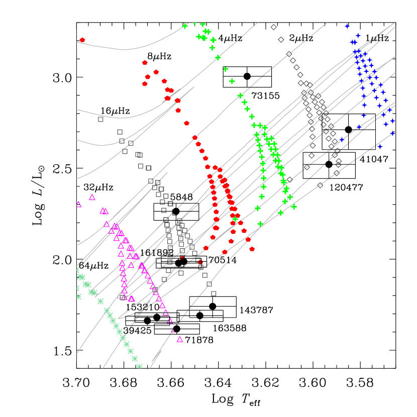
Figure 2.— H-R diagram of region around our target stars (solid dots inside $1\sigma$-error boxes). Gray lines are a representative sample of evolution tracks. The additional symbols show points along the evolution tracks corresponding to a given value of $\nu_{\mathrm{max}}$_,pre (values are indicated for each symbol).

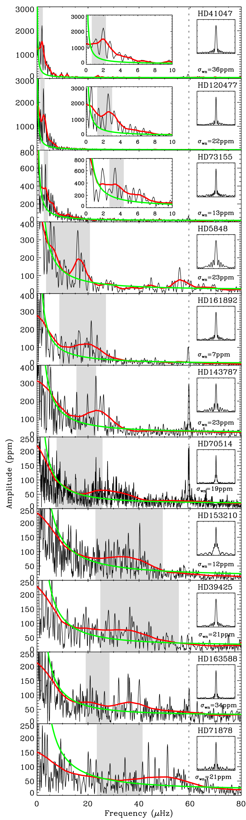
Figure 3.— Amplitude spectra of the 11 K giants (HD numbers are indicated). Note the increasing amplitude scale on the ordinate. In each panel the red solid line is a smoothed version of the spectrum and the green monotonically decreasing line is a fit to the noise. Gray shaded areas indicate the frequency interval of $\nu_{\mathrm{max}}$_,pre. The dotted line marks one third of the WIRE orbital frequency, and $\sigma_{\mathrm{wn}}$ is the square root of the mean power in the range: 70–80 $\mu$Hz. The inset is the spectral window in amplitude, shown in the same horizontal scale as the main panels.

References

- Alonso et al. (1999) Alonso, A., Arribas, S., & Martínez-Roger, C. 1999, A&AS, 140, 261
- Baglin & The COROT Team (1998) Baglin, A., & The COROT Team. 1998, in IAU Symp. 185: New Eyes to See Inside the Sun and Stars, Vol. 185, 301
- Barban et al. (2007) Barban, C., et al. 2007, A&A, 468, 1033
- Bedding & Kjeldsen (2003) Bedding, T. R., & Kjeldsen, H. 2003, PASA, 20, 203
- Blackwell & Lynas-Gray (1998) Blackwell, D. E., & Lynas-Gray, A. E. 1998, A&AS, 129, 505
- Brown et al. (1991) Brown, T. M., Gilliland, R. L., Noyes, R. W., & Ramsey, L. W. 1991, ApJ, 368, 599
- Bruntt et al. (2005) Bruntt, H., Kjeldsen, H., Buzasi, D. L., & Bedding, T. R. 2005, ApJ, 633, 440
- Christensen-Dalsgaard (2004) Christensen-Dalsgaard, J. 2004, Sol. Phys., 220, 137
- Christensen-Dalsgaard et al. (2007) Christensen-Dalsgaard, J., Arentoft, T., Brown, T. M., Gilliland, R. L., Kjeldsen, H., Borucki, W. J., & Koch, D. 2007, Comm. in Asteroseismology, 150, 350
- Cutri et al. (2003) Cutri, R. M., et al. 2003, 2MASS All Sky Catalog of point sources (Pasadena: NASA/IPAC)
- De Ridder et al. (2006) De Ridder, J., Barban, C., Carrier, F., Mazumdar, A., Eggenberger, P., Aerts, C., Deruyter, S., & Vanautgaerden, J. 2006, A&A, 448, 689
- di Benedetto (1998) di Benedetto, G. P. 1998, A&A, 339, 858
- Frandsen et al. (2002) Frandsen, S., et al. 2002, A&A, 394, L5
- Guenther et al. (2007) Guenther, D. B., et al. 2007, Comm. in Asteroseismology, 151, 5
- Hekker et al. (2006) Hekker, S., Reffert, S., Quirrenbach, A., Mitchell, D. S., Fischer, D. A., Marcy, G. W., & Butler, R. P. 2006, A&A, 454, 943
- Houdek & Gough (2002) Houdek, G., & Gough, D. O. 2002, MNRAS, 336, L65
- Kallinger et al. (2007) Kallinger, T., et al. 2007, preprint (astro-ph/0711.0837)
- Kjeldsen & Bedding (1995) Kjeldsen, H., & Bedding, T. R. 1995, A&A, 293, 87
- Kjeldsen et al. (2005) Kjeldsen, H., et al. 2005, ApJ, 635, 1281
- Kučinskas et al. (2005) Kučinskas, A., Hauschildt, P. H., Ludwig, H.-G., Brott, I., Vansevičius, V., Lindegren, L., Tanabé, T., & Allard, F. 2005, A&A, 442, 281
- McWilliam (1990) McWilliam, A. 1990, ApJS, 74, 1075
- Pietrinferni et al. (2004) Pietrinferni, A., Cassisi, S., Salaris, M., & Castelli, F. 2004, ApJ, 612, 168
- Stello et al. (2007) Stello, D., et al. 2007, MNRAS, 377, 584
- Stello et al. (2006) Stello, D., Kjeldsen, H., Bedding, T. R., & Buzasi, D. 2006, A&A, 448, 709
- Stello et al. (2004) Stello, D., Kjeldsen, H., Bedding, T. R., De Ridder, J., Aerts, C., Carrier, F., & Frandsen, S. 2004, Sol. Phys., 220, 207
- Tarrant et al. (2007) Tarrant, N. J., Chaplin, W. J., Elsworth, Y., Spreckley, S. A., & Stevens, I. R. 2007, MNRAS, 382, L48
- van Leeuwen (2007) van Leeuwen, F. 2007, Hipparcos, the New Reduction of the Raw Data, Astroph. and Sp. Sc. Lib., Vol. 350 (Springer Dordrecht)