Modeling a Maunder Minimum

Abstract

We introduce on/off intermittency into a mean field dynamo model by imposing stochastic fluctuations in either the alpha effect or through the inclusion of a fluctuating electromotive force. Sufficiently strong small scale fluctuations with time scales of the order of 0.3-3 years can produce long term variations in the system on time scales of the order of hundreds of years. However, global suppression of magnetic activity in both hemispheres at once was not observed. The variation of the magnetic field does not resemble that of the sunspot number, but is more reminiscent of the ¹⁰Be record. The interpretation of our results focuses attention on the connection between the level of magnetic activity and the sunspot number, an issue that must be elucidated if long term solar effects are to be well understood.

1 Introduction

The sun shows variability on a broad range of time scales, from milliseconds to millennia and on to even longer scales. Here we are interested in the time scales associated with the solar cycle and its grand minima. A salient manifestation of the cyclic behavior is seen in the sunspot number, whose annual mean oscillates on a scale of eleven years (or twenty-two years, if one goes by magnetic polarity variations). The term “cycle” is used to describe this oscillation in the sense that the sunspot number qualitatively performs the same kind of oscillation approximately every eleven years, with an amplitude that varies in a way that is reminiscent of some chaotic oscillators. However, it has been found that we do not have sufficient data to decide whether the global solar magnetic variation is chaotic, in the sense that its temporal behavior may be that of a low-order deterministic dynamical system (Spiegel & Wolf 1987). Nevertheless, a chaotic oscillator offers a natural way to model various irregularities of the solar cycle (Spiegel 1977; Tavakol 1978; Ruzmaikin 1981).

Like certain simple chaotic systems, the sun repeats itself magnetically over and over again, but never quite the same way twice, much in the manner of simple chaotic oscillators. On the other hand, the simplest chaotic dynamos (Allan 1962; Robbins 1979) do not exhibit the kind of strong intermittency such as was seen in the Maunder Minimum (Eddy 1978) when the amplitude of the oscillation in sunspot numbers went nearly to zero for seventy-five years in the time of Newton. This behavior is suggestive of the possibility that a strongly intermittent chaotic oscillator needs to be invoked in trying to understand the solar oscillation. Oscillators that behave this way are known (Spiegel 1981; Fautrelle & Childress 1982) but, when they are in the active phase, their variations do not normally resemble those of the sunspot number.

In modeling the solar magnetic variability with simple oscillators, it is not obvious how to connect the output of the models with the sunspot number. It may therefore not be damning if the variations produced by a model do not reproduce even qualitatively the variations seen in the sunspot number. Nevertheless, in terms of nonlinear lumped models, whose behavior is purely temporal, it has been possible to produce variations of the cyclic behavior that resemble those seen in the grand minima qualitatively either by modulation (Weiss et al. 1984) or intermittency (Platt et al. 1993b). But the solar variability is manifestly spatio-temporal and lumped models can at best provide clues to the actual processes involved in the solar cycle. Here we describe an attempt to go beyond models with purely temporal variations to models showing spatio-temporal variations that also produce analogues of the grand solar minima.

An earlier version of this paper was composed in the early nineties and some added remarks were inspired by discussions at the Enrico Fermi School in Varenna (Cini Castagnoli & Provenzale 1997). In the meantime a lot of new work has emerged, but we feel that the ideas presented here are still relevant. Particularly important has been the work of Beer et al. (1998) in demonstrating the persistence of a solar activity cycle throughout the time of the Maunder Minimum. Such behavior emerged from a purely temporal model (Pasquero 1996) as well as from a one-dimensional dynamo model (Tobias 1996) with small turbulent magnetic Prandtl number (so that the viscous diffusion timescale is much longer than that for magnetic diffusion time). Similar results — also for small turbulent magnetic Prandtl numbers — have been obtained for two-dimensional models by incorporating quenching in the $\Lambda$-effect that drives the differential rotation (Küker et al. 1999). Intermittent behavior in dynamo models has been studied further by Tworkowski et al. (1998) using time-dependent alpha-quenching, and by Charbonneau et al. (2005) using algebraic alpha-quenching. However, intermittency can equally well occur in stochastically forced models (e.g. John et al. 2002). In the following, we discuss the spatio-temporal variability of similarly forced dynamo models in two dimensions assuming axisymmetry.

2 Spatio-temporal variability

The spatio-temporal dynamics of the solar cycle as seen in spacetime diagrams like the Maunder butterfly diagram suggest that solitary waves may play an active part in the solar activity cycle (Proctor & Spiegel 1991). A nonlinear version of Parker’s (1955) dynamo waves (Worledge et al. 1997) or solitary waves arising from another overstability could be the mechanism of the drifting of the center of activity in latitude through the cycle. The finite width of the activity zone at any given time suggests that the waves in question are themselves confined or guided by a layer of some corresponding thickness. The picture that we adopt here is the now conventional one that the layer is the tachocline, though such a layer has been variously considered to lie deep in the convection zone (DeLuca 1986), just below it (Spiegel & Weiss 1980) or occupy the full convective zone (Brandenburg 2005). It might operate on the standard ingredients of a dynamo — differential rotation and cyclonic convection — from which we here make a model. Since we first wrote those lines, the layer has been well studied both observationally and theoretically (Hughes et al. 2006). It mediates the transition between the outer differentially rotating layers of the convection zone and the inner core with its nearly constant angular velocity. It has been renamed the tachocline (Spiegel & Zahn 1992) in keeping with its gain in respectability.

Here we use mean field theory (Moffatt 1978; Krause & Rädler 1980) with the effects of small scale motions subsumed into turbulent diffusivity and the $\alpha$-effect. Though mean field dynamos may not tell the whole story of the solar magnetic fluctuations (e.g. Hoyng 1987; 1988), they will suit our purpose of modeling the intermittency signaled by the Maunder Minimum. In modeling solar intermittency, we need to be aware that there are several forms of intermittency that have been isolated in dynamical systems theory. However, there is a particular one that models the solar grand minima quite well (Pasquero 1996) and that has come to be called on/off intermittency (Platt et al. 1993a; see also Spiegel 1994). [In fact, this form of intermittency was fashioned (Spiegel 1981) with grand minima in mind.]

On/off intermittency is like the intermittency detected in the output of a probe in a turbulent fluid registering abrupt changes as laminar and turbulent fluid regions flow past it. One may think of this as a series of bursts or chaotic relaxation oscillations. What characterizes models that have been made of this process (e.g. Spiegel 1981; Ott & Chen 1990; Pikovsky & Grassberger 1991) is that the (potentially) unstable oscillator performing the cycle is driven to instability through coupling to an aperiodic driver that is continuously chaotic or stochastic. The role of the driver is to move the system into and out of the unstable state. Observations of the bursts cannot readily distinguish the chaotic driver from a stochastic alternative which works equally well (von Hardenberg et al. 1997), and the number of degrees of freedom involved in such an object in the solar case will be hard to determine (but see Heagy et al. 1994). Fortunately, the qualitative features of the process do not depend sensitively on this difference, and we shall use a stochastic driver here. In our present considerations, the action of the driver is meant to model the influence of the convective solar dynamo and the on/off oscillator represents the tachocline. Here we introduce on/off intermittency into a working model of the solar cycle (Rüdiger & Brandenburg 1995) that has not previously produced grand minima. Modulational grand minima in dynamo models have been found by Tobias. In the case of a distributed dynamo (Brandenburg 2005), on/off behavior may similarly be produced.

The effects of stochastic noise on mean field $\alpha\Omega$ dynamos have been studied previously (Choudhuri 1992; Moss et al. 1992; Hoyng et al. 1994), mainly to model irregularities of the solar cycle on time scales comparable to the solar cycle itself or shorter. Moss et al. (1992) suggested that a modulation of the solar cycle on longer timescales of the order of centuries should also be possible. More recently, work along those lines (Schmitt et al. 1996) has introduced the on/off intermittency mechanism into a mean-field style of dynamo, as had been used already in a lumped model of the solar cycle (Platt et al. 1993b). The present paper is similarly based on a relatively realistic model of the solar dynamo in being spatio-temporal and into which we introduce the on/off intermittency mechanism.

The main difference between our work and that of Schmitt et al. is that we consider a standard $\alpha$-effect while they introduced a lower cutoff excluding field generation below a field strength of 1 kG at the base of the convection zone. This kind of filtering is analogous to Durney’s (1995) introduction of a critical field value in the tachocline above which a magnetic tube is ejected. This also produces grand minima in spatio-temporal models.

Another difference with the calculation of Schmitt et al. is that we consider the full sun whereas they studied only a single hemisphere and produced one-winged butterflies. This relates to another aspect of the problem that our model is intended to bring out. It is very difficult to have both hemispheres go completely inactive for appreciable times. The probability of a complete turnoff is exceedingly low and it seems unlikely that any propagative intermittency mechanism with retardation effects could turn off the magnetic activity globally in models with large spatial extent. The model described here does however produce lowered solar activity over large portions of its computational domain and therefore gives the kind of reduction in total overall activity that is consistent with what was seen in the Maunder Minimum.

The hemispheric asymmetry has been modeled by Knobloch et al. (1998; see also Weiss 1993) and this work is related to the problem of making an extended system demonstrate on/off intermittency. The problem has something in common with that involved in laying a rug. Once the rug is nailed down, if there is a bump somewhere, there seems to be no way to squeeze it out of existence. We have observed the same behavior with the dynamo model. If we produce a grand minimum locally somewhere in space, we find invariably that there is usually some excitation elsewhere. While we can get a whole hemisphere to be quiet at one time, the other one may still show activity. The output of the dynamo model is therefore somewhat like the sun in intermission — on the global scale there is usually some weak activity somewhere and it does have cycles. [Pasquero (1996) has shown how this may be achieved in the purely temporal oscillators as well.] As we have learned at the Fermi School on the Interaction of the Solar Cycle with Terrestrial Activity in June of 1996, certain terrestrial data have much more in common with the output of the dynamo models than the sunspot number. Moreover, some of these terrestrial data are very convincing proxy data for the solar activity (Beer et al. 1990; 1994; 1996; Solanki et al. 2004), while others may mimic the sunspot number. [There are also auroral indicators of solar activity recorded in classical antiquity (Stothers 1979, Solow 2005).] To a great extent, the issue is at heart one of knowing how to compare the output of dynamo models to the various measures of solar activity.

We describe next some particulars of the model itself, including the manner in which the fluctuations are introduced. Readers who are not interested in such detailed information should skip directly to Sect. 4 where we outline the main results. In these, we focus on models with a rather high noise level exceeding the electromotive force from the $\alpha$-effect by an order of magnitude since we expect the global convective dynamo action to be more vigorous than that of the tachocline.

3 The model

We use a mean-field model of the dynamo action in the tachocline (Rüdiger & Brandenburg 1995) with an anisotropic $\alpha$-effect and a turbulent magnetic diffusivity. Magnetic buoyancy is also included as it is in the more elaborate model of Jiang et al. (2007; see further references therein). The prescribed angular velocity is taken from the observational findings of helioseismology (Christensen-Dalsgaard & Schou 1988). To obtain a 22 yr magnetic cycle period, we introduce a scaling factor in the magnetic diffusivity of 0.5 and, to get a butterfly diagram with sufficient activity at low latitudes, we introduce a suitable latitude dependence in $\alpha$.

In the original model calculations, the value of $\alpha$ was typically set at a value approximately twenty times the critical value for instability. To produce on/off intermittency (Platt et al. 1993a), in the highly supercritical case, we would need very large fluctuations at that value. In this exploratory study, we prefer to operate at more modest parameter values to avoid the need for large fluctuations in the driver. Therefore we choose a slightly subcritical value of $\alpha$ and introduce only modest fluctuations in its magnitude so that the driver can move it into and out of the unstable state easily. For this purpose we introduce a scaling factor $c_{\alpha}$ in front of certain components of the $\alpha$-tensor (those components which result from the interaction of rotation and stratification). For details see the original discussion of the model (Rüdiger & Brandenburg 1995) where, with $c_{\alpha}$ = 1, the resulting toroidal magnetic field is a few kgauss and the poloidal field at the surface about 10 gauss. In the cases studied here, however, where the dynamo is just marginally excited, the generated magnetic field is weak, and could not explain the field strength observed in sunspots. This feature of the model can be corrected, as the work of Schmitt et al. (1996) shows.

We consider separately two kinds of fluctuation in the model: fluctuations in $\alpha$ or in an imposed electromotive force ${\vec{\cal E}}$ representing the effect of the fluctuations in the main solar dynamo. The latter is a more elementary process that does not rely much on dynamo theory. The picture here is that in the bulk of the convection zone a small scale dynamo operates (e.g. Meneguzzi & Pouquet 1989; Nordlund et al. 1992) producing a magnetic field that is highly variable in space and time as represented by ${\vec{\cal E}}$. In the bulk of the convection zone the fluctuations are immense, hence even spatial and temporal averages (${\vec{\cal E}}=\langle\bm{u}^{\prime}\times\bm{B}^{\prime}\rangle$) remain fluctuating, albeit on longer scales (Brandenburg et al. 2008). The angular brackets refer to ensemble averages in principle but, in practice, they are approximated by spatial and temporal coarse graining averages. The error resulting from this approximation is sometimes interpreted as a source of stochastic noise (Hoyng 1987; 1988; 1993; Moss et al. 1992; Brandenburg et al. 2008). As we have mentioned, there is ample reason for expecting fluctuations to appear in any realistic model.

We adopt white noise with vanishing mean value and a root mean square value of unity. The temporal power spectrum of the noise is flat for frequencies smaller than $2\pi/\tau$. The value of $\tau$ determines the time span over which long term variability of the resulting mean magnetic field is possible. The amplitude of the noise, $n_{\cal E}$, is measured in terms of the rms velocity of the turbulent motions and the local equipartition field strength. Whichever of the fluctuation mechanisms applies — in the emf or in the $\alpha$ effect — the procedure is similar. For the $\alpha$ case, for example, we add a fraction $n_{\alpha}$ of the noisy component to the original $\alpha$.

4 Results

4.1 Fluctuating $\alpha$-effect

To regulate the strength of the effect of noise, we introduce a factor $c_{\alpha}$ in front of the familiar $\alpha$ term, as described in Sect. 3. With everything else fixed, instability occurs when $c_{\alpha}$ exceeds the critical value $c_{\alpha}^{\rm(crit)}\approx 0.03$. We begin by adopting the subcritical value $c_{\alpha}=0.02$ and we adjust the fluctuations in $\alpha$ to have a time scale $\tau=3\,{\rm yr}$.

If the noise level, $n_{\alpha}$ , is too low, the magnetic field decays to zero, as it does when $n_{\alpha}$ = 0.02. Short noisy bursts in $\alpha$ are insufficient to bring the magnetic field to appreciable strength. On the other hand, if $n_{\alpha}$ is rather larger than this, the magnetic field is almost entirely dominated by the noise and cyclic behavior does not occur, except for irregular reversals on the timescale of centuries. Such a case is depicted in Fig. 1, where we show a color-coded representation of the toroidal magnetic field at the bottom of the convection zone as a function of time and latitude. In the following we refer to such representations as butterfly diagrams. A very similar result, with reversals on a long time scale, is found even when the non-random component of $\alpha$ is absent altogether provided there is global shear in the tachocline, as there is in accretion disks (Vishniac & Brandenburg 1997).

To get sufficiently large magnetic field strengths, we focus attention on models with $c_{\alpha}=1$. With $\tau=3\,{\rm yr}$ we find long term variability on a time scale of $200$–$500\,{\rm yr}$; see Fig. 2. We associate this variability with grand minima (and maxima) as discussed below in Sect. 5 although as noted already, there is never a complete turning off of the cycle at all locations at once.

Even if $\tau$ is decreased to a value of $0.3\,{\rm yr}$, say, long term variability still occurs, but individual cycles may vary significantly in amplitude as seen in Fig. 3. Such behavior is found only if the fluctuations of $\alpha$ are sufficiently larger than the average value; here a factor of five is needed. Individual fluctuations of $\alpha$ can still be much larger because we have assumed an exponential distribution for the probability density of $\alpha$ fluctuations.

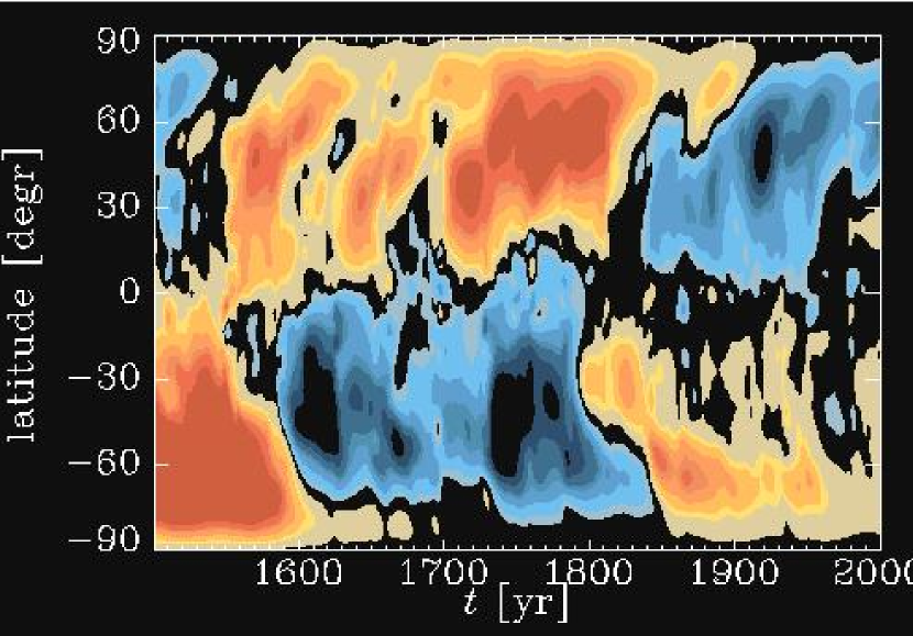
Figure 1: Butterfly diagrams of the toroidal field at the base of the convection zone for $c_{\alpha}=0.02$, $n_{\alpha}=5$ and $\tau=3\,{\rm yr}$.

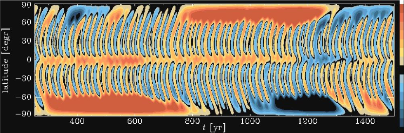
Figure 2: Butterfly diagrams of the toroidal field at the base of the convection zone for $c_{\alpha}=0.02$, $n_{\alpha}=5$ and $\tau=3\,{\rm yr}$. Butterfly diagrams of the toroidal field at the base of the convection zone for $c_{\alpha}$ = 1, $n_{\alpha}=0.2$ and $\tau=3\,{\rm yr}$.

4.2 Magnetic noise

If we introduce an external stochastic emf, as described in Sect. 3, we find a qualitatively similar behavior to that with fluctuating $\alpha$; see Fig. 4. Fluctuations of various kinds can evidently produce long time intermittency.

The model shows two distinct activity waves, one migrating equatorward and the other poleward. The two waves seem to be modulated independently, in each hemisphere. So do the modulations in the two hemispheres seem to be only weakly coupled, with little tendency to form a dipole structure. It may be that the approximate antisymmetry of the toroidal magnetic field of the sun, suggested by Hale’s polarity law, may not be a very stable feature, and that other types of (a)symmetry might have occurred in the past. Other, more regular parity variations of the magnetic field have previously been seen in nonlinear models (Brandenburg et al. 1989a,b; 1990; Jennings & Weiss 1991; Sokoloff & Nesme-Ribes 1994).

5 Interpretation

In the model described here, the seat of the solar activity cycle is in the solar tachocline, the layer that matches the differential rotation of the solar convection zone to the (nearly) rigid rotation of the inner sun (Hughes et al. 2006). While the precise hydromagnetic process that drives the activity has not yet been securely identified, we have assumed that the process may be modeled as an $\alpha\omega$ dynamo for the purpose of exploring the cause of the grand minima of solar activity. However, as we have already implied, any of several overstabilities might equally serve our purposes.

As we have tacitly assumed, the differential rotation in the tachocline is likely to be significant in such instabilities. In particular it is likely to give rise to a toroidal field. Given a suitable depth dependence of the strength of this field, an instability driven by magnetic buoyancy (Parker 1979) may arise and, especially in the presence of a stable density stratification, it may drive waves of excitation (Proctor & Spiegel 1991). Another possible driver for such waves may be magnetorotational instability (Balbus & Hawley 1998). Parfrey & Menou (2007) have studied the local instability of the tachocline and found instability at high latitudes and stability at low latitudes. However, their calculation did not include a toroidal field and, as Knobloch (1992) has observed, an azimuthal field can cause a Hopf bifurcation in MRI. As we may reasonably expect to find a toroidal field in the tachocline, this overstability is another mechanism that could perhaps engender waves whose description would typically be by the complex Ginzburg-Landau equation (Aranson & Kramer 2002). A related calculation is described by Kitchatinov and Rüdiger (2007); see also Cally (2003), Gilman et al. (2007), Rüdiger & Kitchatinov (2007), and Zahn et al. (2007).

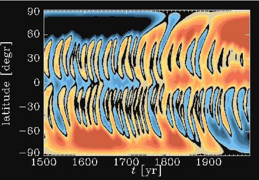
Figure 3: Butterfly diagrams of the toroidal field at the base of the convection zone for $c_{\alpha}=1$, $n_{\alpha}=5$ and $\tau=0.3\,{\rm yr}$.

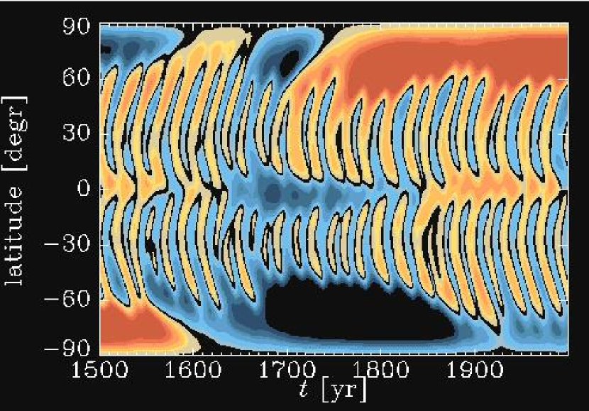
Figure 4: Butterfly diagrams of the toroidal field at the base of the convection zone for $c_{\alpha}=1$, $n_{\cal E}=1$ and $\tau=3\,{\rm yr}$.

Given that the tachocline is poised to drive hydromagnetic activity, by dynamo processes or otherwise, we have also assumed that the ambience is highly fluctuating. Here we have in mind that the main dynamo in the sun is a global convective dynamo. It is this process that is presumably responsible for the magnetic carpet (Simon et al. 2001) in a continuous process that is thought to produce rapidly fluctuating fields of moderate strength (Priest et al. 2002). In view of the complications in the theory of this process, we have simply modeled the highly fluctuating fields in of the solar convection zone as a stochastic process. In the mechanism of on/off intermittency that we have introduced here, the fluctuations produced by the main dynamo move the tachocline into and out of states of instantaneous overstability. This mechanism produces, as we have noted, longer response times in the model tachocline than the time scales of the fluctuations that give rise to more intense field concentrations. [We have seen a similar kind of symbiosis in the simulations of the geodynamo by Glatzmaier & Roberts (1995)]. The details of the process are complicated but, in gross, when the local field fluctuations produced are too weak, the grouping of flux ropes into a sunspot field is not achieved, even though much of the normal activity continues in the convection zone. To illustrate how such details may relate to the observed spot numbers, we have mapped the activity to the butterfly diagram with a particular functional of the field in the tachocline for the present purposes.

Like the sun, the model we have studied here manifests spatio-temporal intermittency but the magnetic activity almost never turns off everywhere. That is, our results suggest that simple dynamo models, with either fluctuating emfs and/or with magnetic noise injected into the bulk of the convection zone, can produce intermittency on sufficiently long time scales, but they do not switch off globally over the whole sun, in both hemispheres at once. It seems likely that this feature is inherent in all models with propagative behavior and that it cannot be expected that the cycle-producing processes of the sun switches off everywhere for several cycles as might be imagined on the basis of certain lumped models (such as Platt et al. 1993b). When we first produced the present results, we thought this feature was a deficiency. But as Ribes & Nesme-Ribes (1993) have reported, even during the Maunder Minimum, a weak solar cycle continued. Thus a globally depleted activity level is more like what is wanted and we have gotten that from the model in keeping with the historical records as interpreted by Ribes and Nesme-Ribes.

There still remains the need for an additional physical feature that relates to the production of sunspots, or more specifically, strong flux tubes of sufficiently large cross-section. That is the message of the procedures of Durney (1995) and Schmitt et al. (1996). A simple way of formulating this problem is to say that the sunspot number, which is a global parameter, is, as already mentioned, a functional of the various fields produced in the model. To get that functional, we need to operate with an explicit sunspot production mechanism.

Let $R(t)$ be the average magnetic field strength between $\pm 10^{\circ}$ and $\pm 30^{\circ}$ latitude, but allow only those areas where the field exceeds the root mean square value by 30 percent to contribute to this average. This quantity is plotted in Fig. 5. Note that $R(t)$ shows periods with almost vanishing magnetic activity as in a Maunder Minimum. The grand minima on this interpretation of the output of the models result from what may be regarded as lean cycles magnetically. If there are magnetic droughts, they are only local, not global, though the magnetic means may be low. In that sense, the sunspot number, though valuable for having focused our attention on an interesting feature of the magnetodynamics, may in some ways be a misleading indicator of what is happening overall.

Figure 5: Time series of $|B|$ (dotted line) and the activity parameter $R$ (solid line) for the same run as in Fig. 2. Note that the scale for $|B|$ increases downwards, in order to mimic the approximate anticorrelation between the ¹⁰Be data and the sunspot number.

This view is supported by studies of other indicators of solar activity than the sunspot number. The most complete records of variations that may result from solar activity fluctuations are found in the ¹⁰Be records from ice cores (Beer et al. 1990; 1994; 1996). The ¹⁰Be variations are plausibly attributed to modulation of the cosmic ray flux by the magnetic field in the solar wind (Beer et al. 1996). In Fig. 6 we reproduce data kindly provided by Dr. Jürg Beer comparing the ¹⁰Be records with the sunspot number for nearly four centuries. We see that a cyclic modulation is very much in evidence during the Maunder Minimum, with a rather modest reduction in its amplitude compared to that of the sunspot number.

Figure 6: ¹⁰Be data (solid line) together with the sunspot number (dotted line), as provided by Dr. Jürg Beer. The data are from a shallow core (300 m) drilled at Dye 3, Greenland, in 1986. The data were filtered using a spectral filter with a cut-off of 6 years and interpolated using a cubic spline. The younger part (1783-1985) is published in (Beer et al. 1990), and the whole record appeared in Beer et al. (1994).

The situation as brought out in the cited papers of Beer et al. is that various measures of solar activity are not perfectly correlated. If we were to think of the output of a model solar dynamo as we would one of these other measures, we would not be surprised that it does not necessarily represent all of them faithfully. Unfortunately, there is as yet no clear theoretical indication which one of them a model should most closely represent. If, in a grand minimum, there is high magnetic activity in only one hemisphere, it is not unreasonable that the modulations of ¹⁰Be should continue with reasonable strength. The question for the theory then is what is the relationship between the variations produced by the models and (say) the sunspot number. This is particularly difficult since the sunspots seem to be produced well within the sun and not at the surface, whereas some of the other activity measures are no doubt superficially produced. Even if we do have a good model of the cyclic mechanism, we also need to understand how sunspots form and surface before we can predict their number.

Nor is it unimportant to try to predict the sunspot number, or something akin to it, for it is this quantity that seems to be connected to some climatological variations. The most striking evidence of this is the discovery in tree ring data (Douglass 1927) that “the sunspot curve flattens out in a striking manner … from 1670 or 1680 to 1727.” This discovery was made by A.E. Douglas before he had “received a letter from Professor E. Maunder … calling attention to the prolonged dearth of sunspots between 1645 and 1715.” As Douglass and others have argued, variations in tree ring thickness in turn are connected to rainfall, so it is not an idle project to try to understand how to go from the workings of a solar dynamo to the manufacture of sunspots.

In summary, solar activity waves at high and low latitudes and in the two hemispheres, lead somewhat independent, weakly correlated lives and fluctuate separately under the influence of noise. Spatial variations of the solar cycle during the Maunder Minimum are not an immediate indicator of the sunspot number and, if the sunspots have their origin well beneath the solar surface, we must go another step in the discussion before we obtain results that are fully consistent with historic records of sunspots as summarized by Ribes and Nesme-Ribes (1993). It is not at all obvious what we may conclude about subconvective activity from observed surface activity.

- [1] Allan, D.W.: 1962, Proc. Camb. Phil. Soc. 58, 671
- [2] Aranson, I.S., Kramer, L.: 2002, Rev. Mod. Phys., 74, 99
- [3] Balbus, S.A., Hawley, J.F.: 1998, ReMP 70, 1
- [4] Beer, J., Blinov, A., Bonani, G., Hofmann, H.J., Finkel, R.C.: 1990, Nat 347, 164
- [5] Beer, J., Joos, F., Lukasczyk, Ch., Mende, W., Rodriguez, J., Siegenthaler, U., Stellmacher, R.: 1994, in: E. Nesme-Ribes (ed.), The Solar Engine and Its Influence on Terrestrial Atmosphere and Climate, Springer-Verlag Berlin Heidelberg, p. 221
- [6] Beer, J., Mende, W., Stellmacher, R. White, O.R.: 1996, in: P.D. Jones, R.S. Bradley, J. Jouzel (eds.), Climatic Variations and Forcing Mechanisms for the Last 2000 Years, Springer -Verlag, Berlin Heidelberg, p. 501
- [7] Beer, J., Tobias, S., Weiss, N.: 1998, SoPh 181, 237
- [8] Brandenburg, A.: 2005, ApJ 625, 539
- [9] Brandenburg, A., Krause, F., Meinel, R., Moss, D., Tuominen, I.: 1989a, A&A 213, 411
- [10] Brandenburg, A., Krause, F., Tuominen, I.: 1989b, in: M. Meneguzzi, A. Pouquet, P.L. Sulem (eds.), Turbulence and Nonlinear Dynamics in MHD Flows Elsevier Science Publ. B.V., North-Holland, p. 35
- [11] Brandenburg, A., Meinel, R., Moss, D., Tuominen, I.: 1990, in: J.O. Stenflo (ed.), Solar Photosphere: Structure, Convection and Magnetic Fields, Kluwer Acad. Publ., Dordrecht, p. 379
- [12] Brandenburg, A., Rädler, K.-H., Rheinhardt, M., Käpylä, P. J.: 2008, ApJ 676, arXiv: 0710.4059
- [13] Cally, P.S.: 2003, MNRAS 339, 957
- [14] Charbonneau, P., St-Jean, C., Zacharias, P.: 2005, ApJ 619, 613
- [15] Choudhuri, A.R.: 1992, A&A 253, 277
- [16] Christensen-Dalsgaard, J., Schou, J.: 1988, in: E.J. Rolfe (ed.), Proc. Symp. Seismology of the Sun and Sun-like Stars, ESA SP-286, p. 149
- [17] Cini Castagnoli, G., Provenzale, A. (Eds.): 1997, Past and Present variability of the solar-terrestrial system: Measurement, Data Analysis and Theoretical Models, (IOS Press, Amsterdam), 311
- [18] DeLuca, E. E.: 1986, Dynamo theory for the interface between the Convection Zone and the Radiative Interior of a Star, Thesis, U. Colorado, NCARCT-104
- [19] Douglass, A.E.: 1927, Sci LXV, 220
- [20] Durney, B.R.: 1995, SoPh 166, 231
- [21] Eddy, J.A.: 1978, in: J.A. Eddy (ed.), The New Solar Physics, AAAS Selected Symposium 17, Westview Press, Boulder, Colorado, p. 11
- [22] Fautrelle, Y., Childress, C.: 1982, GApFD 22, 235
- [23] Gilman, P.A., Dikpati, M., Miesch, M.S.: 2007, ApJS 170, 203
- [24] Glatzmaier, G.A., Roberts, P.H.: 1995, Nat 377, 203
- [25] Heagy, J.F., Platt, N., Hammel, S.M.: 1994, PhRvE 49, 1140
- [26] Hughes, D. W., Rosner, R., Weiss, N. O.: 2006, The Solar Tachocline, Cambridge University Press, Cambridge
- [27] Jennings, R., Weiss, N.O.: 1991, MNRAS 252, 249
- [28] Jiang, J., Chatterjee, P., Choudhuri, A.R.: 2007, MNRAS, 381, 1527
- [29] John, T., Behn, U., Stannarius, R.: 2002, PhRvE 65, 046229
- [30] Hoyng, P.: 1987, A&A 171, 357
- [31] Hoyng, P.: 1988, ApJ 332, 857
- [32] Hoyng, P.: 1993, A&A 272, 321
- [33] Hoyng, P., Schmitt, D., Teuben, L. J. W.: 1994, A&A 289, 265
- [34] Kitchatinov, L.L., Rüdiger, G.: 2007, Astron. Nachr. 328, 1150
- [35] Krause, F., Rädler, K.-H.: 1980, Mean Field Magnetohydrodynamics and Dynamo Theory, Akademie-Verlag, Berlin; also Pergamon Press, Oxford
- [36] Knobloch, E.: 1992, MNRAS 255, 25
- [37] Knobloch, E., Tobias, S.M., Weiss, N.O.: 1998, MNRAS 297, 1123
- [38] Küker, M., Arlt, R., Rüdiger, G.: 1999, A&A 343, 977
- [39] Meneguzzi, M., Pouquet, A.: 1989, JFM 205, 297
- [40] Moffatt, H. K.: 1978, Magnetic Field Generation in Electrically Conducting Fluids, Cambridge University Press, Cambridge
- [41] Moss, D., Brandenburg, A., Tavakol, R.K., Tuominen, I.: 1992, A&A 265, 843
- [42] Nordlund, Å., Brandenburg, A., Jennings, R.L., Rieutord, M., Ruokolainen, J., Stein, R.F., Tuominen, I.: 1992, ApJ 392, 647
- [43] Ott, E., Chen, Q.: 1990, PhRvL 65, 2935
- [44] Parfrey, K. P., Menou, K.: 2007, ApJ 667, L207
- [45] Parker, E. N.: 1955, ApJ 121, 293
- [46] Parker, E. N.: 1979, Cosmical Magnetic Fields: Their Origin and their Activity, (International Monographs on Physics)
- [47] Pasquero, C.: 1996, Model li di variabilit‘a solare, Tesi di Laurea, Facultà di Scienza M.F.N., Università di Torino
- [48] Pikovsky, A.S., Grassberger, P.: 1991, J. Phys. A 24, 4587
- [49] Platt, N., Spiegel, E.A., Tresser, C.: 1993a, PhRvL 70, 279
- [50] Platt, N., Spiegel, E.A., Tresser, C.: 1993b, GApFD 73, 146
- [51] Priest, E.R., Heyvaerts, J.F., Title, A.M.: 2002, ApJ 576, 533
- [52] Proctor, M. R. E., Spiegel E. A.: 1991, in: D. Moss, G. Rüdiger, I. Tuominen (eds), The Sun and Cool Stars, Springer-Verlag, p. 117
- [53] Ribes, J.C., Nesme-Ribes, E.: 1993, A&A 276, 549
- [54] Robbins, K. A.: 1979, SIAM J. Applied Math. 36, 457
- [55] Rüdiger, G., Brandenburg, A.: 1995, A&A 296, 557
- [56] Rüdiger, G., Kitchatinov, L.L.: 2007, NJPh 9, 302
- [57] Ruzmaikin, A. A.: 1981, Comments Astrophys. 9, 85
- [58] Schmitt, D., Schüssler, M., Ferriz-Mas, A.: 1996, A&A 311, L1
- [59] Simon, G.W., Title, A.M., Weiss, N.O.: 2001, ApJ 561, 427
- [60] Sokoloff, D.D., Nesme-Ribes, E.: 1994, A&A 288, 293
- [61] Solanki, S. K., Usoskin, I. G., Kromer, B., Schüssler, M., Beer, J.; 2004, Nat 431, 1084
- [62] Spiegel, E.A.: 1977, in: E.A. Spiegel, J.-P. Zahn (eds.), Problems in Stellar Convection, Springer-Verlag, Berlin Heidelberg, New York, p. 1
- [63] Spiegel, E.A.: 1981, in: R.H.G. Helleman (ed.), Nonlinear Dynamics, Ann. N.Y. Acad. Sci., 357, p.305
- [64] Spiegel, E.A.: 1994, in: M.R.E. Proctor, A.D. Gilbert (eds.), Lectures on Solar and Planetary Dynamos: Introductory Lectures, Cambridge University Press, Cambridge, p. 245
- [65] Spiegel, E.A., Weiss, N.O.: 1980, Nat 287, 616
- [66] Spiegel, E.A., Wolf, A.N.: 1987, in: J.R. Buchler, H. Eichhorn (eds.), Chaotic Phenomena in Astrophysics, Ann. N.Y. Acad. Sci., 497, p. 55
- [67] Spiegel, E.A., Zahn, J.-P.: 1992, A&A, 265, 106
- [68] Solow, A.R.: 2005, EPSL 232, 67
- [69] Stothers, R.: 1979, A&A 77, 121
- [70] Tavakol, R.K.: 1978, Nat 276, 802
- [71] Tobias, S.M.: 1996, A&A 307, L21
- [72] Tworkowski, A., Tavakol, R., Brandenburg, A., Brooke, J.M., Moss, D., Tuominen, I.: 1998, MNRAS 296, 287
- [73] Vishniac, E.T., Brandenburg, A.: 1997, ApJ 475, 263
- [74] von Hardenberg, J. Graf, Paparella, F., Platt, N., Provenzale, A., Spiegel, E.A., Tresser, C.: 1997, PhRvE 55, 58
- [75] Weiss, N.O., Cattaneo, F., Jones, C.A.: 1984, GApFD 30, 305
- [76] Weiss, N.O.: 1993, in: F. Krause, K.-H. Rädler, G. Rüdiger (eds.), The Cosmic Dynamo, Kluwer Acad. Publ., Dordrecht, p. 219
- [77] Worledge, D., Knobloch, E., Tobias, S., Proctor, M.: 1997, RSPSA 453, 119
- [78] Zahn, J.-P., Brun, A.S., Mathis, S.: 2007, A&A 474, 145
- [79]