We demonstrate that, in an appropriate limit, the off-shell M5-brane worldvolume action effectively captures the scalar potential of Seiberg-Witten theory perturbed by a small superpotential and, consequently, any nonsupersymmetric vacua that it describes. This happens in a similar manner to the emergence from M5’s of the scalar potential describing certain type IIB flux configurations [1]. We then construct exact nonholomorphic M5 configurations in the special case of $SU(2)$ Seiberg-Witten theory deformed by a degree six superpotential which correspond to the recently discovered metastable vacua of Ooguri, Ookouchi, Park [2], and Pastras [3]. These solutions take the approximate form of a holomorphic Seiberg-Witten geometry with harmonic embedding along a transverse direction and allow us to obtain geometric intuition for local stability of the gauge theory vacua. As usual, dynamical processes in the gauge theory, such as the decay of nonsupersymmetric vacua, take on a different character in the M5 description which, due to issues of boundary conditions, typically involves runaway behavior in MQCD.

1 Introduction

String theory has a rich history of providing geometric intuition for the structures that appear in supersymmetric field theories. For example, $NS5/D4$ constructions in type IIA and their corresponding $M$-theory lifts naturally give rise to the Riemann surfaces [4, 5, 6] which play such a crucial role on the gauge theory side [7, 8]. In this manner, the relation of geometry to the structure and properties of supersymmetric vacua is made completely manifest.

Since the recent discovery [9] that supersymmetric gauge theories often admit metastable SUSY-breaking vacua, significant effort has been devoted to the study of their stringy realizations [10, 11, 12, 13, 14, 15, 16, 17, 18, 19, 20, 21, 22, 23, 24, 25, 26, 27, 1, 28, 29, 30, 31, 32, 33, 34, 35, 36, 37, 38, 39, 40]. This is of particular interest for two reasons. First, one might hope to learn about the role played by geometry in the structure of nonsupersymmetric vacua in gauge theory. Second, stringy embeddings of metastable vacua can potentially provide new means by which SUSY-breaking can be achieved in string theory. Such constructions are typically local in nature and are thus well-suited to the sort of stringy model building advocated in [41].

One potential pitfall is that classical brane constructions in type IIA and their $M$-theory lifts can be well-studied only in parameter regimes that are far from those in which the corresponding gauge theory description is valid. As such, there is no guarantee at the outset that string theory knows anything about physics away from supersymmetric vacua, where quantities are protected. Despite this fact, considerable progress has been made along this direction in the case of the ISS vacua of ${\cal{N}}=1$ SQCD [9] and a number of generalizations [13, 14, 15, 19, 22, 23, 29, 37, 38, 40], and it has been demonstrated that type IIA/M-theory realizations provide valuable intuition for the metastability of those vacua.

In this paper, we shall focus instead on the stringy realization of Seiberg-Witten theory deformed by a superpotential. Because one can tune the degree to which ${\cal{N}}=2$ SUSY is broken, the Kähler potential is under some degree of control. This not only allows one to reliably compute the scalar potential in the gauge theory, it also gives us hope that the standard stringy realizations might allow us to engineer the full potential, in a suitable sense, along with any non-SUSY vacua that it describes.

As is well-known by now, deformed Seiberg-Witten theory admits two possible low energy descriptions depending on the various scales involved in the problem. If the characteristic scale, $g$, of the superpotential that controls the mass of the adjoint scalar is sufficiently small compared to the dynamical scale, $\Lambda$, of the gauge group, then the superpotential only plays a role in the deep IR after one has moved to the effective Abelian theory on the Coulomb branch. This is the situation referred to above in which the Kähler potential is under tunably good control. On the other hand, if $g$ is much larger than $\Lambda$, we should integrate out the adjoint scalar before passing to the IR. The ${\cal{N}}=2$ SUSY is broken to ${\cal{N}}=1$ and the gauge group is Higgs’ed at a high scale, below which non-Abelian factors confine. Certain aspects of the low energy dynamics, such as chiral condensate and the value of superpotential in supersymmetric vacua, are captured by an effective theory for the corresponding glueball superfields $S_{i}\sim\frac{1}{32\pi^{2}}\text{tr}\,W_{\alpha\,i}^{2}$ [42, 43] and corrections from the massive adjoint scalar lead to generation of the Dijkgraaf-Vafa superpotential [44, 45, 46, 47].

As pointed out by [48] and [18] in the context of the type IIB realization of this story via large $N$ duality [49, 50, 51], the appearance of FI terms suggests that the glueball effective theory actually possesses a spontaneously broken ${\cal{N}}=2$ supersymmetry. This again gives one control over the Kähler potential and allows a scalar potential to be reliably computed. Quite remarkably, the IIA brane construction which realizes deformed Seiberg-Witten theory admits an $M$-theory lift that incorporates and unifies the scalar potentials of both regimes. In particular, each can be obtained from a different limit of the $M5$ worldvolume action and hence both follow from simple minimal area equations. That the Dijkgraaf-Vafa potential is accurately encoded was essentially derived in [1]. In this paper, we will explicitly demonstrate how the Seiberg-Witten potential can also be realized in a suitable limit .

As an application of this result, we then proceed to describe stringy embeddings of the metastable vacua of deformed Seiberg-Witten theory recently discovered by Ooguri, Ookouchi and Park [2] and Pastras [3], which we will refer to as OOPP vacua. More specifically, we will find exact minimal area M5’s which reduce in the appropriate limit to minima of the Seiberg-Witten potential. By taking a IIA limit of these configurations, we will also be able to obtain a simple geometric picture for these vacua analogous to that of [13, 14, 15] for the ISS vacua [9]. This will allow us to obtain a semiclassical understanding from the $NS5/D4$ point of view of the full scalar potential itself, as well as the stability of the supersymmetry-breaking vacua. To our knowledge, the resulting mechanism of SUSY-breaking in brane constructions is novel.

While this work was in progress, a different approach to the realization of OOPP vacua appeared [35] which incorporates the superpotential of [2, 3] in a slightly different manner. While it can be written in a single trace form, the superpotential of [2, 3] nonetheless has degree larger than the rank of the gauge group and hence can also be viewed as a multitrace object. The authors of [35] took this point of view and attempted to realize the OOPP theory by using extra NS5-branes to directly engineer a multitrace superpotential. We take a different approach motivated by the $T$-dual type IIB constructions where a single-trace superpotential determines the geometry and the rank of the gauge group simply specifies the number of $D5$ branes that can occupy singular points. From this point of view, the background geometry remains the same regardless of how many or how few $D5$ branes we wish to add. As such, we realize the OOPP superpotentials by simply curving the NS5-branes in the same manner that we would for an identical superpotential with gauge group of arbitrarily high rank. That we are able to obtain the Seiberg-Witten potential from the M5 worldvolume action in this way seems to justify the use of this approach for engineering aspects of the OOPP theory away from the supersymmetric vacua. It would be interesting to study whether this might also be possible in the setup of [35]

The organization of this paper is as follows. We begin in section 2 with a brief review of the type IIA/M construction of deformed Seiberg-Witten theory. In section 3, we then review the mechanism described in [1] by which this construction is able to realize not only the space of supersymmetric vacua, but also the full scalar potential for the light degrees of freedom in the Dijkgraaf-Vafa regime. We then perform a similar analysis in the Seiberg-Witten regime in section 4 to demonstrate that the IIA/M picture captures the scalar potential there as well. In section 5, we review the manner in which nonsupersymmetric vacua can be engineered in the Seiberg-Witten regime by choosing a suitable superpotential [2, 3]. In section 6, we specialize to the case of $SU(2)$ and construct exact minimal-area $M5$ configurations corresponding to these vacua. In section 7, we study their semiclassical limit and obtain a simple interpretation in the NS5/D4 language of the potential and mechanism by which stability is achieved. We close with some concluding remarks in section 8. The Appendices include various technical details that we use in the main text.

2 Type IIA/M Description of Deformed Seiberg-Witten Theory

Let us begin with a brief review of the type IIA/M realization of $SU(N)$ ${\cal{N}}=2$ supersymmetric Yang-Mills theory deformed by a superpotential for the adjoint scalar. As first shown by Witten [4], the theory without superpotential can be engineered in type IIA by starting with two NS5-branes and $N$ D4-branes extended along the 0123 directions. The NS5’s are further extended along a holomorphic direction parametrized by the combination

$$v=x^{4}+ix^{5}$$ (2.1)

and the D4’s are suspended between them along $x^{6}$ as depicted in figure -179(a). If we scale the NS5 separation $L$ along $x^{6}$ to zero, the D4 worldvolume becomes effectively four-dimensional with gauge coupling constant given by

$$\frac{8\pi^{2}}{g_{YM}^{2}}=\frac{L}{g_{s}\sqrt{\alpha^{\prime}}}.$$ (2.2)

The resulting configuration preserves 8 supercharges, so this worldvolume theory is nothing other than the celebrated ${\cal{N}}=2$ $SU(N)$ supersymmetric Yang-Mills theory studied by Seiberg and Witten [7].

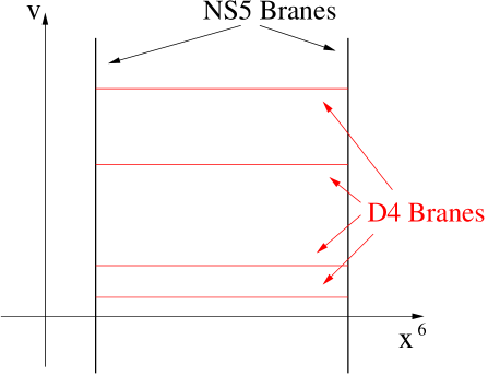
(a) NS5/D4 realization of the classical Seiberg-Witten moduli space.

(b) Cartoon of M5 lift which realizes the quantum Seiberg-Witten moduli space.

Figure -179: Type IIA/M realization of classical and quantum moduli space of Seiberg-Witten theory.

2.1 Classical and Quantum Moduli Space from Geometry

Because of the protection afforded by supersymmetry, we expect that the moduli space of vacua can be seen directly in the brane constructions, even away from the strict $L\rightarrow 0$ limit. In figure -179(a), for example, the classical moduli space of Seiberg-Witten theory is evident in our ability to place the D4’s at arbitrary values of $v$. To describe the quantum moduli space, however, it is necessary to accurately treat the NS5/D4 intersection points. While the strength of the string coupling in the NS5 throat makes this difficult to do directly in type IIA, Witten pointed out [4] that one can make progress by noting that NS5’s and D4’s are two different manifestations of the same object, namely the M5 brane of M-theory. As a result, the configuration of figure -179(a) should be replaced by a single M5 with four directions along 0123 and the remaining two, in the probe approximation, extended on a nontrivial two-dimensional surface $\Sigma$ of minimal area. From the IIA point of view, this will take the form of a curved NS5-brane with flux.

Figure -178: Sample parametrization of the M5 curve as double-cover of $v$-plane for the case $n=3$ with $\hat{A}$ and $\hat{B}$ cycles indicated.

The general structure of the M5 curve associated to figure -179(a) can be seen by observing that, roughly speaking, the stacks of D4-branes blow up into tubes as illustrated in figure -179(b). Consequently, a point on the classical moduli space where the D4’s form $n$ distinct stacks will correspond to a Riemann surface $\Sigma$ of genus $n-1$ with two punctures. A convenient parametrization of this surface is as a double-cover of the $v$-plane with $n$ cuts, as depicted in figure -178. Roughly speaking, we can think of each sheet as an NS5 and the cuts as the tubes associated to the D4’s. In this case, the full embedding is specified by providing the $v$-dependence of $x^{6}$ and $x^{10}$, which are naturally paired into the complex combination [4]

$$s=R_{10}^{-1}\left(x^{6}+ix^{10}\right),$$ (2.3)

where

$$R_{10}=g_{s}\sqrt{\alpha^{\prime}}$$ (2.4)

is the radius of the M-theory circle. We will set $\alpha^{\prime}=1$ henceforth.

The embedding relevant for figure -179(a) must be holomorphic due to the supersymmetry and is determined by imposing boundary conditions appropriate for the system at hand. In particular, we must fix the separation of the NS5’s at some cutoff scale $\Lambda_{0}$ and specify the number of D4’s in each stack. These conditions can be conveniently summarized in terms of constraints on the periods of the 1-form $ds$ around the $\hat{A}$ and $\hat{B}$ cycles of figure -178

$$\frac{1}{2\pi i}\oint_{\hat{A}_{j}}ds=N_{j}\qquad\text{and}\qquad\frac{1}{2\pi i}\oint_{\hat{B}_{j}}ds=-\alpha_{j}.$$ (2.5)

Here $N_{j}$ is the number of D4-branes in the $j$th stack and

$$\alpha_{j}=-\frac{4\pi i}{g_{YM}^{2}}+\frac{\theta_{j}}{2\pi}$$ (2.6)

with $g_{YM}^{2}$ denoting the bare coupling at scale $\Lambda_{0}$. In general, one can consider nontrivial relative $\theta_{j}$ angles by allowing the $\alpha_{j}$ to differ by integers. From this point onward, however, we shall restrict for simplicity to the case in which all $\alpha_{j}$ are equivalent:

$$\alpha_{j}\equiv\alpha\quad\text{for all }j.$$ (2.7)

To find the family of curves which satisfy the constraints (2.5) for various choices of $N_{j}$, Witten [4] noted that since the periods of $ds$ take integer values, the coordinate

$$t\equiv\Lambda^{N}e^{-s}$$ (2.8)

must be well-defined on the curve. With this observation, he demonstrated that the M5 lifts are described by nothing other than the Seiberg-Witten geometries

$$t^{2}-2P_{N}(v)t+\Lambda^{2N}=0,$$ (2.9)

where $P_{N}(v)$ is a polynomial of degree $N$ and

$$\Lambda^{2N}=\Lambda_{0}^{2N}e^{2\pi i\alpha}$$ (2.10)

is the dynamical scale of the gauge group. Generic choices of $P_{N}(v)$ lead to (degenerate) genus $N$ surfaces and hence correspond to lifts of classical configurations in which all $D4$-branes are separated. For special choices of $P_{N}(v)$, however, the curves (2.9) degenerate into surfaces of lower genus which describe the lifts of configurations with some $N_{j}>1$.

2.2 Turning on a Superpotential

To similarly engineer the ${\cal{N}}=2$ theory deformed by a polynomial superpotential $W_{n}(\Phi)$ of degree $n+1$, we need only modify the NS5/D4 construction of figure -179(a) by curving the NS5-branes appropriately [5, 53, 54]. More specifically, we introduce the complex combination

$$w=x^{7}+ix^{8}$$ (2.11)

and extend the NS5’s along the holomorphic curves $w(v)=\pm W_{n}^{\prime}(v)$. An example of such a configuration for the case of a cubic superpotential is depicted in figure -177. Classically, the supersymmetric vacua correspond to configurations where the D4-branes sit at zeros of $W_{n}^{\prime}(v)$, in accordance with our expectations from the gauge theory side.

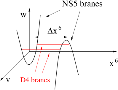
Figure -177: Sample NS5/D4 realization of supersymmetric vacua in $U(N)$ ${\cal{N}}=2$ supersymmetric Yang-Mills with a cubic superpotential.

At quantum level, the supersymmetric vacua are again effectively captured by moving to the M5 lift. The only new ingredient here is the addition of an extra nontrivial embedding coordinate whose $v$-dependence we must specify. The boundary conditions appropriate for that coordinate are determined by the asymptotic geometry of the NS5’s, meaning that we must impose

$$w(v)\sim\pm W_{n}^{\prime}(v)$$ (2.12)

near the points at infinity. Holomorphic solutions to this constraint take the form

$$w(v)=\sqrt{W_{n}^{\prime}(v)^{2}-f_{n-1}(v)}$$ (2.13)

for $f_{n-1}(v)$ a generic polynomial of degree $n-1$. If we further require consistency of the $w(v)$ and $s(v)$ embeddings, we are led to the factorization formulae

$$P_{N}(v)^{2}-4\Lambda^{2N}=S_{N-n}(v)^{2}\left(W_{n}^{\prime}(v)^{2}-f_{n-1}(v)\right)$$ (2.14)

if $n<N$ and similarly

$$\left(P_{N}(v)^{2}-4\Lambda^{2N}\right)H_{n-N}(v)^{2}=W_{n}^{\prime}(v)^{2}-f_{n-1}(v)$$ (2.15)

if $n>N$. For given $W_{n}^{\prime}(v)$, there are at most a finite number of choices for $P_{N}(v)$, $f_{n-1}(v)$, and $S_{N-n}(v)$ ($H_{n-N}(v)$), which satisfy (2.14) ((2.15)). This reflects the familiar fact that adding a superpotential to Seiberg-Witten theory lifts all but a discrete set of points on the moduli space. That these conditions yield vacua in agreement with the gauge theory analysis has been well-established [55, 56] and will also fall out naturally from our general formalism to follow.

3 The Dijkgraaf-Vafa Regime

We now turn to a study of physics away from the supersymmetric vacua. As discussed in the introduction, the appropriate IR description depends strongly on the relative sizes of the characteristic mass $g$ of the adjoint scalar field and the dynamical scale $\Lambda$. In this section, we consider the case where $g$ is sufficiently large compared to $\Lambda$.

3.1 Review of the Gauge Theory Side

On the gauge theory side, when $g$ is sufficiently large the gauge group is Higgs’ed and ${\cal{N}}=2$ supersymmetry broken to ${\cal{N}}=1$ at a high scale. The remaining non-Abelian factors confine and certain aspects of the IR dynamics can be captured by the glueball superfields $S^{i}=-\frac{1}{32\pi^{2}}\mathop{\mathrm{tr}}\nolimits W_{\alpha}^{i\,2}$ as well as the ${\cal{N}}=1$ gauge multiplets corresponding to the overall $U(1)$’s . The leading contribution to the glueball superpotential is given by the Veneziano-Yankielowicz term [42] and corrections arising from the presence of the adjoint scalar can be computed by integrating it out order by order in perturbation theory [47]. This calculation receives contributions only from planar diagrams which can in turn be computed with an auxiliary holomorphic matrix model

$$Z=\int\,{\cal{D}}\Phi\,\exp\left(-\frac{1}{g_{s}}\mathop{\mathrm{tr}}\nolimits W_{n}(\Phi)\right).$$ (3.1)

In the end, one arrives at the famous Dijkgraaf-Vafa superpotential [44, 45, 46]

$$W=\alpha_{i}S^{i}+N^{i}\frac{\partial{\cal{F}}}{\partial S^{i}}(S^{j}),$$ (3.2)

where $N^{i}$ denote ranks of the confining non-Abelian factors, $\alpha_{i}$ are as in (2.6) and ${\cal{F}}$ is the planar contribution to the free energy of (3.1) from the saddle point where $N^{i}$ eigenvalues of $\Phi$ sit at the $i$th critical point of $W_{n}(\Phi)$. Note that in writing ${\cal{F}}$ as a function of $S^{i}$, we must make the identification $S^{i}\sim g_{s}N^{i}$. This Dijkgraaf-Vafa superpotential was also derived from anomaly arguments in [43].

As usual, the matrix model computation can be reinterpreted in a geometric language based on the corresponding spectral curve. In the case at hand, this auxiliary Riemann surface takes the form

$$w^{2}=W_{n}^{\prime}(v)^{2}-f_{n-1}(v)$$ (3.3)

and the function ${\cal{F}}$ is simply its prepotential. To make this more precise, let us use the double-cover of the $v$-plane to parametrize (3.3) and specify $\hat{A}$ and $\hat{B}$ cycles as in figure -178. The quantities $S^{i}$ and $\partial{\cal{F}}/\partial S^{j}$ are then given by suitable $\hat{A}$ and $\hat{B}$ period integrals

$$S^{j}=\frac{1}{2\pi i}\oint_{\hat{A}_{j}}\,w\,dv\qquad\qquad\frac{\partial{\cal{F}}}{\partial S^{j}}=\frac{1}{2\pi i}\oint_{\hat{B}_{j}}\,w\,dv.$$ (3.4)

As usual, $\partial_{j}\partial_{k}{\cal{F}}\equiv\hat{\tau}_{jk}\,$ yields the period matrix of the Riemann surface (3.3).

These geometric formulae arise quite naturally when this theory is engineered in type IIB using $D5$-branes wrapping singular 2-cycles of a local Calabi-Yau [48, 49, 50, 51]. There, large $N$ duality relates the brane setup to a deformed Calabi-Yau with flux, whose superpotential takes the precise form (3.2). In this context, it has been conjectured that the IR physics contains an underlying ${\cal{N}}=2$ structure [48, 18], which gives one control over the Kähler metric. Such a possibility is suggested by the observation that the IR degrees of freedom naturally combine into $n$ ${\cal{N}}=2$ vector multiplets and the superpotential (3.2) is simply a linear combination of electric and magnetic Fayet-Iliopoulos parameters. If the conjecture is true, it would imply that we have some control over the Kähler metric and, in particular, that it can be identified with the imaginary part of the period matrix, $\mathop{\mathrm{Im}}\nolimits\hat{\tau}_{ij}$, of (3.3). In that case, the scalar potential takes a relatively simple form

$$V_{DV}=\overline{\left(\alpha_{i}+N^{k}\hat{\tau}_{ki}\right)}\left(\mathop{\mathrm{Im}}\nolimits\hat{\tau}\right)^{ij}\left(\alpha_{j}+\hat{\tau}_{j\ell}N^{\ell}\right).$$ (3.5)

In the next subsection, we will review the result of [1] that this potential is naturally encoded in the type IIA/M realization of the gauge theory. The resulting configuration is actually related to the IIB setup described above by a $T$-duality [58, 59]. Because the IIA/M and IIB descriptions are only reliable in widely-separated regions of parameter space, agreement of the scalar potentials was far from guaranteed and provides significant indirect evidence that, at least in the string picture, some residual ${\cal{N}}=2$ supersymmetry may be present.

3.2 Type IIA/M Description

From the point of view of our NS5/D4 constructions, the Dijkgraaf-Vafa regime has the natural interpretation as one where the D4’s are essentially pinned to the zeroes of $W_{n}^{\prime}(v)$. This means that the low energy modes involve not motion of the D4’s, but rather fluctuations in the size of the tubes into which they blow up in the M5 lift. In other words, this is a regime where the $w(v)$ part of the curve is essentially rigid while the $s(v)$ embedding can fluctuate.

Such a limit is in fact quite natural because the $s$ coordinate comes with a natural scale, namely the radius of the M-circle $R_{10}=g_{s}\sqrt{\alpha^{\prime}}$. If we take $R_{10}$ to be small, in which case our minimal area M5 instead has the interpretation of a curved NS5-brane with flux, we expect that variations of the $s$ coordinate of the embedding actually comprise the lightest excitations of the system. To make this more precise, let us introduce a “worldsheet” coordinate, $z$, to parametrize the nontrivial part of the M5 and define our embedding by the functions

$$s(z,\bar{z}),\quad v(z,\bar{z}),\quad w(z,\bar{z}).$$ (3.6)

In the probe approximation, the worldvolume theory is described by the Nambu-Goto action

$$S\sim\frac{1}{R_{10}^{2}}\int_{\Sigma}\,d^{2}z\,\sqrt{g(s,v,w)},$$ (3.7)

where $g(s,v,w)$ is the induced metric on the “worldsheet” $\Sigma$. If we suppose that $R_{10}ds\ll dw,dv$ then this action can be expanded to quadratic order as

$$S\sim\frac{1}{R_{10}^{2}}\int_{\Sigma}\,d^{2}z\,\sqrt{\tilde{g}(v,w)}+\int_{\Sigma}\,|ds|^{2}+\dots,$$ (3.8)

where $\tilde{g}(v,w)$ is the induced metric that arises from the $v$ and $w$ parts of the embedding alone. At small $R_{10}ds$, the dominant term of this action is the first one, whose equations of motion constrain the $w$ and $v$ coordinates to describe a minimal area embedding. If we further impose the holomorphic boundary conditions $w(v)\sim\pm W_{n}^{\prime}(v)$ near infinity, we are again led to the family of holomorphic curves

$$w^{2}=W_{n}^{\prime}(v)^{2}-f_{n-1}(v).$$ (3.9)

Note that the $\sqrt{\tilde{g}}$ term of (3.8) has flat directions corresponding to the complex moduli of (3.9).

Turning now to the second term of (3.7), the equations of motion for $ds$ imply that it must be a harmonic 1-form on (3.9). Because we fix the $\hat{A}$ and $\hat{B}$ periods of $ds$ according to (2.5), though, this leads to a unique $ds$ for each curve of the family (3.9). In particular, the 1-form $ds$ that we obtain exhibits explicit dependence on the complex moduli of (3.9) and hence, plugging this result back into the action, we find that $\int_{\Sigma}\,|ds|^{2}$ serves as a potential on the space of complex structures. It is precisely this object that will correspond to the scalar potential (3.5).

3.2.1 Regularization of the Action

Our M5’s are noncompact, though, so computations of their area must be carefully regulated. While we can do this quite easily by introducing a cutoff $\Lambda_{0}$ along $v$, it is important to make sure that this procedure leads to a result that is meaningful. The issue of computing regulated areas in this context has been discussed previously by de Boer et al. [60]. Our situation is essentially the same as theirs because, in the regime under consideration, the off-diagonal components of the induced metric $\tilde{g}(v,w)$ are negligible. Let us proceed to review their result, focusing for now only on the evaluation of $\int_{\Sigma}^{\Lambda_{0}}\,|ds|^{2}$.

Because $ds$ is harmonic, it can be written as the sum of a holomorphic 1-form $ds_{H}$ and an antiholomorphic 1-form $d\bar{s}_{A}$

$$ds=ds_{H}+d\bar{s}_{A}.$$ (3.10)

In this language, the object we want to compute is

$$\begin{split}\int_{\Sigma}^{\Lambda_{0}}\,|ds|^{2}&=\frac{1}{2i}\int_{\Sigma}^{\Lambda_{0}}\,\left[ds_{H}\wedge d\bar{s}_{H}+ds_{A}\wedge d\bar{s}_{A}\right]\\ &=\frac{1}{2i}\int_{\Sigma}^{\Lambda_{0}}\,\left[\left(ds_{H}\wedge d\bar{s}_{H}-ds_{A}\wedge d\bar{s}_{A}\right)+2ds_{A}\wedge d\bar{s}_{A}\right]\\ &=\frac{1}{2i}\int_{\Sigma}^{\Lambda_{0}}\,\left[ds\wedge d\bar{s}+2ds_{A}\wedge d\bar{s}_{A}\right].\end{split}$$ (3.11)

We have chosen to write it in this manner because $ds\wedge d\bar{s}$ is the restriction to $\Sigma$ of a closed 2-form in the target space. For this reason, its integral over $\Sigma$ should in fact be independent of the moduli. In practice, however, the regulated integral of $ds\wedge d\bar{s}$ will depend on both the moduli and the cutoff, $\Lambda_{0}$. Consequently, to obtain a meaningful regularization, we must choose the cutoff $\Lambda_{0}$ to vary with the moduli in such a manner that the regulated quantity

$$\frac{1}{2i}\int_{\Sigma}^{\Lambda_{0}}\,ds\wedge d\bar{s}$$ (3.12)

is indeed constant on the moduli space.

With such a scheme in place, the potential $\int_{\Sigma}^{\Lambda_{0}}\,|ds|^{2}$ is simply given by

$$\int_{\Sigma}^{\Lambda_{0}}\,|ds|^{2}\sim\frac{1}{i}\int_{\Sigma}^{\Lambda_{0}}\,ds_{A}\wedge d\bar{s}_{A},$$ (3.13)

where we have simply dropped the constant term (3.12). In the work of de Boer et al., the quantity analogous to (3.13) was cutoff-independent so this was the end of the story. In our case, however, this result may still exhibit a nontrivial dependence on the cutoff. Nevertheless, (3.13) provides a suitable notion of regularized area provided we also include the necessary moduli-dependence of $\Lambda_{0}$.

3.2.2 Evaluation of the Regulated $\int^{\Lambda_{0}}_{\Sigma}\,|ds|^{2}$

Let us turn now to evaluation of (3.13). We begin by using the constraint (2.5) to obtain an expression for $ds$ in terms of the period matrix $\hat{\tau}_{ij}$ of (3.9). We write $ds_{H}$ and $ds_{A}$ as

$$ds_{H}=h^{i}d\hat{\omega}_{i}\qquad\text{and}\qquad ds_{A}=\ell^{i}d\hat{\omega}_{i},$$ (3.14)

where the $d\hat{\omega}_{i}$ comprise a basis of $n$ holomorphic 1-forms, satisfying

$$\frac{1}{2\pi i}\oint_{\hat{A}_{j}}\,d\hat{\omega}_{i}=\delta_{ij}.$$ (3.15)

The $\hat{B}$-periods of $d\hat{\omega}_{i}$ yield elements of the period matrix

$$\frac{1}{2\pi i}\oint_{\hat{B}_{j}}\,d\hat{\omega}_{i}=\hat{\tau}_{ij}$$ (3.16)

and the constraints (2.5) become

$$\begin{split}h^{i}-\bar{\ell}^{i}&=N^{i},\\ h^{i}\hat{\tau}_{ij}-\bar{\ell}^{i}\bar{\hat{\tau}}_{ij}&=-\alpha_{j}.\end{split}$$ (3.17)

This implies that

$$\begin{split}h^{i}&=-\frac{1}{2i}\left(\mathop{\mathrm{Im}}\nolimits\hat{\tau}^{-1}\right)^{ij}\left(\alpha_{j}+\bar{\hat{\tau}}_{jk}N^{k}\right),\\ \bar{\ell}^{i}&=-\frac{1}{2i}\left(\mathop{\mathrm{Im}}\nolimits\hat{\tau}^{-1}\right)^{ij}\left(\alpha_{j}+\hat{\tau}_{jk}N^{k}\right).\end{split}$$ (3.18)

Now that we have determined $ds$, it is easy to evaluate

$$\begin{split}\frac{1}{i}\int_{\Sigma}\,ds_{A}\wedge d\bar{s}_{A}&=-2\mathop{\mathrm{Im}}\nolimits\left(\sum_{j}\oint_{\hat{A}_{j}}ds_{A}\,\oint_{\hat{B}_{j}}d\bar{s}_{A}\right)\\ &=8\pi^{2}\ell^{i}\left(\mathop{\mathrm{Im}}\nolimits\hat{\tau}\right)_{ij}\bar{\ell}^{j}\\ &=2\pi^{2}\overline{\left(\alpha_{i}+\hat{\tau}_{ik}N^{k}\right)}\left(\mathop{\mathrm{Im}}\nolimits\hat{\tau}^{-1}\right)^{ij}\left(\alpha_{j}+\hat{\tau}_{j\ell}N^{\ell}\right)\\ &\sim V_{DV}.\end{split}$$ (3.19)

This is precisely the scalar potential (3.5), as promised.

One potential pitfall in this calculation, though, is the fact that the period matrix $\hat{\tau}_{ij}$ involves the computation of noncompact $\hat{B}$ periods that must be regulated by $\Lambda_{0}$. This means that $\hat{\tau}_{ij}$ will in general depend on $\Lambda_{0}$ and hence could exhibit additional dependence on the moduli in our regularization scheme. To see that this doesn’t happen, note that

$$\begin{split}\frac{1}{i}\int_{\Sigma}\,ds_{H}\wedge d\bar{s}_{H}&=-2\mathop{\mathrm{Im}}\nolimits\left(\sum_{j}\oint_{\hat{A}_{j}}\,ds_{H}\,\oint_{\hat{B}_{j}}\,d\bar{s}_{H}\right)\\ &=8\pi^{2}h^{i}\left(\mathop{\mathrm{Im}}\nolimits\hat{\tau}\right)_{ij}\bar{h}^{j}\\ &=2\pi^{2}\overline{\left(\alpha_{i}+\bar{\hat{\tau}}_{ik}N^{k}\right)}\left(\mathop{\mathrm{Im}}\nolimits\hat{\tau}^{-1}\right)^{ij}\left(\alpha_{j}+\bar{\hat{\tau}}_{j\ell}N^{\ell}\right)\\ &=2\pi^{2}\overline{\left(\alpha_{i}+\hat{\tau}_{ik}N^{k}\right)}\left(\mathop{\mathrm{Im}}\nolimits\hat{\tau}^{-1}\right)^{ij}\left(\alpha_{j}+\hat{\tau}_{j\ell}N^{\ell}\right)-8N^{j}\left(\mathop{\mathrm{Im}}\nolimits\alpha\right)_{j}.\end{split}$$ (3.20)

The regulated integral of $ds\wedge d\bar{s}$ is therefore independent of the moduli

$$2\int_{\Sigma}\,ds\wedge d\bar{s}=-8N^{j}\left(\mathop{\mathrm{Im}}\nolimits\alpha\right)_{j},$$ (3.21)

meaning that we can take our cutoff $\Lambda_{0}$ to be a large, moduli-independent constant.

4 The Seiberg-Witten Regime

We now turn to the main subject of interest in this paper, namely the Seiberg-Witten regime, where $g$ is sufficiently small that the superpotential can be treated as a deformation of the IR effective description of Seiberg and Witten [7]. In what follows, we will proceed to review some aspects of the gauge theory side. We will then turn to the type IIA/M description and demonstrate that the scalar potential arises in a manner quite analogous to what we saw in the Dijkgraaf-Vafa regime above. This will further suggest that, by analogy to [1], critical points in the Seiberg-Witten regime can be associated to full M5 solutions in a suitable sense that we shall describe.

4.1 Review of the Gauge Theory Side

Before studying the superpotential deformation, let us first review some aspects of the Seiberg-Witten effective description [7] of the low energy physics. The classical moduli space of the theory is parametrized by eigenvalues $a^{i}$ of the adjoint scalar, $\Phi$. The quantum moduli space, on the other hand, is equivalent to the moduli space of hyperelliptic curves of the form

$$t^{2}-2P_{N}(v)t+\Lambda^{2N}=0,$$ (4.1)

where $\Lambda$ is the dynamical scale of the gauge group and

$$P_{N}(v)=v^{N}-\sum_{k=2}^{N}s_{k}v^{N-k}=\prod_{i=1}^{N}(v-a^{i}).$$ (4.2)

Here, the $s_{k}$ are symmetric polynomials of the $a^{i}$ and comprise one convenient parametrization of the moduli space.

Figure -176: Depiction of Seiberg-Witten geometry (4.1) along with the basis of $A$ and $B$ cycles that we use to analyze the Seiberg-Witten regime..

As usual, we view (4.1) as a double-cover of the $v$ plane with $n\leq N$ branch cuts. It is conventional to choose the cuts so that they encircle pairs of branch points which coalesce in the classical limit $\Lambda\rightarrow 0$. As for 1-cycles in this geometry, it will be useful in our analysis of the Seiberg-Witten regime to use the basis of $A$ and $B$ cycles depicted in figure -176 as opposed to the $\hat{A}$ and $\hat{B}$ cycles introduced previously Note in particular that we have no need to introduce an $N$th $A$-cycle because we will consider only 1-forms with vanishing residues in what follows.

While the $s_{k}$ nicely describe the moduli space of curves (4.1), a more convenient parametrization is given by expectation values of powers of $\Phi$

$$u_{p}=\frac{1}{p}\left\langle\mathop{\mathrm{tr}}\nolimits\Phi^{p}\right\rangle,$$ (4.3)

where $2\leq p\leq N$. These are usefully encoded in the resolvent, a meromorphic 1-form with first order poles on the curve (4.1) defined as

$$T(v)\,dv=\left\langle\mathop{\mathrm{tr}}\nolimits\frac{dv}{v-\Phi}\right\rangle.$$ (4.4)

An explicit expression for this 1-form can be obtained by noting that its $A$-periods and residue at $\infty$ are completely determined by the classical limit $\Lambda\rightarrow 0$. In particular,

$$\frac{1}{2\pi i}\oint_{A_{j}}T(v)\,dv=N_{j},\qquad\frac{1}{2\pi i}\oint_{v=\infty}T(v)\,dv=N,$$ (4.5)

where $N_{j}$ is the multiplicity of the $j$th eigenvalue of $\Phi$ in the classical limit. Because a meromorphic 1-form on (4.1) with a first order pole at $\infty$ is uniquely fixed by its $A$-periods and residue, we arrive at the result[61]

$$T(v)\,dv=-\frac{dt}{t}=ds,$$ (4.6)

where $s$ and $t$ are related as in (2.8). From this, one can easily compute $u_{p}$ via

$$u_{p}=\frac{1}{2\pi ip}\oint_{v=\infty}v^{p}\,ds.$$ (4.7)

As for the eigenvalues $a^{i}$ themselves, they combine with their magnetic duals $a_{D\,j}$ to form a holomorphic section of an $Sp(2n,\mathbb{Z})$ bundle over the moduli space. This section can be computed explicitly by integrating the Seiberg-Witten 1-form

$$d\lambda_{SW}=v\,ds$$ (4.8)

about $A$ and $B$ cycles of the curve (4.1)

$$a^{i}=\oint_{A_{i}}\,d\lambda_{SW},\qquad a_{D,j}=\oint_{B_{j}}d\lambda_{SW}.$$ (4.9)

In the absence of a superpotential, the low energy dynamics are determined solely by the moduli space metric, which determines the kinetic terms for the $u_{p}$

$$g^{r\bar{s}}=\frac{\partial a^{i}}{\partial u_{r}}\left(\mathop{\mathrm{Im}}\nolimits\hat{\tau}\right)_{ij}\frac{\partial\bar{a}^{j}}{\partial\bar{u}_{\bar{s}}}.$$ (4.10)

We now return, however, to the situation at hand in which we deform the theory by a nontrivial superpotential of the form

$$W_{n}(\Phi)=\sum_{m=0}^{n}\frac{g_{m}\mathop{\mathrm{tr}}\nolimits\Phi^{m+1}}{m+1}.$$ (4.11)

If the $g_{m}$ are all suitably small, we can treat this as a perturbation of the effective theory whose precise form at a point $u_{p}$ of the moduli space is simply given by its expectation value

$$W_{\text{eff}}(u_{p})=\left.\left\langle W_{n}(v)\right\rangle\right|_{u_{p}}=\sum_{m=0}^{n}\oint_{v=\infty}\frac{g_{m}v^{m+1}}{m+1}\,T(v)\,dv.$$ (4.12)

This superpotential, combined with the Kähler metric (4.10), completely determines the IR dynamics of the deformed Seiberg-Witten theory in this regime. Because we know both, the scalar potential that controls the full vacuum structure of the theory can be written down reliably as

$$V_{SW}=\overline{\partial_{u_{r}}W_{\text{eff}}(u_{p})}\overline{\left(\frac{\partial u_{r}}{\partial a^{i}}\right)}\left(\mathop{\mathrm{Im}}\nolimits\hat{\tau}^{-1}\right)^{ij}\left(\frac{\partial u_{s}}{\partial a^{j}}\right)\partial_{u_{s}}W_{\text{eff}}(u_{q}),$$ (4.13)

which we refer to as the Seiberg-Witten potential. It is this object that we shall see arising from the type IIA/M description in the next subsection.

Before moving on, though, let us note that while we have considered the $SU(N)$ situation above and will continue to focus on this example throughout the rest of this paper, it is easy to generalize to $U(N)$ by allowing $s_{1}\neq 0$, leading to an additional term of degree $v^{N-1}$ in (4.2). All of the formalism readily generalizes.

4.2 Type IIA/M Description

From the point of view of our NS5/D4 constructions, the Seiberg-Witten regime has the natural interpretation as one where the curvature of the NS5’s is sufficiently small that the D4’s can move along the $v$ direction away from zeroes of $W_{n}^{\prime}(v)$ with very little cost in energy. This suggests that configurations relevant for the Seiberg-Witten regime are those whose lightest excitations correspond to changes in the $w$ embedding coordinate. As such, they can be approximately described by expanding the action (3.7) for small $dw$. By analogy to (3.8), we find

$$S\sim\frac{1}{R_{10}^{2}}\left(\int_{\Sigma}^{\Lambda_{0}}\,d^{2}z\,\sqrt{\tilde{g}(v,s)}+\int_{\Sigma}^{\Lambda_{0}}\,|dw|^{2}+\ldots\right),$$ (4.14)

where $\tilde{g}(v,s)$ is the induced metric that arises from the $v$ and $s$ parts of the embedding alone. When $dw$ is suitably small, the dominant term of this action is the first one, whose equations of motion constrain the $v$ and $s$ coordinates to describe a minimal area embedding Further imposing the conditions (2.5), we again arrive at the Seiberg-Witten geometry (2.9)

$$t^{2}-2P_{N}(v)t+\Lambda^{2N}=0.$$ (4.15)

The complex structure moduli of (4.15) correspond to flat directions of the first term in (4.14).

The equations of motion for $dw$ which follow from the second term of (4.14) imply that it must describe a harmonic 1-form on the curve (4.15). As we shall see in a moment, the boundary conditions for $w$ lead to a unique such 1-form for each curve of the family (4.15). Plugging this back into (4.14), we find that $\int_{\Sigma}^{\Lambda_{0}}\,|dw|^{2}$ serves as a potential on the space of complex structures. It is precisely this object that will correspond to the scalar potential (4.13).

We now turn our attention to the computation of $\int_{\Sigma}^{\Lambda_{0}}\,|dw|^{2}$. First, however, we must address the problem of finding the appropriate $dw$ for a given point in moduli space. The boundary conditions that we impose are twofold. First, we require as usual that

$$w(v)\sim\pm W_{n}^{\prime}(v)=\sum_{m=0}^{n}g_{m}v^{m}$$ (4.16)

near $v=\infty$ on both sheets. Second, however, is the condition that $w$ be single-valued. This means that the integral of $dw$ over any compact period must vanish:

$$\oint_{A_{i}}\,dw=0\text{ for all }i,\qquad\oint_{B_{j}}dw=0\text{ for all }j.$$ (4.17)

The next step is to expand $dw$ in a manner analogous to (3.14). Because of the polynomial behavior (4.16) at $\infty$, $dw$ is comprised not only of holomorphic 1-forms but also meromorphic ones with poles of degree 2 through $n+1$.

Before moving on, let us make our choice of basis 1-forms a little more precise. To start, we consider the holomorphic 1-forms on (4.15). If we let $r_{k}$ denote some generic set of moduli, which could be $s_{k}$, $u_{k}$, or some other suitable choice, a standard collection of 1-forms is given by

$$\frac{\left(\partial P_{N}(v)/\partial r_{k}\right)\,dv}{\sqrt{P_{N}(v)^{2}-\Lambda^{2N}}}=\frac{\partial}{\partial r_{k}}\left(s\,dv\right).$$ (4.18)

For example, if we use the $s_{k}$ in this construction, the result is the standard basis of 1-forms

$$\frac{\partial}{\partial s_{k}}\left(s\,dv\right)=-\frac{v^{N-k}}{\sqrt{P_{N}(v)^{2}-\Lambda^{2N}}}.$$ (4.19)

For our purposes, we shall be more interested in the basis constructed from the $u_{k}$

$$d\eta^{k}=\frac{\partial}{\partial u_{k}}\left(s\,dv\right).$$ (4.20)

The $d\eta^{k}$ are not canonically normalized but this is easily fixed. In particular, if we define

$$\sigma^{jk}\equiv\oint_{A_{j}}d\eta^{k}$$ (4.21)

then a collection of 1-forms $d\omega_{i}$ satisfying

$$\frac{1}{2\pi i}\oint_{A_{j}}d\omega_{i}=\delta_{ij}$$ (4.22)

can be easily written as

$$d\omega_{i}=\sigma_{ik}^{-1}d\eta^{k}.$$ (4.23)

Note that we already see one piece of (4.13) appearing because

$$\sigma^{jk}=\frac{\partial}{\partial u_{k}}\oint_{A_{j}}s\,dv=-\frac{\partial}{\partial u_{k}}\oint_{A_{j}}v\,ds=-\frac{\partial}{\partial u_{k}}\oint_{A_{j}}\,d\lambda_{SW}=-\frac{\partial a^{j}}{\partial u_{k}}.$$ (4.24)

Now that we have discussed our explicit basis for holomorphic 1-forms, we now turn to the meromorphic 1-forms of degrees 2 to $n+1$ that can enter into $dw$. These are often referred to as meromorphic differentials of the second kind and in our situation generically take the form

$$\frac{Q(v)\,dv}{\sqrt{P_{N}(v)^{2}-\Lambda^{2N}}},$$ (4.25)

where $Q(v)$ is a polynomial of degree $\geq N$. A convenient choice of basis elements $d\Omega_{m}$, $m\geq 1$ is one for which the $A$-periods are vanishing

$$\oint_{A_{i}}d\Omega_{m}=0$$ (4.26)

and behave near $v=\infty$ as

$$d\Omega_{m}=\left(\pm mv^{m-1}+{\cal{O}}\left(v^{-2}\right)\right)\,dv.$$ (4.27)

To see that such a collection can indeed be constructed, let us start from generic meromorphic 1-forms $d\tilde{\Omega}_{m}$ of the form

$$d\tilde{\Omega}_{m}=\frac{Q_{N+m-1}(v)\,dv}{\sqrt{P_{N}(v)^{2}-\Lambda^{2N}}}.$$ (4.28)

for $Q_{N+m-1}(v)$ a polynomial of degree $N+m-1$. The constraint (4.26) yields $N-1$ constraints while fixing the coefficients of all poles at $\infty$ yields another $m+1$. In the end, this gives $N+m$ constraints, which is equivalent to the number of coefficients in the polynomial $Q_{N+m-1}(v)$. Fortunately, we will not need to know the explicit form of $Q_{N+m-1}(v)$ in what follows, as only the leading behavior (4.27) is relevant for us.

We can now finally expand $dw$ as

$$dw=dw_{H}+d\bar{w}_{A}$$ (4.29)

with

$$dw_{H}=T_{m}d\Omega_{m}+h^{i}d\omega_{i}\qquad dw_{A}=R_{p}d\Omega_{p}+\ell^{i}d\omega_{i}.$$ (4.30)

The boundary condition (4.16) implies that

$$T_{m}=g_{m},\qquad\qquad\bar{R}_{p}=0,$$ (4.31)

while the vanishing of $A$ and $B$ periods (4.17) leads to

$$h^{i}=\bar{\ell}^{i}=\frac{1}{4\pi}\left(\mathop{\mathrm{Im}}\nolimits\tau^{-1}\right)^{ij}K_{jm}g_{m},$$ (4.32)

where

$$K_{jm}=\oint_{B_{j}}d\Omega_{m}.$$ (4.33)

Our boundary conditions have thus led to a unique choice of $dw$ for each point on the moduli space. Now turning to the evaluation of $\int_{\Sigma}^{\Lambda_{0}}\,|dw|^{2}$, we recall from our discussion of regularization in section 3.2.1 that it is sufficient to evaluate

$$\int_{\Sigma}^{\Lambda_{0}}\,|dw|^{2}\sim\frac{1}{i}\int_{\Sigma}^{\Lambda_{0}}\,dw_{A}\wedge d\bar{w}_{A}.$$ (4.34)

This is a straightforward task and leads to

$$\begin{split}\frac{1}{i}\int_{\Sigma}^{\Lambda_{0}}\,dw_{A}\wedge d\bar{w}_{A}&=-2\mathop{\mathrm{Im}}\nolimits\left(\sum_{j}\oint_{A_{j}}dw_{A}\oint_{B_{j}}d\bar{w}_{A}\right)\\ &=8\pi^{2}\ell^{i}\left(\mathop{\mathrm{Im}}\nolimits\tau\right)_{ij}\bar{\ell}^{j}\\ &=\frac{1}{2}\overline{\left(K_{im}g_{m}\right)}\left(\mathop{\mathrm{Im}}\nolimits\tau^{-1}\right)^{ij}\left(K_{jp}g_{p}\right)\\ &=\frac{1}{2}\overline{\left(K_{im}g_{m}\sigma^{ir}\right)}\overline{\left(\frac{\partial u_{r}}{\partial a^{k}}\right)}\left(\mathop{\mathrm{Im}}\nolimits\tau^{-1}\right)^{k\ell}\left(\frac{\partial u_{s}}{\partial a^{\ell}}\right)\left(\sigma^{sj}K_{jp}g_{p}\right),\end{split}$$ (4.35)

where we have used the relation (4.24). To establish that $\int_{\Sigma}^{\Lambda_{0}}\,|dw|^{2}$ is proportional to (4.13), it remains only to show that $\sigma^{sj}K_{jp}g_{p}$ is equivalent to $\partial_{u_{s}}W_{\text{eff}}(u_{q})$. To proceed, we relate the $B$-periods $K_{im}$ to residues involving $d\omega_{i}$ by using the identity

$$\begin{split}0&=\int_{\Sigma}\,d\omega_{i}\wedge d\Omega_{m}\\ &=\sum_{j}\left[\oint_{A_{j}}d\omega_{i}\,\oint_{B_{j}}d\Omega_{m}-\oint_{A_{j}}d\Omega_{m}\,\oint_{B_{j}}d\omega_{i}\right]+\sum_{p=\infty_{+},\infty_{-}}\oint_{p}\left(\Omega_{m}\,d\omega_{i}\right)\\ &=K_{im}+\sum_{p=\infty_{+},\infty_{-}}\oint_{p}\left(\Omega_{m}\,d\omega_{i}\right).\end{split}$$ (4.36)

The residues appearing in this expression can be simplified even further using the asymptotic behavior of the $d\Omega_{m}$ (4.27)

$$\oint_{\infty_{\pm}}\left(\Omega_{m}\,d\omega_{i}\right)=\oint_{\infty}\,v^{m}\,d\omega_{i}.$$ (4.37)

This means that

$$K_{im}=-2\oint_{\infty}v^{m}d\omega_{i}$$ (4.38)

and hence

$$\begin{split}-\frac{1}{2}\sigma^{sj}K_{jm}g_{m}&=\oint_{\infty}g_{m}v^{m}\sigma^{sj}d\omega_{j}\\ &=\oint_{\infty}g_{m}v^{m}d\eta^{s}\\ &=\frac{\partial}{\partial u_{s}}\oint_{\infty}g_{m}v^{m}s\,dv\\ &=-\frac{\partial}{\partial u_{s}}\oint_{\infty}\frac{g_{m}v^{m+1}}{m+1}\,ds\\ &=-\frac{\partial}{\partial u_{s}}\left\langle\frac{g_{m}v^{m+1}}{m+1}\right\rangle\\ &=-\frac{\partial}{\partial u_{s}}W_{\text{eff}}(u_{q}).\end{split}$$ (4.39)

From this we see that, up to an overall constant, $\int^{\Lambda_{0}}_{\Sigma}\,|dw|^{2}$ is precisely the scalar potential (4.13) that controls the vacuum structure in the Seiberg-Witten regime. Namely, M-theory correctly captures physics of perturbed Seiberg-Witten theory, because for each (off-shell) configuration in gauge theory there is an M5 curve of the form (4.29), (4.30) which has precisely the same energy. In principle, we can be more specific about our particular cutoff scheme as in section 3.2.1 by determining the moduli-dependence of $\Lambda_{0}$ required to ensure that $\int_{\Sigma}^{\Lambda_{0}}\,dw\wedge d\bar{w}$ is a constant. Because the potential (4.13) exhibits no explicit dependence on the cutoff scale $\Lambda_{0}$, though, we are precisely in the situation of [60] and this is completely unnecessary.

4.3 Implications for Exact M5 Configurations

While we have seen that the potential (4.13) arises naturally from the M-theory framework, let us digress for a moment to discuss the implications of this result. Equations of motion that follow from the expanded action (4.14) combined with the constraints (2.5), (4.17) and boundary conditions (4.16) imply not only that the moduli sit at critical points of the Seiberg-Witten potential (4.13) but also lead to a specific M5 embedding with holomorphic $s,v$ and harmonic $w$. As such, any exact solution to the full M5 equations of motion which also satisfies (2.5), (4.17), and (4.16) must reduce to an embedding of precisely this type when $w$ is scaled to be sufficiently small. Among other things, this provides another way of seeing that the M-theory realization correctly captures supersymmetric vacua of the Yang-Mills theory.

The fact that the off-shell potential of M-theory agrees with that of gauge theory means that even nonsupersymmetric vacua must be captured by M-theory, not just the supersymmetric ones. However, there is some tension between this claim and the known facts about M5 curves. In particular, as first pointed out in [15], holomorphic boundary conditions of the sort (4.16) generically preclude the existence of any exact solutions other than the supersymmetric ones. In that case, what are we to make of the approximate nonsupersymmetric embeddings that follow from (4.14)?

A crucial point is that in order to make sense of (4.14) and extract from it the Seiberg-Witten potential (4.13), we had to regulate it by introducing a cutoff scale $\Lambda_{0}$. As such, the regulated action does not capture the behavior of the full M5 in any sense; rather, it describes local fluctuations of the M5 within a finite volume region that does not extend all the way to $\infty$. Approximate solutions obtained from the regulated action can thus only hope to be reliably obtained from exact ones for which we impose the condition (4.16) on some surface along $v\sim\Lambda_{0}$ in the interior. Extending out toward $\infty$, the exact embeddings may exhibit starkly different behavior, even becoming wildly nonholomorphic at $\infty$.

This should not be completely unexpected because sorts of stringy realizations that we are studying can only admit Yang-Mills descriptions at sufficiently low energies. Taking the NS5/D4 configurations in their entirety corresponds to providing a specific UV completion to this description which differs quite significantly from that of an asymptotically free gauge theory. To make any connection with gauge theory, then, we must impose a cutoff scale and specify the bare coupling constants at that scale. In studying the regulated action (4.14) and imposing (4.16) on the cutoff surface, we are doing precisely that. When we do this, however, all of the usual caveats of effective field theory apply. In particular, as emphasized in [1], this means that the stringy description only captures aspects of the Yang-Mills physics that do not explicitly depend on the cutoff scale, $\Lambda_{0}$. Note that, while the $\Lambda_{0}$-independence of the regulated M5 action suggests that it may accurately capture the decay of a nonsupersymmetric configuration into a supersymmetric one, one of course has the usual runaway beyond the cutoff scale associated to the difference in boundary conditions at $\infty$.

5 Metastable Vacua in Perturbed Seiberg-Witten Theories

In the previous sections we showed how M5-branes capture the physics of ${\cal N}=2$ supersymmetric gauge theories perturbed by a small superpotential. Theories of this type have been studied recently [2, 3] and it was found that they allow supersymmetry breaking metastable vacua (OOPP vacua). Because we have already demonstrated that the full gauge theory potential in the Seiberg-Witten regime can be reproduced from off-shell M5-brane configurations when $dw$ is sufficiently small, those OOPP vacua are guaranteed to correspond to certain nonholomorphic M5-brane configurations of the form (4.15) and (4.29) which approximately solve the equations of motion. After quickly reviewing the results of [2, 3], in the next section we will proceed to find such explicit M5-brane curves corresponding to the OOPP metastable vacua, concentrating for simplicity on the case of $SU(2)$ ${\cal N}=2$ gauge theory.

5.1 Review of OOPP

If we perturb an ${\cal N}=2$ gauge theory by a small superpotential, then to lowest order in the perturbation, the resulting scalar potential is exactly computable. If $u^{i}$ are coordinates on the Coulomb branch with Kähler metric $g_{i\overline{\jmath}}$, then the addition of the superpotential $W(u^{i})$ generates a scalar potential equal to:

$$V(u^{i})=g^{i\overline{\jmath}}\partial_{i}W\overline{\partial_{\overline{\jmath}}W},$$ (5.1)

which can also be written as (4.13) in special coordinates.

It was already suggested in [9] that there might be appropriate choices of the superpotential for which the scalar potential (5.1) has non-supersymmetric local minima. In the same paper the simplest case of ${\cal N}=2$ $SU(2)$ perturbed by a quadratic superpotential $W=g\mathop{\mathrm{tr}}\nolimits(\Phi^{2})=gu$ for the adjoint scalar field was considered. It was shown that in this case the perturbation does not generate any local nonsupersymmetric minima. The only critical points of the resulting potential are the two supersymmetric vacua and a saddle point at $u=0$.

It was then discovered by [2, 3] that superpotentials of higher order can indeed generate metastable points. More specifically [2] showed that, for a generic choice of a point on the Coulomb branch of any ${\cal N}=2$ theory, it is possible to find a superpotential perturbation which generates a metastable vacuum at that point. As we explain below, this possibility is based on the fact that the sectional curvature of the Kähler metric on the Coulomb branch of any ${\cal N}=2$ supersymmetric gauge theory is positive semi-definite. This follows directly from the fact that the Kähler metric in (rigid) special coordinates is the imaginary part of a holomorphic function:

$$g_{i\overline{\jmath}}=\mathop{\mathrm{Im}}\nolimits{\partial^{2}{\cal F}(a)\over\partial a^{i}\partial a^{j}},$$ (5.2)

where ${\cal F}(a)$ is the holomorphic prepotential in terms of special coordinates $a^{i}$ on the Coulomb branch.

Following [2], let us quickly review how one can find the appropriate superpotential perturbation. Consider a point $p$ on the Coulomb branch ${\cal M}$ of an ${\cal N}=2$ gauge theory, at which we want to generate the metastable vacuum. Let $u^{i}$ be complex coordinates on the moduli space near the point $p$. We introduce Kähler normal coordinates ${z^{i}}$ around $p$, defined by the expansion:

$$z^{i}=u^{\prime i}+{1\over 2}\tilde{\Gamma}^{i}_{jk}u^{\prime j}u^{\prime k}+{1\over 6}\tilde{g}^{i\overline{m}}\partial_{l}(\tilde{g}_{n\overline{m}}\tilde{\Gamma}^{n}_{jk})u^{\prime j}u^{\prime k}u^{\prime l},$$ (5.3)

where $u^{\prime}=u-u(p)$ and $\,\tilde{\,}\,$ means evaluation at $p$.

In these coordinates the metric takes the form:

$$g_{i\overline{\jmath}}(z,\overline{z})=\tilde{g}_{i\overline{\jmath}}+\tilde{R}_{i\overline{\jmath}k\overline{l}}z^{k}\overline{z}^{\overline{l}}+{\cal O}(z^{3}).$$ (5.4)

We choose the superpotential:

$$W=k_{i}z^{i}$$ (5.5)

and find that the scalar potential around $p$ has the expansion:

$$V=\tilde{g}^{i\overline{\jmath}}\partial_{i}W\overline{\partial_{\overline{\jmath}}W}=\tilde{g}^{i\overline{\jmath}}k_{i}\overline{k}_{\overline{\jmath}}+k_{i}\overline{k}_{\overline{\jmath}}\tilde{R}^{i\overline{\jmath}}{}_{k\overline{l}}z^{k}\overline{z}^{\overline{l}}+{\cal O}(z^{3}).$$ (5.6)

As shown in [2], the quadratic term is positive definite at generic points on the moduli space, therefore the vacuum at $z^{i}=0$ is naturally metastable. Because local stability depends only on the leading terms in the expansion (5.4), however, the superpotential (5.5) is typically truncated to a polynomial of finite degree. This truncation is important to ensure that the superpotential is well-defined on the moduli space because the Kähler normal coordinates are in fact linear combinations of electric and magnetic FI parameters [64], which suffer from monodromies

5.2 The Case of ${\cal N}=2$ $SU(2)$ Gauge Theory

In the case of $SU(2)$ the moduli space ${\cal M}$ can be parametrized by the gauge invariant quantity:

$$u_{2}=\frac{1}{2}\left\langle\mathop{\mathrm{tr}}\nolimits\Phi^{2}\right\rangle,$$ (5.7)

which is a good global complex coordinate on ${\cal M}$. According to our previous discussion, the general form of the required superpotential to generate a metastable vacuum at any point $p\in{\cal M}$ is:

$$W(u)=g^{\prime}(\beta^{\prime}u_{2}^{3}+\gamma^{\prime}u_{2}^{2}+u_{2}),$$ (5.8)

where the coefficients $g^{\prime},\beta^{\prime},\gamma^{\prime}$ depend on the choice of $p$ and can be easily computed from the Kähler normal coordinate expansion around $p$. As written, this is a multi-trace superpotential. This is not very convenient, because in the M-theory constructions the information of the superpotential is introduced by starting with the tree level superpotential in a single trace representation:

$$W(\Phi)=g\left({\beta\over 6}\mathop{\mathrm{tr}}\nolimits\Phi^{6}+{\gamma\over 4}\mathop{\mathrm{tr}}\nolimits\Phi^{4}+{1\over 2}\mathop{\mathrm{tr}}\nolimits\Phi^{2}\right)$$ (5.9)

and imposing the boundary conditions for the M5 brane on the $w$-$v$ plane:

$$w(v)\sim\pm W^{\prime}(v)\sim\pm g(\beta v^{5}+\gamma v^{3}+v).$$ (5.10)

So we need to rewrite (5.8) in the form (5.9). Of course for general gauge group a multi-trace superpotential cannot always be written, using trace identities, as a sum of single traces. However this is always possible in the case of $SU(2)$. To find the precise relationship between the coefficients $g^{\prime},\beta^{\prime},\gamma^{\prime}$ and $g,\beta,\gamma$ we need to use the relations for the chiral ring of ${\cal N}=2$ $SU(2)$ gauge theory. Following the analysis of [43] we have:

$$\begin{split}&u_{4}=\frac{1}{4}\left\langle\mathop{\mathrm{tr}}\nolimits\Phi^{4}\right\rangle={u_{2}^{2}\over 2}+{\Lambda^{4}\over 4},\\ &u_{6}=\frac{1}{6}\left\langle\mathop{\mathrm{tr}}\nolimits\Phi^{6}\right\rangle={u_{2}^{3}\over 3}+{u_{2}\Lambda^{4}\over 2},\end{split}$$ (5.11)

where the terms proportional to $\Lambda^{4}$ are the quantum corrections of the chiral ring due to instantons. Using (5.11) the multitrace superpotential (5.8) can be written as (5.9),

6 An Exact M5 Curve for SU(2)

In this section, we explicitly construct the M5 curve corresponding to the OOPP vacua [2, 3] in gauge theory, for the special case of $SU(2)$ gauge group. In section 4, we worked in a regime where the expansion (4.14) in small $dw$ was valid and used this to obtain a correspondence between M5-brane curves and gauge theory states. We could restrict ourselves to the same regime, where the problem of finding a minimal-area M5 curve is tantamount to minimizing the scalar potential (4.13), and obtain the M5 curve of the form (4.29) and (4.30) which correspond to the OOPP vacua. However, in this section, we will endeavor to find the exact M5 curve without any approximation by attacking the honest minimal-area problem.

Finding minimal-area M5 curves in such general cases is complicated but, at the same time, illuminates the point raised in section 4.3. As pointed out in [15], if we look for M5 curves with holomorphic boundary conditions (5.10) at infinity, all we can have are holomorphic curves, corresponding to supersymmetric vacua. Therefore, if we want nonholomorphic curves, corresponding to nonsupersymmetric vacua, we are forced to consider nonholomorphic boundary conditions. On the other hand, however, in section 4 we saw that we can realize both supersymmetric and nonsupersymmetric vacua using M5 curves in the Seiberg-Witten regime with the holomorphic boundary condition such as (5.10). For things to be consistent, it must be that, when the “bending” along $w$ becomes small, the nonholomorphicity of the M5 curve at infinity becomes very small and consequently one can make the holomorphic condition (5.10) hold to arbitrary precision on a boundary surface at $\Lambda_{0}$ in the interior .

In this section, we will present exact solutions to the minimal area equations with precisely this feature. This will allow us to accurately define a limit in which (4.14) can be trusted and to demonstrate that, in this limit, the exact solutions reduce to approximate ones which solve the corresponding equations of motion. In particular, their moduli sit precisely at critical points of the Seiberg-Witten potential (4.13).

As in [1], nonholomorphic M5 embeddings are most easily described using a parametric framework. As such, we shall begin by reviewing the parametric description of the M5 configuration realizing pure $SU(2)$ ${\cal{N}}=2$ gauge theory. We will then turn on a superpotential of the sort (5.9) by suitably “bending” the M5 brane in the $w$ and $v$ directions. Within this setup, we will look for minimal area nonholomorphic solutions corresponding to the OOPP vacua of the gauge theory.

6.1 The Minimal Area Problem

First, however, let us review a few technical results that will be useful for our parametric representation of M5 configurations. The mathematical problem that we have to solve is to find a minimal-area embedding of a Riemann surface $\Sigma$ in the space ${\mathbb{R}}^{5}\times S^{1}$, which is parametrized by the complex coordinates $w,v,s$. Because of the identification $s\sim s+2\pi i$, it is convenient to introduce the coordinate $t=\Lambda^{4}e^{-s}$ as in (2.8). In the case of supersymmetric $M5$ configurations it is easy to describe the embedding by polynomial equations such as (2.9) and (2.13), which more generally take the form:

$$\begin{split}&F_{1}(v,t)=0,\\ &F_{2}(v,w)=0.\end{split}$$ (6.1)

Such a representation of the surface is not very convenient when we want to consider non-holomorphic embeddings, as we have found [1] that the parametric description is often more suitable for this purpose. For this, we consider a Riemann surface $\Sigma$ with holomorphic coordinate $z$ on its “worldsheet”, and describe the embedding of the M5 brane by the functions:

$$v(z,\overline{z}),\qquad w(z,\overline{z}),\qquad s(z,\overline{z}).$$ (6.2)

Since the $M5$ brane is non-compact, the embedding functions will have poles on certain points of the Riemann surface corresponding, in the type IIA picture, to the infinities of the NS5-branes. This means that, more precisely, $\Sigma$ is a punctured Riemann surface.

We now turn to the equations of motion for the embedding functions (6.2). In general if we have a two dimensional surface $X^{\mu}(\sigma^{a})$ embedded in an ambient space of metric $G_{\mu\nu}$, then the induced metric on the surface is:

$$g_{ab}=G_{\mu\nu}\partial_{a}X^{\mu}\partial_{b}X^{\nu}$$ (6.3)

and the area is given by the expression:

$$A=\int_{\Sigma}\sqrt{\det(g)}$$ (6.4)

As we know very well from the case of the bosonic string, it is very useful to pick the coordinates $\sigma^{i}$ in such a way that the induced metric is in conformal gauge. We use the complex variable $z$ for this class of coordinates. In this gauge the equations of motion from varying the “Nambu-Goto” action (6.4) become equivalent to two conditions: the first is that the embedding functions $X^{\mu}(z,\overline{z})$ must be harmonic and the second that the Virasoro constraint must be satisfied:

$$G_{\mu\nu}{\partial X^{\mu}\over\partial z}{\partial X^{\nu}\over\partial z}=0.$$ (6.5)

In our case, the situation is particularly simple because the background metric $G_{\mu\nu}$ is flat and harmonic functions in two-dimensions are simply sums of holomorphic and antiholomorphic ones. As such, our embedding functions take the form

$$\begin{split}v(z,\overline{z})&=v_{H}(z)+\overline{v_{A}(z)},\\ w(z,\overline{z})&=w_{H}(z)+\overline{w_{A}(z)},\\ s(z,\overline{z})&=s_{H}(z)+\overline{s_{A}(z)}\end{split}$$ (6.6)

for holomorphic $v_{H/A}$, $w_{H/A}$, $s_{H/A}$ and the constraint (6.5) becomes

$$\partial v_{H}\partial v_{A}+\partial w_{H}\partial w_{A}+R_{10}^{2}\partial s_{H}\partial s_{A}=0.$$ (6.7)

Note that although this is a nonlinear condition, it is nevertheless a holomorphic one, a property which makes it considerably easier to solve. For any set of holomorphic functions $v_{H/A}$, $w_{H/A}$, $s_{H/A}$ satisfying (6.7), the embedding given by (6.6) extremizes the area (6.4).

Finally, to specify the lift of a given NS5/D4 configuration, we must impose suitable conditions on our embedding functions as discussed in section 2. In particular, for $s$ we must fix the period integrals (2.5) about the $\hat{A}$- and $\hat{B}$-cycles of figure -178

$$\frac{1}{2\pi i}\oint_{\hat{A}_{j}}\,ds=N_{j}\qquad\text{and}\qquad\frac{1}{2\pi i}\oint_{\hat{B}_{j}}\,ds=-\alpha_{j}.$$ (6.8)

As for $w$ and $v$, they take values in $\mathbb{R}^{2}$ and hence $dw$ and $dv$ must have vanishing periods around all compact cycles in the geometry. Phrased in terms of the $\hat{A}$- and $\hat{B}$-cycles of figure -178, this condition amounts to

$$\oint_{\hat{A}_{j}}dw=0\text{ for all }j,\qquad\oint_{\hat{B}_{i}-\hat{B}_{j}}dw=0\text{ for all }i,j$$ (6.9)

and similar equations for $dv$. Their asymptotic behavior at $\infty$ is then fixed by the superpotential

$$w\sim\pm W^{\prime}(v).$$ (6.10)

In terms of the embedding functions $v(z,\bar{z})$ and $w(z,\bar{z})$, this condition imposes nontrivial relations between their pole structures at the punctures.

To summarize, the problem we have to solve is to find meromorphic functions $v_{H/A}$, $w_{H/A}$, $s_{H/A}$ on a (punctured) Riemann surface $\Sigma$, satisfying the Virasoro constraint (6.7) and such that the embedding functions (6.6) have the monodromies (6.8), (6.9), and correct boundary conditions (6.10).

6.2 Harmonic Functions on the Torus

We now specialize to the case of $SU(2)$, where our setup is particularly simple. The M5 lift, $\Sigma$, is a genus one curve with two punctures corresponding to the points at $\infty$ on the two NS5-branes. Consequently, the embedding is described by meromorphic functions on a torus. In this section, we will introduce a convenient collection of such meromorphic functions and review their basic properties.

To parametrize the M5 curve, we use the complex $z$-plane subject to the identifications

$$z\sim z+1\sim z+\tau.$$ (6.11)

We also have to specify the two marked points $a_{1},a_{2}$ which correspond to the points at $\infty$ of the NS5-branes. Notice that we can always use the conformal killing vectors of the torus to set one of the punctures to any desired point on the torus so that only the difference $a=a_{2}-a_{1}$ has an invariant meaning. In figure -175, we depict both the $v$ and $z$ parametrizations of our curve along with the corresponding realizations of the $\hat{A}$- and $\hat{B}$-cycles.

(a) Parametrization of the genus 1 M5 embedding as a double cover of the $v$-plane with $\hat{A}$ and $\hat{B}$ cycles indicated

(b) Parametrization of the genus 1 M5 embedding via the fundamental parallelogram on the $z$ plane with $\hat{A}$ and $\hat{B}$ cycles indicated

Figure -175: Parametrizations of the genus 1 M5 embedding

As we saw in the previous section, the minimal area equations imply that the embedding coordinates of the $M5$ brane must be harmonic functions of the coordinate $z$, possibly with singularities at the punctures, with fixed monodromies around the compact cycles of the surface. As we explain in Appendix A, it is possible to write the most general harmonic 1-form $f$ on a punctured Riemann surface in terms of the standard differentials, namely, holomorphic differentials (a.k.a. meromorphic differentials of the first kind) $\omega_{i}$, meromorphic differentials of the second kind $d\Omega_{n}^{P}$, and meromorphic differentials of the third kind $d\Omega_{0}^{P,P^{\prime}}$.

In the case of our genus one surface, there is only one holomorphic differential, namely

$$\omega=2\pi i\,dz,$$ (6.12)

whose periods on the standard compact $A$ and $B$ cycles are:

$$\frac{1}{2\pi i}\int_{\hat{A}_{1}}\omega=1,\qquad\frac{1}{2\pi i}\int_{\hat{B}_{1}-\hat{B}_{2}}\omega=\tau.$$ (6.13)

To explicitly construct meromorphic differentials with desired poles at the punctures, we start with the basic theta function:

$$\theta(z)=\sum_{n=-\infty}^{\infty}e^{i\pi n^{2}\tau+2\pi inz},$$ (6.14)

and use it to define the (quasi-)elliptic functions:

$$F(z)=\ln\theta(z-\tilde{\tau}),\qquad\qquad\tilde{\tau}\equiv\frac{1}{2}(\tau+1),$$ (6.15)

$$F_{i}^{(n)}=\left(\frac{\partial}{\partial z}\right)^{n}F(z-a_{i}).$$ (6.16)

Because $F(z)\sim\ln z$ near $z=0$, the function $F_{i}^{(n)}$ introduces an $n$th order pole at the point $a_{i}$. For $n\geq 2$ these functions are elliptic, while for $n=0,1$ they have the following monodromies:

$$\begin{split}F_{i}(z+1)&=F_{i}(z),\\ F_{i}(z+\tau)&=F_{i}(z)+i\pi-2\pi i(z-a_{i}),\\ F_{i}^{(1)}(z+1)&=F_{i}^{(1)}(z),\\ F_{i}^{(1)}(z+\tau)&=F_{i}^{(1)}(z)-2\pi i.\end{split}$$ (6.17)

Useful information about these elliptic functions, including their relation to Weierstrass functions, can be found in the appendices of [1].

Before we close this section, let us summarize the relation between these elliptic functions and the standard meromorphic differentials. On a genus one surface the only holomorphic differential is $\omega$ (6.12). One basis for meromorphic differentials of the second kind having a $(n+1)$th order pole at the point $a_{i}$ are

$$d\Omega^{a_{i}}_{n}={(-1)^{n}\over(n-1)!}F_{i}^{(n+1)}dz,\qquad n\geq 1.$$ (6.18)

Finally the meromorphic differential of the third kind with simple poles at two points $a_{1},a_{2}$ and opposite residues is:

$$d\Omega_{0}^{a_{1},a_{2}}=(F_{1}^{(1)}-F_{2}^{(1)}+i\pi)dz.$$ (6.19)

6.3 The ${\cal N}=2$ Curve in Parametric Representation

To see how we can use the elliptic functions to set up the parametric representation of the surface, let us try to write the ${\cal N}=2$ curve which describes the Coulomb branch of the gauge theory without superpotential in this formalism. As usual, the IIA configuration consists of parallel NS5’s with two D4’s suspended in between, with its M-theory lift given by a single M5 extended on the genus one holomorphic Riemann surface corresponding to the $SU(2)$ Seiberg-Witten curve

$$t^{2}-2P_{2}(v)t+\Lambda^{4}=0,$$ (6.20)

where

$$P_{2}(v)=v^{2}-u_{2}.$$ (6.21)

Now we want to describe a parametric representation of this curve using the elliptic functions introduced in the previous section. We start with the embedding $v(z)$. This function must have first order poles at the two punctures of the torus, which correspond to the infinite regions of the NS5-branes. We are thus led to the expression:

$$v(z)=b_{2}\left(F_{1}^{(1)}-F_{2}^{(1)}+i\pi\right),$$ (6.22)

where the $i\pi$ shift has been added for convenience and $b_{2}$ is a constant whose value will be fixed later.

The function $v(z)$ is holomorphic and single-valued as it should be. On the other hand, we know from (2.5) that $s(z)$ is multivalued, having winding number 1 around each of the $\hat{A}$-cycles of Figure -175,

$$\frac{1}{2\pi i}\oint_{\hat{A}_{j}}\,ds=1,\qquad j=1,2.$$ (6.23)

Up to a constant shift, there is a unique holomorphic $s(z)$ which satisfies these conditions

$$s(z)=2\left(F_{1}-F_{2}+i\pi z\right).$$ (6.24)

We now turn to the $\hat{B}$ period-constraints (2.5):

$$\oint_{\hat{B}_{j}}\,ds=-\alpha,\qquad j=1,2.$$ (6.25)

The condition

$$\left(\oint_{\hat{B}_{2}}-\oint_{\hat{B}_{1}}\right)\,ds=0\quad\implies\quad s(z+\tau)=s(z)$$ (6.26)

is particularly simple and fixes the distance $a$ between the punctures to be

$$a\equiv a_{2}-a_{1}=\frac{\tau}{2}.$$ (6.27)

The final constraint fixes $b_{2}$ as a function of $\tau$ and the dynamical scale, $\Lambda$. The simplest way to derive the correct relation is to demonstrate, as we do in Appendix B, that $v(z)$ (6.22) and $s(z)$ (6.24) satisfy the equation (6.20) under the identification

$$b_{2}^{4}=\frac{\Lambda^{4}}{12\wp(\tau/2)^{2}-g_{2}},$$ (6.28)

where $\wp(z)$ is the Weierstrass $\wp$-function with the half-periods $(\omega_{1},\omega_{2})=(1/2,\tau/2)$ and $g_{2}$ is one of the Weierstrass elliptic invariants.

The result is a family of holomorphic embeddings parametrized by the complex structure modulus, $\tau$. As shown in Appendix B, we can trade $\tau$ for the more conventional modulus $u_{2}$ via

$$u_{2}=3b_{2}^{2}\wp(\tau/2).$$ (6.29)

6.4 Turning on a Superpotential

Introduction of a superpotential is achieved by bending the M5 brane in the $w$ direction through the boundary conditions

$$w(v)\sim\pm W^{\prime}(v)$$ (6.30)

as $v\rightarrow\infty$. As we saw in section 2, it is rather simple to find the supersymmetric configurations compatible with these boundary conditions. The $w$ bending (6.30) can be realized by a holomorphic embedding at discrete points on the Coulomb branch which correspond precisely to extrema of the superpotential. Moreover it is possible to find these points by the factorization conditions (2.14),(2.15), which together with (2.9) elegantly give the form of the functions $v,w,s$ for the supersymmetric embeddings.

As discussed before, when we want to consider nonholomorphic minimal area embeddings, the situation is more complicated. The main difficulty is that, strictly speaking, it is not possible to find nonsupersymmetric minimal area embeddings satisfying (6.30). To see why, let us return to the constraint (6.7)

$$\partial v_{H}\partial v_{A}+\partial w_{H}\partial w_{A}+R_{10}^{2}\partial s_{H}\partial s_{A}=0$$ (6.31)

and study the pole structure of various terms that appear. Because the embedding is locally one-to-one as $v\rightarrow\infty$, $v_{H}$ has first order poles at the marked points. The holomorphic function $w_{H}$, on the other hand, has poles of order $n$, the degree of $W^{\prime}(v)$. Imposing purely holomorphic boundary conditions $w(v)$ near $v\rightarrow\infty$ further implies that $v_{A}$ and $w_{A}$ have no poles at all. This means that the $v$ contribution to (6.31) contains poles of order 2 and lower while the $w$ contribution contains poles of order $n+1$ and lower. Finally, because $ds$ has at most first order poles, the $s$ contribution to (6.31) also contributes poles of order 2 and lower. As a result, the contribution from $w$ cannot be cancelled by either of the others and an exact solution is not possible.

To find solutions, then, it is clear that we will have to introduce antiholomorphic contributions to $v$ with higher order poles and even possibly new holomorphic contributions as well. In what sense can we make a connection with the analysis of section 4, then? As discussed in section 4.3, there is no reason for us to expect that exact nonholomorphic solutions exist which satisfy the condition (6.30) at $v=\infty$. Rather, we can only expect that it holds at small $w$ to arbitrary precision on a boundary surface in the interior.

That this can happen is quite easy to see directly from our analysis so far. If we start with an exact solution and scale $w$ to be parametrically small, (6.31) suggests that the antiholomorphic contributions to $v$ will decrease even more rapidly, provided of course that the corresponding holomorphic ones remain finite. In that sense, we may expect to find solutions which approximately approach embeddings of the form advertised in section 4.3, namely those for which $s$ and $v$ describe holomorphic Seiberg-Witten geometries with a harmonic embedding along $w$. Because the antiholomorphic terms contain poles, however, their contribution can never be made parametrically small at $\infty$. Rather, we must introduce a fixed cutoff surface along $v\sim\Lambda_{0}$ and then scale $w$ to zero while keeping $\Lambda_{0}$ fixed. For $|v|<|\Lambda_{0}|$, such solutions will take the form of section 4.3. Farther toward $\infty$, however, they will remain wildly nonholomorphic. As a result, if we insist on finding minimal area solutions, we will have to relax the boundary condition (6.30) slightly.

6.5 The Exact Solution

In this subsection, we will motivate a suitable ansatz and present a family of exact solutions which will be relevant for the $SU(2)$ gauge theory. In the following subsection, we will then make the connection to OOPP vacua more precise by studying this family of solutions in a limit where the expansion (4.14) is justified.

We call $z$ the holomorphic coordinate on the worldsheet of the torus. In the supersymmetric case the function $v(z,\overline{z})$ has first order poles around the punctures. For the reasons mentioned in the last section, we consider a more general ansatz where the function $v(z,\overline{z})$ has also higher order and nonholomorphic poles. We will take the ansatz for $w(z,\overline{z})$ to be dictated by the degree of the superpotential, and include higher order and nonholomorphic poles in $v(z,\overline{z})$ that are minimal for satisfying the Virasoro constraint. For $s(z,\overline{z})$, we include only logarithmic bending. As we discuss in Appendix C, the form of the ansatz is also constrained by requiring the symmetries that supersymmetric curves possess in the $SU(2)$ case. From all these considerations, we are led to study the following ansatz:

$$\begin{split}&w=A_{6}\left(F_{1}^{(5)}+F_{2}^{(5)}\right)+A_{4}\left(F_{1}^{(3)}+F_{2}^{(3)}\right)\\ &\qquad+A_{2}\left(F_{1}^{(1)}+F_{2}^{(1)}+{2\pi\over\tau_{2}}\left[(z-A)-(\overline{z}-\overline{A})\right]-2\pi i\right),\\ &v=b_{4}\left(F_{1}^{(3)}-F_{2}^{(3)}\right)+b_{2}\left(F_{1}^{(1)}-F_{2}^{(1)}+i\pi\right)\\ &\qquad+\overline{c}_{4}\left(\overline{F}_{1}^{(3)}-\overline{F}_{2}^{(3)}\right)+\overline{c}_{2}\left(\overline{F}_{1}^{(1)}-\overline{F}_{2}^{(1)}+i\pi\right),\\ &s=(2+\nu)\left(F_{1}-F_{2}+i\pi z\right)+\nu\left(\overline{F}_{1}-\overline{F}_{2}-i\pi\overline{z}\right),\end{split}$$ (6.32)

where

$$A\equiv\frac{a_{1}+a_{2}}{2}$$ (6.33)

and

$$\tau=\tau_{1}+i\tau_{2}.$$ (6.34)

Finally we have to fix the undetermined coefficients by demanding that our ansatz satisfies the Virasoro constraint. This leads to the solution

$$\begin{split}b_{4}&=0,\\ c_{4}&=-{40\pi\overline{A}_{2}A_{6}\over b_{2}\tau_{2}},\\ c_{2}&=-{12\pi\overline{A}_{2}(A_{4}+20A_{6}\wp(\tau/2))\over b_{2}\tau_{2}},\\ R_{10}^{2}\tau_{2}\bar{\nu}(\nu+2)&=-2\pi\bar{A}_{2}\left[A_{2}+48A_{6}\left(15\wp(\tau/2)^{2}-g_{2}\right)+12A_{4}\wp(\tau/2)\right],\\ 0&=4\tau_{2}\left(A_{4}+12A_{6}\wp(\tau/2)\right)\left(g_{2}-3\wp(\tau/2)^{2}\right)+A_{2}\left[2\pi+(\wp(\tau/2)-4\eta_{1})\tau_{2}\right].\end{split}$$ (6.35)

This describes a family of minimal area surfaces.

Once we go away from the small superpotential limit or the Seiberg-Witten regime, there is some degree of arbitrariness in turning on higher order and nonholomorphic terms in $w,v,s$. For example, although in the ansatz (6.32) we required the symmetries that supersymmetric $SU(2)$ curves possess, we could have considered an ansatz which does not possess this symmetry and might have ended up with a solution which is different from and presumably much more complicated than (6.35). However, the point here is to show the existence of an exact solution which reduces to the approximate solution derived in the last section, thus justifying the expansion (4.14). We will see that the simple solution (6.32) does have such a property, and therefore it is a sufficient solution for our purpose.

In the following section we will study the physical meaning of the various quantities which parametrize this family.

6.6 The Perturbed ${\cal N}=2$ Regime

In this section we would like to consider a limit of the solution (6.32), (6.35) such that, within some appropriate boundary surface, the curve takes the approximate form of a holomorphic Seiberg-Witten geometry $s(v)$ with a harmonic embedding along $w$. Within this limit, we will then attempt to impose boundary conditions of the sort (5.10) on that boundary surface. This will be self-consistent only provided $g$ is small in a sense that we will make more precise below. In the end, this will allow us to explicitly realize OOPP vacua in the manner suggested by the analysis of section 4.

6.6.1 The OOPP Limit

The parametric representation (6.22) and (6.24) of the $SU(2)$ Seiberg-Witten curve gives some guidance as to what our limiting curve should look like. In particular, it suggests that we consider a regime in which we can simply neglect the terms proportional to $c_{2}$, $c_{4}$, and $\nu$ in (6.32) so that our solution takes the approximate form

$$\begin{split}w&=A_{6}\left(F_{1}^{(5)}+F_{2}^{(5)}\right)+A_{4}\left(F_{1}^{(3)}+F_{2}^{(3)}\right)\\ &\qquad+A_{2}\left(F_{1}^{(1)}+F_{2}^{(1)}+\frac{2\pi}{\tau_{2}}\left[(z-A)-(\bar{z}-\bar{A})\right]-2\pi i\right),\\ v&=b_{2}\left(F_{1}^{(1)}-F_{2}^{(1)}+i\pi\right),\\ s&=2\left(F_{1}-F_{2}+i\pi z\right).\end{split}$$ (6.36)

From (6.35), we see that this can be accomplished by suitably scaling $A_{2}$, $A_{4}$, and $A_{6}$ to zero. A parametric separation can be achieved which results in the approximate form (6.36) because $A_{2}$, $A_{4}$, and $A_{6}$ are linearly related to one another while $c_{2}$, $c_{4}$, and $\nu$ depend on them in a quadratic manner. We must be a bit careful, though, because the $c_{2}$, $c_{4}$, and $\nu$ terms of (6.32) that we want to neglect nevertheless become arbitrarily large near the marked points, where they exhibit divergences of varying degree. This means that we can never take a limit in which our solution looks everywhere like (6.36). Rather, the best we can hope for is that our curve approximately resembles (6.36) only after the divergences have been suitably regulated. For this, we introduce a cutoff by removing a circle of radius $\epsilon$ about each marked point. Holding $\epsilon$ fixed, we can then take $A_{2}$, $A_{4}$, and $A_{6}$ sufficiently small that our solution (6.32) approaches (6.36) to arbitrary precision inside the regulated surface. We shall hereafter refer to this as the “OOPP limit”.

Precise inequalities which yield the OOPP limit are most easily determined by studying the conditions for which (6.36) itself becomes an approximate solution to the equations of motion. More specifically, we want to scale $A_{2}$, $A_{4}$, and $A_{6}$ in such a way that the Virasoro constraint (6.7) holds to arbitrary precision inside the cutoff surface. It is easy to see that, for generic moduli $\tau$, we simply need

$$\frac{A_{6}A_{2}}{\tau_{2}}\ll\epsilon^{6}\qquad\frac{A_{4}A_{2}}{\tau_{2}}\ll\epsilon^{4}$$ (6.37)

These can in turn be translated into relations involving the physical cutoff $\Lambda_{0}$ by noting that, in the OOPP limit,

$$\epsilon=\frac{b_{2}}{\Lambda_{0}}.$$ (6.38)

Note that applying the conditions (6.37) to our exact solution (6.32)–(6.35) leads to suppression of the $c_{2}$, $c_{4}$, and $\nu$ terms as expected.

6.6.2 The Approximate Curve and Gauge Theory Quantities

We now turn to a study of the approximate curve (6.36) to which our exact solution (6.32) reduces in the OOPP limit. More specifically, we have a family of curves characterized by five independent parameters, $A_{6}$, $A_{4}$, $A_{2}$, $b_{2}$, and $\tau$. On this family, we are now free to specify the boundary condition (5.10)

$$w(v)\sim\pm g\left(\beta v^{5}+\gamma v^{3}+v\right).$$ (6.39)

By studying the expansion of the elliptic functions $F_{i}^{(n)}$, this fixes $A_{2}$, $A_{4}$, and $A_{6}$ in terms of $g$, $\beta$, and $\gamma$ as

$$\begin{split}A_{6}&=g\frac{\beta b_{2}^{5}}{24},\\ A_{4}&=g\frac{\gamma b_{2}^{3}+5\beta b_{2}^{5}\wp(\tau/2)}{2},\\ A_{2}&=g\frac{2b_{2}+6\gamma b_{2}^{3}\wp(\tau/2)+\beta b_{2}^{5}\left[30\wp(\tau/2)^{2}-g_{2}\right]}{2}.\end{split}$$ (6.40)

Furthermore, recognizing the $v$ and $s$ embeddings as equivalent to our parametric description of the Seiberg-Witten geometry, (6.22) and (6.24), we can immediately read off the relation (6.28)

$$b_{2}^{4}=\frac{\Lambda^{4}}{12\wp(\tau/2)^{2}-g_{2}},$$ (6.41)

which follows from the boundary conditions that we impose along $s$. Already this is enough to rephrase the OOPP limit (6.37) in terms of quantities which enter our boundary conditions. For example, if we suppose that $\tau$ is generic and both $\beta\Lambda^{4}$ and $\gamma\Lambda^{2}$ are of ${\cal{O}}(1)$, we see that the approximate solution (6.36) with boundary conditions (6.39) can only arise as the OOPP limit of our exact solution provided

$$g\ll\left(\frac{\Lambda}{\Lambda_{0}}\right)^{3}.$$ (6.42)

Of course, we can have more complicated inequalities for non-generic choices of parameters. In our previous analysis we simply said that $g$ had to be “sufficiently small” so it is nice to see a more precise condition arise.

Let us now return to the one remaining unfixed parameter, namely the complex structure modulus $\tau$. From our analysis of section 4, we expect that this should be determined by the Seiberg-Witten potential (4.13). In the case at hand, however, we note that $\tau$ is fixed by the equations of motion of the exact solution from which our approximate curve (6.36) descends. Indeed, looking at (6.35), the first four equations can be thought of as fixing the parameters $b_{4}$, $c_{4}$, $c_{2}$, and $\nu$, which are all negligible in the OOPP limit. The last equation, however, yields a nontrivial relation which must be satisfied among the four remaining parameters $A_{2}$, $A_{4}$, $A_{6}$, and $\tau$ of the approximate solution (6.36). Plugging in the values (6.40), this equation becomes

$$\begin{split}0&=2b_{2}g\left(g_{2}-3\wp(\tau/2)^{2}\right)\left(6\beta b_{2}^{4}\wp(\tau/2)+\gamma b_{2}^{2}\right)\\ &\qquad\qquad+\frac{b_{2}g}{2}\left[2+\beta b_{2}^{4}\left(30\wp(\tau/2)^{2}-g_{2}\right)+6\gamma b_{2}^{2}\wp(\tau/2)\right]\left(\wp(\tau/2)-4\eta_{1}+\frac{2\pi}{\tau_{2}}\right).\end{split}$$ (6.43)

To keep notation from getting out of control, we do not plug in the result (6.41) for $b_{2}$. Nevertheless, we should remember that $b_{2}$ is itself a function of $\tau$.

In the end, we have found that, in the OOPP limit, our exact solution reduces to a holomorphic Seiberg-Witten geometry with harmonic $w$ embedding and complex structure modulus $\tau$ determined by solving the complicated equation (6.43).

6.6.3 Explicit Connection to Seiberg-Witten Potential

From the general discussion in section 4, we expect that the equation (6.43) is nothing other than the condition for $\tau$ to be a critical point of the Seiberg-Witten potential associated to the superpotential

$$W(\Phi)=g\left(\frac{\beta\Phi^{6}}{6}+\frac{\gamma\Phi^{4}}{4}+\frac{\Phi^{2}}{2}\right).$$ (6.44)

We will now come full circle and demonstrate this explicitly by studying the corresponding Seiberg-Witten potential (4.13) given by

$$V_{SW}=\frac{1}{\tau_{2}}\left|\partial_{u_{2}}W_{\text{eff}}(u_{2})\right|^{2}\left|\frac{\partial u_{2}}{\partial a}\right|^{2},$$ (6.45)

where

$$W_{\text{eff}}(u_{2})=g\left(\beta u_{6}(u_{2})+\gamma u_{4}(u_{2})+u_{2}\right).$$ (6.46)

Expressing the various ingredients of (6.45) in terms of $\tau$ is quite straightforward. We have already seen that

$$u_{2}=3b_{2}^{2}\wp(\tau/2)$$ (6.47)

and recall from (5.11) that

$$u_{4}=\frac{u_{2}^{2}}{2}+\frac{\Lambda^{4}}{4},\qquad u_{6}=\frac{u_{2}^{3}}{3}+\frac{u_{2}\Lambda^{4}}{2}.$$ (6.48)

To determine $\partial u_{2}/\partial a$ will require a bit more work. We first compute the Seiberg-Witten 1-form in our parametric formalism

$$d\lambda_{SW}=v\,ds=\left[-2b_{2}\left(F_{1}^{(2)}+F_{2}^{(2)}\right)+2b_{2}\left(\wp(\tau/2)-4\eta_{1}\right)\right]\,dz$$ (6.49)

in order to evaluate

$$a=\oint_{\hat{A}_{1}}\,d\lambda_{SW}=2b_{2}\left(\wp(\tau/2)-4\eta_{1}\right).$$ (6.50)

We then compute

$$\frac{\partial u_{2}}{\partial\tau}=\frac{b_{2}^{2}}{i\pi}\left(3\wp(\tau/2)^{2}-g_{2}\right),\qquad\frac{\partial a}{\partial\tau}=\frac{b_{2}}{2\pi i}\left(3\wp(\tau/2)^{2}-g_{2}\right)$$ (6.51)

from which it follows that

$$\frac{\partial u_{2}}{\partial a}=2b_{2}.$$ (6.52)

Putting it all together, we find in the end that

$$\frac{\partial u_{2}}{\partial a}\partial_{u_{2}}W(u_{2})=gb_{2}\left(2+6\gamma b_{2}^{2}\wp(\tau/2)+\beta b_{2}^{4}\left(30\wp(\tau/2)^{2}-g_{2}\right)\right),$$ (6.53)

which we recognize as nothing other than twice the value of $A_{2}$ (6.40) required by our boundary conditions! This means that $V_{SW}$ can simply be written as

$$V_{SW}\sim\tau_{2}^{-1}|A_{2}|^{2}.$$ (6.54)

A direct evaluation of the regulated integral $\int^{\Lambda_{0}}_{\Sigma}\,|dw|^{2}$ on the curve (6.36) can easily be seen to yield an identical result, as expected from our general arguments in section 4. Differentiating this with respect to $\tau$, we find that critical points occur whenever the following condition is satisfied

$$2+6\gamma b_{2}^{2}\wp(\tau/2)+\beta b_{2}^{4}\left(30\wp(\tau/2)^{2}-g_{2}\right)=\frac{4\tau_{2}\left(3\wp(\tau/2)^{2}-g_{2}\right)\left(b_{2}^{2}\gamma+6\beta b_{2}^{4}\wp(\tau/2)\right)}{2\pi+\tau_{2}\left(\wp(\tau/2)-4\eta_{1}\right)}.$$ (6.55)

This is precisely equivalent to the condition (6.43) imposed by requiring that the curve (6.36) arises via the OOPP limit of an exact solution of the form (6.32), (6.35).

7 Mechanism for Metastability

In this section, by taking a semiclassical limit of the exact curve obtained in the previous section, we discuss the basic mechanism for the metastability of the OOPP vacua. We will see that the metastability is the result of the balance between two forces, both of which can be understood in a geometric manner.

7.1 A Semiclassical Mechanics

Let us consider the situation where the distance between the two tubes corresponding to the two D4-branes is much larger than the size of the tubes. In this limit the Riemann surface of the M5-brane becomes a long torus with $\tau_{2}\gg 1$. If $\tau_{2}\gg 1$, using the $q$-expansion formulas (D.1) in (6.29) and (6.28), we obtain

$$q=e^{i\pi\tau}={\Lambda^{4}\over 64u_{2}^{2}}.$$ (7.1)

Therefore, $\tau_{2}\gg 1$ corresponds to $u_{2}\gg\Lambda^{2}$, namely the semiclassical limit of gauge theory.

In this semiclassical limit, the size of the tubes are negligible and we can think of the system approximately as made of two NS5-branes with D4-branes stretching between them. The NS5-branes are curved in the $w$ direction along $w=\pm\partial_{v}W(v)$ and, at the same time, logarithmically bent in the $x^{6}$ direction so that the distance $L$ between two NS5-branes is a function of $v$; see Figure -174.

Figure -174: A semiclassical picture of the configuration. The two NS5’s are curved in the $w$ direction along $w=\pm W^{\prime}(v)$ and bent in the $x^{6}$ directions such that the distance between them is $L(v)$. We depicted this situation by the two NS5’s being curved along curves $w=\pm W^{\prime}(v)$ (blue) in two bent $w$-$v$ planes (dotted lines) which are at $x^{6}=\pm L(v)/2$.

The relation between $s$ and $v$ is, from eq. (4.15),

$$s =\log\left({P_{2}(v)\pm\sqrt{P_{2}(v)^{2}-\Lambda^{4}}\over\Lambda^{2}}\right).$$ (7.2)

For $|v|\gg|\Lambda|$, this gives

$$s \sim\begin{cases}2\log(v/\Lambda),\\ 2\log(\Lambda/v).\end{cases}$$ (7.3)

Therefore, the distance along the $x^{6}=\mathop{\mathrm{Re}}\nolimits s$ direction is given by

$$L =\Delta x^{6}=R_{10}\Delta\mathop{\mathrm{Re}}\nolimits s=2R_{10}\log\left|{v\over\Lambda}\right|-2R_{10}\log\left|{\Lambda\over v}\right|=2R_{10}\log\left|{v\over\Lambda}\right|^{2}.$$ (7.4)

Let us place one D4-brane at $v$ and the other at $-v$. Then the D4-branes tilt in the $w$ direction by a small angle

$$\theta \approx{2|\partial_{v}W|\over L},$$ (7.5)

as one can see from Figure -173.

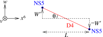
Figure -173: D4-branes tilted along $w$

The endpoints of D4-branes on the same NS5-brane interact with each other through a Coulomb interaction in the NS5 worldvolume. Because a D4-brane endpoint has codimension 2 in an NS5-brane worldvolume, the Coulomb potential goes logarithmically with the distance. In the present case, the D4-brane at $v$ and the one at $-v$ have a Coulomb potential energy $V_{C}$. In addition, there is potential energy coming from the tension of the D4-branes, which is $V_{T}=2T_{4}L$. Here, $T_{4}$ is the tension of a D4-brane and the factor $2$ is because we have two D4-branes. If the D4-branes were not tilted in the $w$ direction, i.e., if $\theta=0$, then the system would be supersymmetric and the two potentials would exactly cancel each other: $V_{C}+V_{T}^{\theta=0}=0$. However, if $\theta\neq 0$, the D4-branes are longer by $\Delta L=(L/\cos\theta)-L\approx L\theta^{2}/2$ than they are for $\theta=0$. As the result, $V_{T}$ gets increased by

$$\Delta V_{T}=V_{T}^{\theta}-V_{T}^{\theta=0}=2T_{4}\,\Delta L\approx{T_{4}\theta^{2}\over L}\approx{4T_{4}|\partial_{v}W|^{2}\over L}.$$ (7.6)

On the other hand, $V_{C}$ is not affected by $\theta$ because the Coulomb force depends only on the distance between D4-brane endpoints. Therefore, the total potential energy when $\theta\neq 0$ is given by

$$V_{sc}=V_{C}+V_{T}^{\theta}={4T_{4}|\partial_{v}W|^{2}\over L}.$$ (7.7)

The equation of motion derived from this potential energy is

$$0=\partial_{v}V_{sc}\propto{\partial_{v}^{2}W\over\partial_{v}W}-{\partial_{v}L\over L}.$$ (7.8)

One can interpret the first term in (7.8) as a force which pushes the D4-branes towards the values of $v$ for which $|\partial_{v}W|$ is smaller, and the second term as a force towards the values of $v$ for which $L$ is larger. As can be seen from (7.4), the latter force is logarithmic and tend to move the D4-branes toward large $|v|$. On the other hand, the former force is polynomial and can be tuned by choosing the polynomial $W(v)$. Therefore, it is natural to expect that, for any value of $v$, one can choose the superpotential $W(v)$ appropriately so that the equation of motion (7.8) is satisfied for that $v$. This is the geometric understanding of the metastable vacua found in [2].

As a quick check, let us compare the potential (7.7) obtained above with the potential energy in gauge theory. In the semiclassical regime where $|u_{2}|\gg|\Lambda|^{2}$, the moduli space metric for $u_{2}$ is known to be [7]:

$$g^{u_{2}\overline{u}_{2}} \approx{2\pi|u_{2}|\over\log\left|{u_{2}\over\Lambda^{2}}\right|}.$$ (7.9)

Therefore, the gauge theory potential is:

$$V_{gt} =g^{u_{2}\bar{u}_{2}}|\partial_{u_{2}}W|^{2}\approx{2\pi|u_{2}|\over\log\left|{u_{2}\over\Lambda^{2}}\right|}|\partial_{u_{2}}W|^{2}.$$ (7.10)

If we rewrite this in terms of $v=\sqrt{u_{2}}$,

$$V_{gt} ={\pi\over 2\log\left|{v\over\Lambda}\right|^{2}}|\partial_{v}W|^{2},$$ (7.11)

which agrees with the semiclassical potential (7.7) up to a numerical factor if we use (7.4). So, the potential (7.7) is indeed correct in the semiclassical regime.

One can also understand the parameter $\nu$ that appears in the exact M5 curve by a semiclassical reasoning, although strictly speaking $\nu$ is vanishing in the OOPP limit ($\nu={\cal O}(g^{2})$). If a D4-brane parallel to the $x^{6}$-axis is ending on an NS5-brane, then the lift, an M5-brane, has the following curve:

$$x^{6} =2R_{10}\log|v|=R_{10}(\log v+\log{\overline{v}}),\qquad x^{10}=2R_{10}\arg|v|=-iR_{10}(\log v-\log{\overline{v}}).$$ (7.12)

In the NS5 language, the $v$-dependence of $x^{6}$ represents the pull of the tension of the D4-brane along the $x^{6}$ direction, while the $v$-dependence of $x^{10}$ represents the flux inserted into the NS5 worldvolume by the D4-brane. Instead, if the D4-brane is not parallel to the $x^{6}$-axis but makes a small angle $\theta$ with it, then the tension will reduce by factor $\cos\theta$ and hence (7.12) is replaced by

$$x^{6} =R_{10}\cos\theta(\log v+\log{\overline{v}}),$$ (7.13)

whereas $x^{10}$ is unchanged because the amount of flux inserted by a D4 is independent of the angle between the D4 and the NS5. Therefore, $s=x^{6}+ix^{10}$ goes as

$$s =R_{10}[(\cos\theta+1)\log v+(\cos\theta-1)\log{\overline{v}}]\approx R_{10}\left[\left(2-{\theta^{2}\over 2}\right)\log v-{\theta^{2}\over 2}\log{\overline{v}}\right].$$ (7.14)

Comparing this with the expression of the exact curve (6.32), we obtain

$$\nu =-{\theta^{2}\over 2}=-{2|\partial_{v}W|^{2}\over L^{2}}.$$ (7.15)

We will see below that this is indeed satisfied in our M5-brane curve.

7.2 Semiclassical Limit of the M5 Curve

In the previous subsection, we showed that, in general, the semiclassical potential $V_{sc}$ (eq. (7.7)) and the gauge theory potential $V_{gt}$ are the same for $|v|\gg|\Lambda|$. Here we will check that the M5 curve obtained in section 6 satisfies the equations of motion derived from these potentials.

In the M5 curve (6.36), the quantities $\tau,\nu$ are determined in terms of the parameters $A_{6}$, $A_{4}$, $A_{2}$, $b_{2}$, or equivalently in terms of $(g,\beta,\gamma)$, $b_{2}$, by solving the last two equations in (6.32). In the semiclassical limit $\tau_{2}\gg 1$, $q=e^{i\pi\tau}$ is very small and we can use the $q$-expansions (D.1) to simplify those equations. After dropping all ${\cal O}(q)$ terms and subleading terms in $g$, we can write the resulting equations as follows:

$$\tau_{2} ={2(\beta v^{4}+\gamma v^{2}+1)\over\pi(5\beta v^{5}+3\gamma v^{2}+1)}={2\over\pi}{\partial_{v}W(v)\over v\,\partial_{v}^{2}W(v)}$$ (7.16a)

$$\nu =-{|gv|^{2}\over 2R_{10}^{2}}{(\overline{5\beta v^{5}+3\gamma v^{2}+1})^{2}(\beta v^{4}+\gamma v^{2}+1)\over\overline{\beta v^{4}+\gamma v^{2}+1}}=-2\left({|\partial_{v}W(v)|\over\pi g_{2}\tau_{2}}\right)^{2},$$ (7.16b)

where we have set $v=i\pi b_{2}$ and $\partial_{v}W=g(\beta v^{5}+\gamma v^{3}+v)$. Semiclassically, D4-branes are sitting at $v$ and $-v$.

Also, using the $q$-expansion (D.1) in (6.28), we obtain $q=\Lambda^{4}/64\pi^{4}b_{2}^{4}$. Therefore, we can express $\tau_{2}$ in terms of $v$ as follows:

$$\tau_{2}={1\over\pi}\log\left|{64\pi^{4}b_{2}^{4}\over\Lambda^{4}}\right|={1\over\pi}\log\left|{64v^{4}\over\Lambda^{4}}\right|\approx{2\over\pi}\log\left|{v\over\Lambda}\right|^{2}.$$ (7.17)

Therefore, (7.16a) can be written as

$${\partial_{v}^{2}W(v)\over\partial_{v}W(v)} ={2\over\pi v\tau_{2}}\approx{1/v\over\log\left|{v\over\Lambda}\right|^{2}}.$$ (7.18)

If we recall the expression for $L$, eq. (7.4), we immediately see that this is nothing but (7.8). So, indeed, the M-theory curve satisfies the semiclassical equation of motion derived from $V_{sc}$ or $V_{gt}$.

Similarly, one can show that the value of $\nu$ in the M5 curve given by (7.16b) agrees with the one given by the semiclassical expression (7.15). These agreements confirm that the reason for the existence of (meta)stable M5-brane configurations is the geometric mechanism discussed in the previous subsection.

As we show in Appendix E, we can also take the type IIA limit of the M5 curve, which is defined as the $R_{10}\to 0$ limit with the distance between the NS5’s kept fixed. In this limit, we end up with two NS5’s with D4’s stretching between them, and furthermore the log bending of NS5’s in the $x^{6}$ direction disappears. In order for the distance between the two D4’s to remain finite in the limit, we must take $\tau_{2}\to\infty$ as $\tau_{2}\sim 1/R_{10}$, as one can see in (E.7). Therefore, (7.16a) in this limit means that the D4’s sit at $v$ for which $\partial_{v}^{2}W(v)=w^{\prime}(v)=0$. This is understood as follows: In the IIA limit, there is no log bending of NS5’s along $x^{6}$ and the associated force, the second term in (7.8), is not there. So, the D4’s must sit at points where they can sit in equilibrium without any force (although unstable in this limit), which happens for $w^{\prime}(v)=0$. If one makes $R_{10}\neq 0$ and the quantum effects of bending are turned on, though, these points can be stabilized if the superpotential is properly tuned.

8 Concluding Remarks

In this paper, we demonstrated that the M5 lifts of NS5/D4 configurations which realize perturbed Seiberg-Witten theory accurately capture, in a suitable limit, the full scalar potential of the gauge theory and hence all nonsupersymmetric vacua that it describes. Within this regime, M5 configurations that approximately solve the equations of motion can be found and take the simple form of a holomorphic Seiberg-Witten geometry harmonically embedded along a transverse direction. These represent stringy realizations of the metastable vacua described by [2, 3]. Crucial to this story, however, was the fact that the scalar potential emerged only after the M5 worldvolume action was properly regularized. As such, the approximate solutions are not valid all the way out to $\infty$, but rather only within an appropriately chosen cutoff surface. We were able to make this completely explicit for the simple case of $SU(2)$ gauge group by finding exact solutions and demonstrating the existence of the appropriate “OOPP limit.”

Our $SU(2)$ example also allowed us to obtain a geometric understanding for the gauge theory potential, at least in the semiclassical limit, as well as the mechanism for stability. Stated in IIA language, the logarithmic bending of NS5’s by the D4’s which end on them creates pockets where the D4’s want to remain in order to minimize their length. The tendency to sit in these pockets, however, receives competition from the logarithmic repulsion of the D4’s stemming from their interaction through the NS5 worldvolumes. Nevertheless, one can suitably tune the asymptotic NS5 geometry in order to achieve stability. This is precisely the OOPP mechanism [2, 3] at work.

It should be noted that the story described here is quite similar to that considered in [1], where a different limit was studied. In that regime, the bending of the NS5’s is quite large and the lightest modes are fluctuations of the tubes into which the D4’s blow up in the M5 lift. The asymptotic $w(v)$ geometry is thus considered to be rigid with only $s(v)$ dynamical. Applying a $T$-duality along $x^{6}$ to this system, one obtains a deformed Calabi-Yau geometry determined by $w(v)$ with R and NS field strengths dual to $s(v)$. The limit of [1], then, corresponds on the IIB side to one in which the presence of nontrivial R and NS fluxes generates a potential for the moduli of a rigid Calabi-Yau. This potential can be computed in IIB [18] and is precisely equivalent to that which follows from the M5 worldvolume action along the lines of [1] and section 3. In light of this, it is natural to ask whether the scalar potential of perturbed Seiberg-Witten theory studied in this paper also has a type IIB counterpart. The most naive approach, namely $T$-dualizing along $x^{6}$, leads to an awkward regime in which nonnormalizable deformations of the geometry play a role in generating the potential for complex structure moduli rather than the fluxes. Applying $T$-duality along other directions, though, can lead to more natural constructions that are currently under investigation [66].

Appendix A Some Basic Results on Riemann Surfaces

In this appendix we summarize a few basic properties of Riemann surfaces, for more details see [67].

A compact Riemann surface $\Sigma_{g}$ is a one-dimensional compact complex manifold. Its topology is completely characterized by an integer, the genus $g$. The middle cohomology group has dimensionality $\dim H^{1}(\Sigma_{g})=2g$. The intersection form on $H_{1}(\Sigma_{g},\mathbb{Z})$ is antisymmetric and by Poincaré duality unimodular, which means that we can pick a basis of one-cycles $A_{i},B_{j}$ with intersection:

$$A_{i}\cap A_{j}=0,\quad B_{i}\cap B_{j}=0,\quad A_{i}\cap B_{j}=\delta_{ij}.$$ (A.1)

Such a basis is unique up to a symplectic transformation in $Sp(2g,\mathbb{Z})$,

A surface $\Sigma_{g}$ of genus $g$ has a complex structure moduli space ${\cal M}_{g}$ of dimensionality $\dim{\cal M}_{g}=3g-3,\,g\geq 2$.

A 1-form $\omega$ on a Riemann surface is called a holomorphic differential if in a local coordinate patch it has the form:

$$\omega=f(z)dz$$ (A.2)

with $f(z)$ holomorphic. We will also consider meromorphic differentials, for which we allow the function $f(z)$ to have poles at certain points on the surface. Now we present a standard basis for holomorphic and meromorphic differentials on a general Riemann surface:

Holomorphic differentials $\omega_{i}$:

Once we pick a symplectic basis of one-cycles, there is a canonical basis of holomorphic differentials $\omega_{i},i=1,..,g$, with the following periods:

$$\oint_{A_{i}}\omega_{j}=\delta_{ij},\qquad\oint_{B_{i}}\omega_{j}=\hat{\tau}_{ij}.$$ (A.3)

The (symmetric) matrix $\hat{\tau}_{ij}$ is the period matrix of the surface, and depends on the complex structure of $\Sigma_{g}$.

Meromorphic differentials of the second kind, $d\Omega_{n\geq 1}^{P}$:

These are characterized by a point $P$ on the surface where the differential has a pole of order $n+1$ with $n\geq 1$. The are normalized so that in local complex coordinates $z$ where $z(P)=0$ they have the Laurent expansion:

$$d\Omega^{P}_{n}\sim n{dz\over z^{n+1}}+\text{regular}.$$ (A.4)

Meromorphic differentials of the third kind, $d\Omega_{0}^{P,P^{\prime}}$:

characterized by two points $P,P^{\prime}$, where the differential has first order poles with opposite residues. Around $P$ we have:

$$d\Omega_{0}^{P,P^{\prime}}\sim{dz\over z}+\text{regular}$$ (A.5)

and similarly around $P^{\prime}$ with the opposite sign.

Notice that we can always shift a meromorphic differential by a holomorphic differential without changing the singular part of the Laurent expansions (A.4), (A.5). We can eliminate this ambiguity by demanding that the $A$ periods of the meromorphic differentials vanish:

$$\oint_{A_{i}}d\Omega_{n}^{P}=0.$$ (A.6)

In general, it is not possible to simultaneously set the $B$ periods to zero. Instead we have:

$$\oint_{B_{i}}d\Omega_{n}^{P}=K^{P}_{in},$$ (A.7)

where the matrix $K^{P}_{in}$ depends on the complex structure moduli of the Riemann surface and the position of the puncture $P$.

Harmonic functions on Riemann surfaces:

In two dimensions a function is harmonic if it satisfies $\partial\overline{\partial}f(z,\overline{z})=0$. Locally it is a sum of a holomorphic and an antiholomorphic function. On a compact surface, a harmonic function is necessarily constant. If we allow for poles at points $\{P_{a}\}$ we can also have nonconstant harmonic functions. They can be constructed using the meromorphic differentials. Consider the 1-form:

$$\omega=\sum_{a}\sum_{n\geq 1}T_{n}^{a}d\Omega^{P_{a}}_{n}+\sum_{a,b}T_{0}^{ab}d\Omega^{P_{a},P_{b}}_{0}+\sum_{i}h_{i}\omega_{i}+\text{c.c.}$$ (A.8)

Given $\omega$, locally we can always find a function $f$ such that $\omega=df$, and it is easy to see that $f$ is harmonic. To make sure the $f$ can be globally well defined on the Riemann surface, we must make sure that the compact periods of $\omega$ vanish:

$$\oint_{A_{i}}\omega=0,\quad\oint_{B_{i}}\omega=0$$ (A.9)

and that the total residue at each of the points $P_{a}$ vanishes.

Appendix B Parametric Representation of Genus 1 Seiberg-Witten Geometry

In this appendix, we describe the parametric representation of the genus 1 M5 curve of section 6.3 in more detail as a means of demonstrating basic techniques for manipulating the elliptic functions $F_{i}^{(n)}$ . In particular, we focus on the M5 lift of an NS5/D4 configuration of the type depicted in figure -179(a) with two parallel NS5’s extended along $v$ and two D4-branes suspended in between. The M5 lift has genus 1 and can be described by two embedding functions $s(z)$ and $v(z)$ defined on the fundamental parallelogram of figure -175(b). As discussed in section 6.3, $s(z)$ and $v(z)$ take the form

$$\begin{split}v(z)&=b_{2}\left(F_{1}^{(1)}-F_{2}^{(1)}+i\pi\right),\\ s(z)&=2\left(F_{1}-F_{2}+i\pi z\right).\end{split}$$ (B.1)

Moreover, one of the $\hat{B}$-period constraints for $ds$ fixes the distance between the marked points in terms of $\tau$

$$a\equiv a_{2}-a_{1}=\frac{\tau}{2}.$$ (B.2)

The other $\hat{B}$-period constraint determines how the dynamical scale $\Lambda$ is related to curve parameters. Rather than studying the $\hat{B}$-period constraint directly, though, let us instead try to determine the explicit relationship between $v(z)$ and $s(z)$ in (B.1) and read it off from the Seiberg-Witten geometry (recall that $t\equiv\Lambda^{N}e^{-s}$)

$$t^{2}-2P_{N}(v)t+\Lambda^{2N}=0.$$ (B.3)

It is easiest to work with elliptic functions so, to start, we study the derivative of $s$. This leads us to observe that

$$ds=2\left(F_{1}^{(1)}-F_{2}^{(1)}+i\pi\right)dz=\frac{2v\,dz}{b_{2}}.$$ (B.4)

From this, it is clear that we can easily determine $s(v)$ by integration once we are able to write $\frac{dv}{dz}$ as a function of $v$. As such, we turn to

$$G(z)\equiv\frac{dv}{dz}=b_{2}\left(F_{1}^{(2)}-F_{2}^{(2)}\right)$$ (B.5)

and seek an algebraic relationship between the elliptic functions $G(z)$ and $v(z)$. Because $G(z)$ has second order poles while $v(z)$ has first order ones, our first guess might be that $G(z)$ is given by a quadratic polynomial in $v(z)$. This is impossible, though, because the second order poles of $G(z)$ have opposite signs while those of $v(z)^{2}$ have the same sign. Because of this, we instead consider the possibility that $G(z)^{2}$ is equivalent to a quartic polynomial in $v(z)$ 

$$G(z)^{2}-b_{2}^{2}\left(v^{4}+C_{1}v^{2}+C_{2}\right)=0.$$ (B.6)

Because the LHS of this equation is an elliptic function, it is completely specified, up to a constant shift, by its pole structure. As such, we need only verify that it vanishes at the marked points $a_{1}$ and $a_{2}$. The coefficients of the poles at $a_{1}$ and $a_{2}$ are equivalent up to possible minus signs, though, so we only need to study $G(z)^{2}$ and $v(z)^{m}$ in the vicinity of one marked point, say $a_{1}$. Expanding $G(z)^{2}$, we find

$$\begin{split}G(z)^{2}&=b_{2}^{2}\left(F_{1}^{(2)}-F_{2}^{(2)}\right)^{2}\\ &\sim\frac{b_{2}^{2}}{(z-a_{1})^{4}}-\frac{2b_{2}^{2}\wp(\tau/2)}{(z-a_{1})^{2}}+b_{2}^{2}\left(\frac{3g_{2}}{5}-5\wp(\tau/2)^{2}\right)+{\cal{O}}(z-a_{1}).\end{split}$$ (B.7)

On the other hand,

$$\frac{1}{b_{2}^{2}}\left(v^{4}+C_{1}v^{2}+C_{2}\right)\sim\frac{b_{2}^{2}}{(z-a_{1})^{4}}+\frac{C_{1}+4b_{2}^{2}\wp(\tau/2)}{(z-a_{1})^{2}}\\ +\left(\frac{C_{2}}{b_{2}}^{2}-\frac{2b_{2}^{2}g_{2}}{5}+2C_{1}\wp(\tau/2)+10b_{2}^{2}\wp(\tau/2)^{2}\right)+{\cal{O}}(z-a_{1}).$$ (B.8)

From this, we see that

$$G(z)^{2}=\frac{1}{b_{2}^{2}}\left[\left(v(z)^{2}-3b_{2}^{2}\wp(\tau/2)\right)^{2}+b_{2}^{4}\left(g_{2}-12\wp(\tau/2)^{2}\right)\right].$$ (B.9)

Returning to (B.4), this implies that

$$ds=-\frac{2v\,dv}{\sqrt{\left(v^{2}-3b_{2}^{2}\wp(\tau/2)\right)^{2}+b_{2}^{4}\left(g_{2}-12\wp(\tau/2)^{2}\right)}},$$ (B.10)

which can be integrated to yield

$$s(v)=-\ln\left(v^{2}-u-\sqrt{(v^{2}-u)^{2}-\Lambda^{4}}\right)+\text{constant},$$ (B.11)

where

$$u=3b_{2}^{2}\wp(\tau/2)\qquad\Lambda^{4}=b_{2}^{4}\left(12\wp(\tau/2)^{2}-g_{2}\right).$$ (B.12)

Our choice of notation $u$ and $\Lambda$ is already quite suggestive. Indeed, it is easy to demonstrate now that, dropping the constant in (B.11), $t=\Lambda^{2}e^{-s}$ satisfies

$$t^{2}-2P_{2}(v)t+\Lambda^{4}=0$$ (B.13)

for

$$P_{2}(v)=v^{2}-u.$$ (B.14)

This justifies our identification of $\Lambda$ in (B.12). In particular, we see that the constant $b_{2}$ is now fixed in terms of $\tau$ and $\Lambda$. The only free parameter left in our solution, then, is $\tau$. While this provides a perfectly fine parametrization of the moduli space, a more conventional one is given by $u_{2}$ (4.3). The relation between $u_{2}$ and $\tau$ can be read off directly from (B.12) as $u_{2}$ should be identified the parameter $u$ there. We can also use (4.7), however, to compute $u_{2}(\tau)$ directly from our parametric description (B.1)

$$\begin{split}u_{2}&=\frac{1}{4\pi i}\oint_{a_{1}}v^{2}\,ds\\ &=\frac{1}{4\pi i}\oint_{a_{1}}\,2b_{2}^{2}\left(F_{1}^{(1)}-F_{2}^{(1)}+i\pi\right)^{3}\,dz.\end{split}$$ (B.15)

This can be easily evaluated by expanding $F_{1}^{(1)}$ and $F_{2}^{(1)}$ near $a_{1}$ and results in

$$u_{2}=3b_{2}^{2}\wp(\tau/2).$$ (B.16)

Consequently, $u_{2}$ is nothing other than the parameter $u$ in (B.12).

Appendix C Symmetry Argument for the Ansatz (6.32)

In this Appendix, we motivate the ansatz (6.32) for the M5 curve describing the OOPP vacua from a symmetry argument.

First, let us examine the symmetry of the M5 curve in the supersymmetric case. As explained in section 2, an M5 curve corresponding to supersymmetric vacuum of $SU(2)$ theory has the following form:

$$t^{2}-2P_{N}(v)t+\Lambda^{2N}=0,$$ (C.1)

$$w(v)=\sqrt{W_{n}^{\prime}(v)^{2}-f_{n-1}(v)},$$ (C.2)

where $t=\Lambda^{N}e^{-s}$, and satisfies the constraint (2.14) or (2.15). Because in the $SU(2)$ case $\mathop{\mathrm{Tr}}\nolimits\Phi^{k}=0$ for odd $k$, $P_{2}(v)=v^{2}-u_{2}$ and $W_{n}^{\prime}(v)$ has only odd powers in $v$. By examining (2.14), (2.15), one can see that this implies that $f_{n-1}(v)$ has only even powers in $v$. Accordingly, under $v\to-v$,

$$P_{2}(v) \to P_{2}(v),\qquad W^{\prime}_{n}(v)\to-W^{\prime}_{n}(v),\qquad f_{n-1}(v)\to f_{n-1}(v).$$ (C.3)

From (C.1), one obtains

$$s(v)=\ln\left({P_{2}(v)+\sqrt{P_{2}(v)^{2}-\Lambda^{4}}\over\Lambda^{2}}\right).$$ (C.4)

The relations (C.2) and (C.4) define the $w,s$ coordinates as functions on the two-sheeted cover of the complex $v$ plane.

This supersymmetric curve has the following symmetries:

$$\begin{split}\text{symmetry I)}&\quad v\to-v\text{~{}(same sheet)},\quad w\to-w,\quad s\to s;\\ \text{symmetry II)}&\quad v\to v\text{~{}(different sheet)},\quad w\to-w,\quad s\to-s.\end{split}$$ (C.5)

For example, if we flip $v\to-v$ remaining on the same sheet, then from (C.2)–(C.4) it is easy to see that $w=\sqrt{W_{n}^{\prime}{}^{2}+f_{n-1}}=W_{n}^{\prime}+{f_{n-1}\over 2W_{n}}+\cdots\to-W_{n}^{\prime}-{f_{n-1}\over 2W_{n}}-\cdots=-w$ and $s\to s$ (symmetry I). On the other hand, if move $v$ between the first and second sheets, the square roots in (C.2) and (C.4) flip their signs and we have $w\to-w$, $s\to-s$ (symmetry II).

Because we will write M5 curves in parametric representation on the $z$ plane, we need to implement these symmetries (C.5) on the $z$ plane. In the supersymmetric case, the relation between $v$ and $z$ is given by (6.22). Using the properties of $F^{(1)}_{i}(z)$ in (6.17), one can see that, if $a=a_{2}-a_{1}=\tau/2$,

$$\begin{array}[]{r@{\,}lcr@{\,}l}\text{transformation I) }\qquad v&\to-v\text{~{}(same sheet)}&\Longleftrightarrow&z&\to 2a_{1}-z\cong 2a_{2}-z,\\[2.15277pt] \text{transformation II)}\qquad v&\to v\text{~{}(different sheet)}&\Longleftrightarrow&z&\to a_{1}+a_{2}-z.\end{array}$$ (C.8)

Let us require that the exact M5 curve corresponding to the OOPP vacuum have the same symmetries as above. Namely, under the transformations of $z$ in (C.8), we require that $s,v,w$ transform according to (C.5). The 1-forms $ds,dv,dw$ have the same transformation property as $s,v,w$. The basis of 1-forms $\omega$, $d\Omega_{0}^{a_{1},a_{2}}$, $d\Omega_{n\geq 1}^{a_{i}}$, $i=1,2$ introduced in section 6.2 have the following transformation property under the transformations (C.8):

$$\begin{split}\text{I)}\quad&\omega\to-\omega,\quad d\Omega_{0}^{a_{1},a_{2}}\to+d\Omega_{0}^{a_{1},a_{2}},\quad d\Omega_{n}^{a_{1}}\to(-1)^{n}d\Omega_{n}^{a_{1}},\quad d\Omega_{n}^{a_{2}}\to(-1)^{n}d\Omega_{n}^{a_{2}},\\ \text{II)}\quad&\omega\to-\omega,\quad d\Omega_{0}^{a_{1},a_{2}}\to-d\Omega_{0}^{a_{1},a_{2}},\quad d\Omega_{n}^{a_{1}}\to(-1)^{n}d\Omega_{n}^{a_{2}},\quad d\Omega_{n}^{a_{2}}\to(-1)^{n}d\Omega_{n}^{a_{1}}.\end{split}$$ (C.9)

Therefore, in order to obey (C.5), the 1-forms $ds,dv,dw$ must have the following schematic form:

$$\begin{split}dw&\sim\sum_{n=1,3,5,\dots}(d\Omega_{n}^{a_{1}}+d\Omega_{n}^{a_{2}})+\omega+{\rm c.c.},\\ dv&\sim\sum_{n=1,3,5,\dots}(d\Omega_{n}^{a_{1}}-d\Omega_{n}^{a_{2}})+{\rm c.c.},\\ ds&\sim d\Omega_{0}^{a_{1},a_{2}}+{\rm c.c.},\end{split}$$ (C.10)

where coefficients are omitted. In other words,

$$\begin{split}dw&\sim\sum_{n=2,4,6,\dots}(F_{1}^{(n)}+F_{2}^{(n)})dz+dz+{\rm c.c.},\\ dv&\sim\sum_{n=2,4,6,\dots}(F_{1}^{(n)}-F_{2}^{(n)})dz+{\rm c.c.},\\ ds&\sim(F_{1}^{(1)}-F_{2}^{(1)}+i\pi)dz+{\rm c.c.}\end{split}$$ (C.11)

So far we have not taken into account any period constraints but, in $dw$, $(F_{1}^{(2)}+F_{2}^{(2)})dz$ must come with $dz-d{\overline{z}}$ for the period along $\hat{B}_{2}-\hat{B}_{1}$ to vanish. Therefore, $dw$ must come with

$$(F_{1}^{(2)}+F_{2}^{(2)})dz+{4\pi i\over\tau-{\overline{\tau}}}(dz-d{\overline{z}}).$$ (C.12)

In the small superpotential case studied in section 4, $v(z)$ was given by (6.22) and $dv(z)$ had order two poles at $z=a_{1,2}$. To consider the OOPP vacuum, we would like to take a degree six superpotential, which leads to the boundary condition (5.10). This motivates us to study $dw(z)$ that has up to order six poles at $z=a_{1,2}$ and therefore contains $F^{(n)}_{i}$ with $n\leq 6$. However, as was discussed below (6.31), the pole structure of $v(z)$ given by (6.22) is not enough; in order to satisfy the Virasoro constraint we need to include higher order poles in $dv(z)$ than was considered in (6.22). In the present case, order four poles are sufficient. After all, we are led to the following ansatz:

$$\begin{split}dw&\sim(F_{1}^{(6)}+F_{2}^{(6)})dz+(F_{1}^{(4)}+F_{2}^{(4)})dz+(F_{1}^{(2)}+F_{2}^{(2)})dz+{4\pi i\over\tau-{\overline{\tau}}}(dz-d{\overline{z}}),\\ dv&\sim(F_{1}^{(4)}-F_{2}^{(4)})dz+(F_{1}^{(2)}-F_{2}^{(2)})dz+{\rm c.c.},\\ ds&\sim(F_{1}^{(1)}-F_{2}^{(1)}+i\pi)dz+{\rm c.c.},\end{split}$$ (C.13)

which upon integration becomes the ansatz (6.32) that we used.

Appendix D $q$-expansions

When $\tau_{2}\gg 1$, $q=e^{i\pi\tau}=e^{i\pi\tau_{1}-\pi\tau_{2}}$ is small and the following $q$-expansions [1, 68] are useful:

$$\begin{split}F(z)&=\ln(e^{2\pi iz}-1)+\ln\left[1+\sum_{k=1}^{\infty}(2k+1)(-1)^{k}q^{k(k+1)}\right]+4\sum_{k=1}^{\infty}{q^{2k}\sin^{2}(k\pi z)\over k(1-q^{2k})},\\ \wp\left({\tau\over 2}\right)&=-\frac{\pi^{2}}{3}-8\pi^{2}\sum_{k=1}^{\infty}\frac{kq^{k}}{1+q^{k}},\qquad\qquad\eta_{1}=\frac{\pi^{2}}{6}-4\pi^{2}\sum_{k=1}^{\infty}\frac{kq^{2k}}{1-q^{2k}},\\ g_{2}&={4\pi^{4}\over 3}\left(1+240\sum_{k=1}^{\infty}\frac{k^{3}q^{2k}}{1-q^{2k}}\right),\qquad\qquad g_{3}={8\pi^{6}\over 27}\left(1-504\sum_{k=1}^{\infty}\frac{k^{5}q^{2k}}{1-q^{2k}}\right).\end{split}$$ (D.1)

Note also that $\eta_{1},\eta_{3}$ are related by $\eta_{1}\tau-\eta_{3}=i\pi$.

Appendix E Type IIA Limit of the M5 Curve

In this Appendix, we consider the type IIA limit of the M5 curve in the OOPP limit obtained in section 6.6. The IIA limit is defined to be the $R_{10}\to 0$ limit with the distance between NS5’s and that between D4’s kept finite. We will see that, in the limit, we end up with curved NS5-branes along $w=\pm W^{\prime}(v)$ with D4-branes stretched in between, and that there is no logarithmic bending of NS5-branes along the $x^{6}$ direction. As a result, we will see that D4-branes sit at the critical point of $w(v)$, namely at $v$ for which $W^{\prime\prime}(v)=0$.

The M5 curve in the OOPP limit obtained in section 6.6 can be written as:

$$\begin{split}s&=2\left[F_{1}-F_{2}+i\pi(z-A-a)\right],\\ v&=b_{2}(F_{1}^{(1)}-F_{2}^{(1)}+i\pi),\\ w&=A_{6}(F_{1}^{(5)}+F_{2}^{(5)})+A_{4}(F_{1}^{(3)}+F_{2}^{(3)})+A_{2}\left[(F_{1}^{(1)}+F_{2}^{(1)})+{4\pi i\over\tau_{2}}\mathop{\mathrm{Im}}\nolimits(z-A-a)\right].\end{split}$$ (E.1)

where the parameters $A_{2,4,6}$ are related to the coefficients $g,\beta,\gamma$ in the superpotential (5.9) and (5.10) via (6.40). Given these parameters, the modulus $\tau$ is determined by solving (6.43). Recall also that $a\equiv a_{2}-a_{1}={\tau/2}$ and $A\equiv(a_{1}+a_{2})/2$. The constants in (E.1) have been chosen for later convenience.

In the type IIA limit where the distance between the tubes is much larger than the size of the tubes, $\tau_{2}\gg 1$. In this limit, $q=e^{i\pi\tau}=e^{i\pi\tau_{1}-\pi\tau_{2}}$ is very small and, using (D.1), we can approximate $F(z)$ as

$$F(z) \approx\ln(e^{2\pi iz}-1).$$ (E.2)

Therefore, for example, we can approximate $s,v$ in (E.1) as

$$\begin{split}s&\approx 2\left[\log\left({e^{2\pi i(z-a_{1})}-1\over e^{2\pi i(z-a_{2})}-1}\right)+i\pi(z-A-a)\right],\\ v&\approx 2\pi ib_{2}\left[{1\over 1-e^{-2\pi i(z-a_{1})}}-{1\over 1-e^{-2\pi i(z-a_{2})}}+{\frac{1}{2}}\right].\end{split}$$ (E.3)

We can similarly obtain an approximate form for $w$, but we do not display it here explicitly because it is too lengthy. On the other hand, applying (D.1) to (6.29), we see that, in the large $\tau_{2}$ limit, $u_{2}\approx-\pi^{2}b_{2}^{2}.$ Classically, the two tubes are sitting at the solution to $P_{2}(v)=0$, namely at $v=\pm\sqrt{u_{2}}\approx\pm i\pi b_{2}$. Therefore, if we want to keep the distance between the two tubes to be finite, we must keep $b_{2}$ finite.

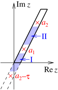
Figure -172: The $z$-torus for large $\tau_{2}$. Region I ($\mathop{\mathrm{Im}}\nolimits(z-a_{1})\ll 0$, $\mathop{\mathrm{Im}}\nolimits(z-a_{2})\ll 0$) and region II ($\mathop{\mathrm{Im}}\nolimits(z-a_{1})\gg 0$, $\mathop{\mathrm{Im}}\nolimits(z-a_{2})\ll 0$) are depicted as shaded regions.

In the type IIA limit, we take $R_{10}\to 0$ by definition. What is the relation between $\tau_{2}$ and $R_{10}$ in this limit? For this, let us look at the behavior of $s$ and $v$ near $z=a_{1,2}$, where they blow up. By examining (E.3), it is easy to see that, near $z=a_{1,2}$,

$$s \sim\pm 2\left[\log\left({2\pi ib_{2}\over v}\right)+{\frac{1}{2}}i\pi a\right].$$ (E.4)

So, the distance between two NS5’s at $v=v_{0}$ is given by

$$L \equiv R_{10}\mathop{\mathrm{Re}}\nolimits\bigl{[}s(z=a_{1})-s(z=a_{2})\bigr{]}=4R_{10}\left(\log\left|{2\pi b_{2}\over v_{0}}\right|-{\pi\tau_{2}\over 4}\right).$$ (E.5)

In other words,

$$|b_{2}|={|v_{0}|\over 2\pi}e^{{1\over 4}\left(\pi\tau_{2}-{L\over R_{10}M}\right)}.$$ (E.6)

In the IIA limit, we send $R_{10}\to 0$ keeping $L$ and $b_{2}$ finite. Therefore, we must send $\tau_{2}\to\infty$ as $R_{10}\to 0$, as

$$\tau_{2}\sim{L\over\pi R_{10}}.$$ (E.7)

If $\tau_{2}$ is very large, the $z$-torus becomes very long vertically (along the $\mathop{\mathrm{Im}}\nolimits z$ axis) as in Figure -172. We expect that the long, narrow regions “between” marked points correspond to tubes that descend to D4-branes in the IIA limit. More specifically, let us call the region where $\mathop{\mathrm{Im}}\nolimits(z-a_{1})\ll 0$, $\mathop{\mathrm{Im}}\nolimits(z-a_{2})\ll 0$ “region I” and the region where $\mathop{\mathrm{Im}}\nolimits(z-a_{1})\gg 0$, $\mathop{\mathrm{Im}}\nolimits(z-a_{2})\ll 0$ “region II” (see Figure -172). Let us see that regions I and II correspond to two D4’s in the IIA limit.

In region I, using (E.3) and (E.2), one can readily derive

$$\begin{split}s&\approx 2\pi i(z+a-A),\\ v&\approx i\pi b_{2},\qquad\qquad\qquad\qquad\text{(region I)}\\ w&\approx{4\pi iA_{2}\over\tau_{2}}(z+a-A).\end{split}$$ (E.8)

So, if we move from $z=a_{2}-\tau$ (in the fundamental parallelogram below our fundamental parallelogram) to $z=a_{1}$, then $s,v,w$ change linearly as

$$\begin{array}[]{r@{\,}lcr@{\,}l}s&=-{\frac{1}{2}}\pi i\tau&\to&s&={\frac{1}{2}}\pi i\tau,\\[2.15277pt] v&=i\pi b_{2}&\to&v&=i\pi b_{2},\\[2.15277pt] w&=-i\pi A_{2}&\to&w&=i\pi A_{2}.\end{array}$$ (E.12)

The change in $x^{6}$ is

$$\Delta x^{6}=R_{10}\mathop{\mathrm{Re}}\nolimits(\Delta s)=-\pi R_{10}\tau_{2}=-L,$$ (E.13)

where in the last equality we used (E.7). Therefore, region I indeed corresponds to a D4-brane at $v=i\pi b_{2}$ with length $L$ along $x^{6}$. Note also that this D4 is tilted along $w$ by $\Delta w=2\pi iA_{2}$. Similarly, one can show that region II corresponds to a D4-brane at $v=-i\pi b_{2}$ with length $L$ along $x^{6}$, tilted along $w$ by $\Delta w=-2\pi iA_{2}$.

Now let us turn to the regions near $z=a_{1,2}$, which must correspond to NS5’s curved along (6.39). Near $z=a_{1}$,

$$s \approx 2\left[\log(2\pi i(z-a_{1}))+{i\pi\tau\over 4}\right],\qquad v\approx{b_{2}\over 2\pi i(z-a_{1})}\qquad\qquad(z\approx a_{1}).$$ (E.14)

If we eliminate $z$,

$$v =2\pi ib_{2}e^{-{s\over 2}+{i\pi\tau\over 2}}.$$ (E.15)

Note that

$$\left|e^{-{s\over 2}+{i\pi\tau\over 2}}\right|=e^{-{x^{6}\over 2R_{10}}-{\pi\tau_{2}\over 4}}=e^{-{1\over 2R_{10}}(x^{6}+{L\over 2})}.$$ (E.16)

This goes to zero in the $R_{10}\to 0$ limit unless $x^{6}$ is very close to $-L/2$, where the left NS5 sits. If $x^{6}$ is very close to $-{L/2}$, within ${\cal O}(R_{10})$, then we can tune $x^{6}+{L/2}$ to allow $v$ to take any value in ${\mathbb{C}}$. Namely, we see that the region near $z=a_{1}$ indeed corresponds to the left NS5 sitting at $x^{6}=-{L/2}$ and extending in the $v$ direction. How about the $w$ direction? $w$ goes, near $z=a_{1}$, as

$$w \approx{24A_{6}\over(z-a_{1})^{5}}+{2A_{4}\over(z-a_{1})^{3}}+{A_{2}\over z-a_{1}}\qquad\qquad(z\approx a_{1}).$$ (E.17)

To see the relation between $v$ and $w$, we need the expression for $v$ up to lower powers in $(z-a_{1})$ than was needed in (E.14). Near $z=a_{1},$

$$v \approx 2\pi ib_{2}\left[{1\over 1-e^{-2\pi i(z-a_{1})}}-{\frac{1}{2}}\right]\qquad\qquad(z\approx a_{1}).$$ (E.18)

If we eliminate $(z-a_{1})$ from (E.17) and (E.18), we obtain

$$w ={24A_{6}\over b^{5}}v^{5}+{2(A_{4}+20\pi^{2}A_{6})\over b_{2}^{3}}v^{3}+{A_{2}+2\pi^{2}A_{4}+16\pi^{4}A_{6}\over b_{2}}v+{\cal O}\left({1\over v}\right).$$ (E.19)

One can readily see that this is the expected behavior (6.39), if one uses (6.40) and that $\wp(\tau/2)\approx-\pi^{2}/3$, $g_{2}\approx 4\pi^{4}/3$ for large $\tau_{2}$.

Similarly, one can show that the region near $z=a_{2}$ corresponds to an NS5 at $x^{6}=L/2$ along $w=-W^{\prime}(v)$.

So far we have been treating the parameters $A_{2,4,6},b_{2},\tau_{2}$ as if they were all arbitrary, but they are actually subject to the constraint (6.43). For large $\tau_{2}$, this equation reduces to (7.16a):

$$\tau_{2} ={2\over\pi}{W^{\prime}(v)\over vW^{\prime\prime}(v)}.$$ (E.20)

where $v=\pm i\pi b_{2}$. An important difference from the semiclassical limit considered in section 7 is that we send $\tau_{2}\to\infty$ as (E.7) as we take $R_{10}\to 0$. This means that

$${vW^{\prime\prime}(v)\over W^{\prime}(v)}={2\over\pi\tau_{2}}={2R_{10}\over L}\to 0.$$ (E.21)

Therefore, in the IIA limit, the D4’s must sit at a critical point of $w(v)=W^{\prime}(v)$, i.e., it must be that $w^{\prime}(v)=0$. This is because in the IIA limit the log bending of NS5’s along $x^{6}$ disappears and hence there is no force to cancel the $w$-tilting force. So, the D4’s must sit at points where they can sit in equilibrium without any force (although unstable in this limit), which happens for $w^{\prime}(v)=0$.

References

- [1] J. Marsano, K. Papadodimas and M. Shigemori, “Nonsupersymmetric brane / antibrane configurations in type IIA and M theory,” Nucl. Phys. B 789, 294 (2008) [arXiv:0705.0983 [hep-th]].
- [2] H. Ooguri, Y. Ookouchi and C. S. Park, “Metastable Vacua in Perturbed Seiberg-Witten Theories,” arXiv:0704.3613 [hep-th].
- [3] G. Pastras, “Non supersymmetric metastable vacua in N = 2 SYM softly broken to N = 1,” arXiv:0705.0505 [hep-th].
- [4] E. Witten, “Solutions of four-dimensional field theories via M-theory,” Nucl. Phys. B 500, 3 (1997) [arXiv:hep-th/9703166].
- [5] E. Witten, “Branes and the dynamics of QCD,” Nucl. Phys. B 507, 658 (1997) [arXiv:hep-th/9706109].
- [6] A. Giveon and D. Kutasov, “Brane dynamics and gauge theory,” Rev. Mod. Phys. 71, 983 (1999) [arXiv:hep-th/9802067].
- [7] N. Seiberg and E. Witten, “Electric - magnetic duality, monopole condensation, and confinement in N=2 supersymmetric Yang-Mills theory,” Nucl. Phys. B 426, 19 (1994) [Erratum-ibid. B 430, 485 (1994)] [arXiv:hep-th/9407087].
- [8] N. Seiberg and E. Witten, “Monopoles, duality and chiral symmetry breaking in N=2 supersymmetric QCD,” Nucl. Phys. B 431, 484 (1994) [arXiv:hep-th/9408099].
- [9] K. Intriligator, N. Seiberg and D. Shih, “Dynamical SUSY breaking in meta-stable vacua,” JHEP 0604, 021 (2006) [arXiv:hep-th/0602239].
- [10] S. Franco and A. M. Uranga, “Dynamical SUSY breaking at meta-stable minima from D-branes at obstructed geometries,” JHEP 0606, 031 (2006) [arXiv:hep-th/0604136].
- [11] I. Garcia-Etxebarria, F. Saad and A. M. Uranga, “Local models of gauge mediated supersymmetry breaking in string theory,” JHEP 0608, 069 (2006) [arXiv:hep-th/0605166].
- [12] H. Ooguri and Y. Ookouchi, “Landscape of supersymmetry breaking vacua in geometrically realized gauge theories,” Nucl. Phys. B 755, 239 (2006) [arXiv:hep-th/0606061].
- [13] H. Ooguri and Y. Ookouchi, “Meta-stable supersymmetry breaking vacua on intersecting branes,” Phys. Lett. B 641, 323 (2006) [arXiv:hep-th/0607183].
- [14] S. Franco, I. Garcia-Etxebarria and A. M. Uranga, “Non-supersymmetric meta-stable vacua from brane configurations,” JHEP 0701, 085 (2007) [arXiv:hep-th/0607218].
- [15] I. Bena, E. Gorbatov, S. Hellerman, N. Seiberg and D. Shih, “A note on (meta)stable brane configurations in MQCD,” JHEP 0611, 088 (2006) [arXiv:hep-th/0608157].
- [16] C. Ahn, “Brane configurations for nonsupersymmetric meta-stable vacua in SQCD with adjoint matter,” Class. Quant. Grav. 24, 1359 (2007) [arXiv:hep-th/0608160], “M-theory lift of meta-stable brane configuration in symplectic and orthogonal gauge groups,” Phys. Lett. B 647, 493 (2007) [arXiv:hep-th/0610025], “Meta-stable brane configuration with orientifold 6 plane,” JHEP 0705, 053 (2007) [arXiv:hep-th/0701145], “More on Meta-Stable Brane Configuration,” Class. Quant. Grav. 24, 3603 (2007) [arXiv:hep-th/0702038], “Meta-Stable Brane Configuration and Gauged Flavor Symmetry,” Mod. Phys. Lett. A 22, 2329 (2007) [arXiv:hep-th/0703015], “Meta-Stable Brane Configurations by Adding an Orientifold-Plane to Giveon-Kutasov,” JHEP 0708, 021 (2007) [arXiv:0706.0042 [hep-th]], “More Meta-Stable Brane Configurations without D6-Branes,” Nucl. Phys. B 790, 281 (2008) [arXiv:0707.0092 [hep-th]].
- [17] R. Argurio, M. Bertolini, S. Franco and S. Kachru, “Gauge/gravity duality and meta-stable dynamical supersymmetry breaking,” JHEP 0701, 083 (2007) [arXiv:hep-th/0610212];
- [18] M. Aganagic, C. Beem, J. Seo and C. Vafa, “Geometrically induced metastability and holography,” Nucl. Phys. B 789, 382 (2008) [arXiv:hep-th/0610249].
- [19] R. Tatar and B. Wetenhall, “Metastable vacua, geometrical engineering and MQCD transitions,” JHEP 0702, 020 (2007) [arXiv:hep-th/0611303].
- [20] R. Kitano, H. Ooguri and Y. Ookouchi, “Direct mediation of meta-stable supersymmetry breaking,” Phys. Rev. D 75, 045022 (2007) [arXiv:hep-ph/0612139].
- [21] J. J. Heckman, J. Seo and C. Vafa, “Phase Structure of a Brane/Anti-Brane System at Large N,” JHEP 0707, 073 (2007) [arXiv:hep-th/0702077];
- [22] A. Giveon and D. Kutasov, “Gauge symmetry and supersymmetry breaking from intersecting branes,” Nucl. Phys. B 778, 129 (2007) [arXiv:hep-th/0703135].
- [23] R. Argurio, M. Bertolini, S. Franco and S. Kachru, “Metastable vacua and D-branes at the conifold,” JHEP 0706, 017 (2007) [arXiv:hep-th/0703236].
- [24] S. Murthy, “On supersymmetry breaking in string theory from gauge theory in a throat,” JHEP 0708, 013 (2007) [arXiv:hep-th/0703237].
- [25] I. Garcia-Etxebarria, F. Saad and A. M. Uranga, “Supersymmetry breaking metastable vacua in runaway quiver gauge theories,” JHEP 0705, 047 (2007) [arXiv:0704.0166 [hep-th]].
- [26] T. Kawano, H. Ooguri and Y. Ookouchi, “Gauge Mediation in String Theory,” Phys. Lett. B 652, 40 (2007) [arXiv:0704.1085 [hep-th]].
- [27] M. R. Douglas, J. Shelton and G. Torroba, “Warping and supersymmetry breaking,” arXiv:0704.4001 [hep-th].
- [28] D. Malyshev, “Del Pezzo singularities and SUSY breaking,” arXiv:0705.3281 [hep-th].
- [29] R. Tatar and B. Wetenhall, “Metastable Vacua and Complex Deformations,” Phys. Rev. D 76, 126011 (2007) [arXiv:0707.2712 [hep-th]].
- [30] O. Aharony and S. Kachru, “Stringy Instantons and Cascading Quivers,” JHEP 0709, 060 (2007) [arXiv:0707.3126 [hep-th]].
- [31] J. J. Heckman and C. Vafa, “Geometrically Induced Phase Transitions at Large N,” arXiv:0707.4011 [hep-th].
- [32] O. Aharony, S. Kachru and E. Silverstein, “Simple Stringy Dynamical SUSY Breaking,” Phys. Rev. D 76, 126009 (2007) [arXiv:0708.0493 [hep-th]].
- [33] M. Aganagic, C. Beem and B. Freivogel, “Geometric Metastability, Quivers and Holography,” arXiv:0708.0596 [hep-th].
- [34] J. Kumar, “Dynamical SUSY Breaking in Intersecting Brane Models,” arXiv:0708.4116 [hep-th].
- [35] L. Mazzucato, Y. Oz and S. Yankielowicz, “Supersymmetry Breaking Vacua from M Theory Fivebranes,” arXiv:0709.2491 [hep-th].
- [36] M. Aganagic, C. Beem and S. Kachru, “Geometric Transitions and Dynamical SUSY Breaking,” arXiv:0709.4277 [hep-th];
- [37] A. Giveon and D. Kutasov, “Stable and Metastable Vacua in SQCD,” arXiv:0710.0894 [hep-th].
- [38] A. Giveon and D. Kutasov, “Stable and Metastable Vacua in Brane Constructions of SQCD,” arXiv:0710.1833 [hep-th].
- [39] M. Buican, D. Malyshev and H. Verlinde, “On the Geometry of Metastable Supersymmetry Breaking,” arXiv:0710.5519 [hep-th].
- [40] R. Tatar and B. Wetenhall, “SQCD Vacua and Geometrical Engineering,” arXiv:0711.2534 [hep-th].
- [41] H. Verlinde and M. Wijnholt, “Building the standard model on a D3-brane,” JHEP 0701, 106 (2007) [arXiv:hep-th/0508089].
- [42] G. Veneziano and S. Yankielowicz, “An Effective Lagrangian For The Pure N=1 Supersymmetric Yang-Mills Theory,” Phys. Lett. B 113, 231 (1982).
- [43] F. Cachazo, M. R. Douglas, N. Seiberg and E. Witten, “Chiral rings and anomalies in supersymmetric gauge theory,” JHEP 0212, 071 (2002) [arXiv:hep-th/0211170].
- [44] R. Dijkgraaf and C. Vafa, “Matrix models, topological strings, and supersymmetric gauge theories,” Nucl. Phys. B 644, 3 (2002) [arXiv:hep-th/0206255].
- [45] R. Dijkgraaf and C. Vafa, “On geometry and matrix models,” Nucl. Phys. B 644, 21 (2002) [arXiv:hep-th/0207106].
- [46] R. Dijkgraaf and C. Vafa, “A perturbative window into non-perturbative physics,” arXiv:hep-th/0208048.
- [47] R. Dijkgraaf, M. T. Grisaru, C. S. Lam, C. Vafa and D. Zanon, “Perturbative computation of glueball superpotentials,” Phys. Lett. B 573, 138 (2003) [arXiv:hep-th/0211017].
- [48] C. Vafa, “Superstrings and topological strings at large N,” J. Math. Phys. 42, 2798 (2001) [arXiv:hep-th/0008142].
- [49] F. Cachazo, K. A. Intriligator and C. Vafa, “A large N duality via a geometric transition,” Nucl. Phys. B 603, 3 (2001) [arXiv:hep-th/0103067].
- [50] F. Cachazo, S. Katz and C. Vafa, “Geometric transitions and N = 1 quiver theories,” arXiv:hep-th/0108120.
- [51] F. Cachazo, B. Fiol, K. A. Intriligator, S. Katz and C. Vafa, “A geometric unification of dualities,” Nucl. Phys. B 628, 3 (2002) [arXiv:hep-th/0110028].
- [52] J. de Boer, K. Hori, H. Ooguri and Y. Oz, “Kaehler potential and higher derivative terms from M theory five-brane,” Nucl. Phys. B 518, 173 (1998) [arXiv:hep-th/9711143].
- [53] K. Hori, H. Ooguri and Y. Oz, “Strong coupling dynamics of four-dimensional N = 1 gauge theories from M theory fivebrane,” Adv. Theor. Math. Phys. 1, 1 (1998) [arXiv:hep-th/9706082].
- [54] J. de Boer and Y. Oz, “Monopole condensation and confining phase of N = 1 gauge theories via M-theory fivebrane,” Nucl. Phys. B 511, 155 (1998) [arXiv:hep-th/9708044].
- [55] F. Cachazo and C. Vafa, “N = 1 and N = 2 geometry from fluxes,” arXiv:hep-th/0206017.
- [56] F. Cachazo, N. Seiberg and E. Witten, “Phases of N = 1 supersymmetric gauge theories and matrices,” JHEP 0302, 042 (2003) [arXiv:hep-th/0301006].
- [57] K. Intriligator, P. Kraus, A. V. Ryzhov, M. Shigemori and C. Vafa, “On low rank classical groups in string theory, gauge theory and matrix models,” Nucl. Phys. B 682, 45 (2004) [arXiv:hep-th/0311181].
- [58] K. Dasgupta, K. Oh and R. Tatar, “Geometric transition, large N dualities and MQCD dynamics,” Nucl. Phys. B 610, 331 (2001) [arXiv:hep-th/0105066].
- [59] K. h. Oh and R. Tatar, “Duality and confinement in N = 1 supersymmetric theories from geometric transitions,” Adv. Theor. Math. Phys. 6, 141 (2003) [arXiv:hep-th/0112040].
- [60] J. de Boer, K. Hori, H. Ooguri and Y. Oz, “Branes and dynamical supersymmetry breaking,” Nucl. Phys. B 522, 20 (1998) [arXiv:hep-th/9801060].
- [61] J. de Boer and S. de Haro, “The off-shell M5-brane and non-perturbative gauge theory,” Nucl. Phys. B 696, 174 (2004) [arXiv:hep-th/0403035].
- [62] L. Alvarez-Gaume, D. Z. Freedman and S. Mukhi, “The Background Field Method And The Ultraviolet Structure Of The Supersymmetric Nonlinear Sigma Model,” Annals Phys. 134, 85 (1981).
- [63] K. Higashijima and M. Nitta, “Kaehler normal coordinate expansion in supersymmetric theories,” Prog. Theor. Phys. 105, 243 (2001) [arXiv:hep-th/0006027].
- [64] J. Marsano, H. Ooguri, Y. Ookouchi and C. S. Park, “Metastable Vacua in Perturbed Seiberg-Witten Theories, Part 2: Fayet-Iliopoulos Terms and Kähler Normal Coordinates,” arXiv:0712.3305 [hep-th].
- [65] I. Antoniadis, H. Partouche and T. R. Taylor, “Spontaneous Breaking of N=2 Global Supersymmetry,” Phys. Lett. B 372, 83 (1996) [arXiv:hep-th/9512006].
- [66] J. de Boer, L. Hollands, J. Marsano, K. Papadodimas, and M. Shigemori, Work in Progress.
- [67] P. Griffiths and J. Harris, ”Principles of Algebraic Geometry”, John Wiley (1978).
- [68] S. Lang, “Elliptic Functions,” Springer-Verlag (1987).