Transport in the metallic regime of Mn doped III-V Semiconductors

Abstract

The standard model of Mn doping in GaAs is subjected to a coherent potential approximation (CPA) treatment. Transport coefficients are evaluated within the linear response Kubo formalism. Both normal (NHE) and anomalous contributions (AHE) to the Hall effect are examined. We use a simple model density of states to describe the undoped valence band. The CPA bandstructure evolves into a spin split band caused by the $p-d$ exchange scattering with Mn dopants. This gives rise to a strong magnetoresistance, which decreases sharply with temperature. The temperature ($T$) dependence of the resistance is due to spin disorder scattering (increasing with $T$), CPA bandstructure renormalization and charged impurity scattering (decreasing with $T$). The calculated transport coefficients are discussed in relation to experiment, with a view of assessing the overall trends and deciding whether the model describes the right physics. This does indeed appear to be case, bearing in mind that the hopping limit needs to be treated separately, as it cannot be described within the band CPA.

I Introduction

Magnets, which can be made using semiconductors by doping with magnetic impurities, are potentially very important new materials because they are expected to keep some of the useful properties of the host system. One important question is how much of the ”doped semiconductor” bandstructure does the system still have? Is it a completely new alloy or does the system still behave like a doped semiconductor, which can, for example, be described using Kane theory, as taught in standard textbooks Chuang (1995). Many of these questions have been seriously investigated in extensive recent reviews Jungwirth et al. (2006); Sinova et al. (2004); Ohno et al. (1991); Ohno (1999). The objective of this paper is to present a simple and mostly analytically tractable description of the magnetism and transport properties of GaMnAs. We need a theory which captures the essential physics, can be parameterized and applied to magnetic nanostructures without having to carry out ab-initio calculations each time some parameter has changed. Previous theories of GaMnAs and related materials have been either computational or semi-analytical. But the treatment has often been split into three parts: magnetism, resistivity, and magnetotransport have been treated separately. Here we show that the magnetism and transport can be treated on the same footing using a one-band model. The one band model is of course not enough to explain the optical properties. But we show that magnetism, spin, and charged impurity scattering can be formulated in the same framework, using the coherent potential approximation (CPA) and a generalization thereof. In this paper we focus, however, only on the magnetism and spin scattering aspects and leave the computation of the charged impurity scattering and the full quantitative comparison to a later paper. One of the most difficult and controversial aspects for all conducting magnets is the origin of the Anomalous Hall effect (AHE). This is why we have devoted a section to reminding the reader of the basic definitions and results. The full history of the AHE is given in Ref. Sinova et al., 2004.

We focus on GaMnAs as a much-studied prototype. It is now generally accepted that the observed ferromagnetic order of the localized spins in Mn-doped GaAs is due to Mn impurities acting as acceptor sites, which generate holes. These are antiferromagnetically coupled to the local 5/2 Mn spins, lowering their energy when they move in a sea of aligned moments. It is the configuration of lowest energy because spin-down band electrons move in attractive potentials of spin-up Mn and vice versa. Given that the spins are randomly distributed in space, the magnetic state is also the state of maximum ”possible order”. Thus, free and localized spins are intimately coupled. These materials exhibit strong negative magnetoresistance because aligning the spins reduces the disorder, and this lowers the resistance. The degree to which the magnetization of the spins affects the scattering process is dependent upon the degree to which the magnetic spin scattering is rate-determining for resistance. We shall, in this paper, only include the spin scattering process in order to first gain an intuitive understanding of the processes involved.

The ”hole mediated” magnetism point of view is not shared by everyone. Mahdavian and Zunger Mahdavian and Zunger (2004) argue that the mobile hole induced magnetism cannot explain the magnetism in high band gap, strongly-bound, hole materials such as Mn doped GaN. Their model, based on first principle supercell calculations, predicts that the Mn induced hole takes on a more $d$-like character as the host band gap increases, making the magnetism a ”$d-p$” coupling property.

The material of this paper is structured as follows: we first present a short review of the phenomenology of the Hall effect in magnets. The Hamiltonian which describes the properties of Mn doped semiconductors is then introduced. We then discuss, in more detail, how to formulate transport in magnetically doped semiconductors. Following that, we recall how one can calculate the self-consistent CPA self-energy caused by the spin dependent term in the generally accepted Hamiltonian, for a one band system. Once the self-energy is known, we compute the longitudinal and transverse conductivities using the Kubo formulae. When the Fermi level is just above the mobility edge of the hole band, the Kubo formula is still valid and describes the strong-scattering random phase limit. The localized hopping regime is treated in another paper Arsenault et al. (2007). The CPA equations only need the density of states of the active free hole band as input. We will therefore consider the semicircular Hubbard band which reproduces the correct free hole band edges and is mathematically convenient for illustrating the effects of band induced magnetism.

II The Hall effect

The experimentally measured Hall coefficient $R_{H}$ is often written as

$$\begin{split}R_{H}&=R_{N}+R_{A}\\ R_{A}&=\left(a\rho_{xx}+b\rho_{xx}^{2}\right)M/B_{z},\end{split}$$ (1)

where $a$,$b$ are constants and $\rho_{xx}$ is the resistivity. The first term $R_{N}$ is the normal Hall coefficient and scales with resistivity in the usual way and the second $R_{A}$ is the anomalous term, which in general can have two components, one linear and the other quadratic with resistivityJungwirth et al. (2006) and is proportional to the magnetization $M$. The general relation for the Hall coefficient is

$$R_{H}=\frac{\text{Re}\left\{\sigma_{xy}\left(B_{z}\right)\right\}}{B_{z}\left[\text{Re}\left\{\sigma_{xx}\left(B_{z}\right)\right\}\right]^{2}},$$ (2)

where $\sigma_{xy}$ and $\sigma_{xx}$ denote the transverse and normal conductivity respectively and $B_{z}$ is the magnetic field.

Karplus and LuttingerKarplus and Luttinger (1954) pointed out that the $B$-field involves the magnetic moment of the material via the internal magnetization $M$

$$B_{z}=\mu_{0}\left[H_{z}^{ext}+(1-N)M\right]\equiv B_{z}^{ext}+\mu_{0}(1-N)M,$$ (3)

where $N$ is the demagnetizing factor. Thus the magnetization term is implicit in the normal contribution as a shift in the magnetic field. However this form is not normally sufficient to explain the much larger magnetization contribution observed in ferromagnetsKarplus and Luttinger (1954). Throughout we shall, for simplicity, suppose a thin film with perpendicular-to-plane magnetic field and thus take $N=1$, unless otherwise mentioned.

III Microscopic description

III.1 Hamiltonian

In this section we formulate the basic model. The Hamiltonian for this Mn doped ”alloy”, which most workers in the field accept as the correct description Jungwirth et al. (2006), is given by

$$H_{tot}=H_{p}+H_{Loc}+H_{d}+H_{pd}+H_{p-B}+H_{d-B}+H_{so}.$$ (4)

In Eq. (4), the first term describes the free band holes. In the local Wannier or tight binding representation, it is

$$H_{p}=\sum_{m,n,s}t_{mn}c_{ms}^{\dagger}c_{ns},$$ (5)

with $t_{mn}$ denoting the overlap or jump terms from sites $m$ to $n$, the $c_{ns}^{\dagger}$, $c_{ns}$ are creation and annihilation operators for a carrier of spin $s$ at site $n$, and where the indices include multiband transfers, if any. In the presence of a magnetic field, the overlap has a Peierls phase, so that we write it as (assuming thin film geometry, no internal field effect for a field perpendicular to plane)

$$t_{mn}=t^{0}_{mn}\text{e}^{\frac{-ie}{2\hbar}\textbf{B}^{ext}\cdot(\textbf{R}_{n}\text{x}\textbf{R}_{m})},$$ (6)

where $ext$ stands for external, $e$ is the electronic charge and $\textbf{R}_{n}$ the position vector of site $n$. The second term in Eq. (4) describes the diagonal (atomic orbital) energy that the valence band p-hole experiences when it is sitting on an impurity site which may or may not be magnetic

$$H_{Loc}=\sum_{m,s}E_{m,\alpha}c_{ms}^{\dagger}c_{ms},$$ (7)

where $\alpha$ stands for magnetic ($M$) or non-magnetic ($NM$).

The third term is the direct exchange coupling between the Mn d-localized spins, which we neglect here because when mobile carriers are present, they mediate the exchange coupling and in the case of a low concentration, the Mn spins should be, on average, far away from each other. The fourth term is the antiferromagnetic spin exchange coupling between the valence p-hole and the local d-Mn and ultimately the reason for magnetism in these materials Dietl et al. (2001); Okabayashi et al. (1998); Szczytko et al. (2004)

$$H_{pd}=\frac{J_{pd}}{2}\sum_{m\in\{N_{S}\}}\sum_{s,s^{\prime}}c_{ms}^{\dagger}\boldsymbol{\sigma}_{ss^{\prime}}\cdot\textbf{S}_{m}c_{ms^{\prime}},$$ (8)

where $\boldsymbol{\sigma}_{ss^{\prime}}$ is a vector containing the Pauli’s matrices i.e. $[\sigma^{x},\sigma^{y},\sigma^{z}]$. The indices, $s$ and $s^{\prime}$ indicate which terms of the 2x2 matrix we are considering. Finally, $\textbf{S}_{m}$ is the Mn spin operator at site m. The fifth and sixth terms are the Zeeman energies of the holes and Mn spins in an external magnetic field along the z-axis, $B_{z}^{ext}$.

$$H_{p-B}=-\frac{g^{*}}{2}\mu_{B}\sum_{m}\sum_{s}B_{z,m}^{ext}c_{ms}^{\dagger}\boldsymbol{\sigma}_{ss}^{z}c_{ms},$$ (9)

$$H_{d-B}=-2\mu_{B}\sum_{m\in\{N_{s}\}}B_{z,m}^{ext}S^{z}_{m},$$ (10)

where $g^{*}$ is the effective g-factor. Finally we have the spin-orbit coupling

$$H_{so}=\sum_{m,n}\sum_{s,s^{\prime}}\langle s,m|h_{so}|n,s^{\prime}\rangle c_{ms}^{\dagger}c_{ns^{\prime}},$$ (11)

where

$$h_{so}=\frac{\hbar}{4m^{2}c^{2}}\boldsymbol{\sigma}\cdot\left(\nabla V(\textbf{r})\times\textbf{p}\right)$$ (12)

and where $V(\textbf{r})$ is the total potential acting at a point r and will include both normal crystal host sites and impurity sites and p is the momentum operator. Finally, $c$ is the speed of light. In the tight binding representation, disorder is normally in the diagonal energies. For the spin-orbit term, disorder will enter the Hamiltonian through variations in the site potential.

III.2 Spin-orbit coupling

It is generally believed that the spin-orbit coupling is the cause of the anomalous Hall effect. This is one of the most fascinating and universal observations made in conducting magnets. In this section we briefly discuss the basic phenomenology of spin-orbit coupling. It is useful to recall the basic premises.

When the Bloch wavefunction ansatz is inserted into the Hamiltonian, the spin-orbit coupling produces two new terms which enter the Hamiltonian for the periodic part of the wavefunction ”$u_{n\textbf{k}}$” $\Psi_{n\textbf{k}}(\textbf{r})=u_{n\textbf{k}}\text{e}^{i\textbf{k}\cdot\textbf{r}}$:

$$h_{so}=\frac{\hbar}{4m^{2}c^{2}}\Big{[}\big{(}\nabla V(\textbf{r})\times\textbf{p}\big{)}\cdot\boldsymbol{\sigma}+\hbar\big{(}\nabla V(\textbf{r})\times\textbf{k}\big{)}\cdot\boldsymbol{\sigma}\Big{]}.$$ (13)

The first is the usual term and enters the band structure calculation. The second is called the Rashba termBychkov and Rashba (1984) and in a crystal is, in general, less important than the first, because in the nucleus, momenta are larger than the lattice momenta k.

The ”Rashba term” is not normally treated in the computation of $u_{n\textbf{k}}$. But in a lattice, it may be enhanced. In the Kane model, ChazalvielChazalviel (1975) and De Andrada e Silva et al.De Andrada e Silva et al. (1994) have shown how to handle the spin-orbit terms in a lattice and the Rashba term in the presence of a triangular potential produced by a gate in an inversion layer. In particular, Ref. De Andrada e Silva et al., 1994 have shown how to renormalize the coefficient of the Rashba term and that this term acts when inversion symmetry is broken in an external field or triangular potential, for example. The origin of the enhancement of both these spin-orbit effects can perhaps be understood as similar to the origin of the change of the effective mass in the lattice. The spin-orbit energy can be enhanced by the presence of the lattice, but the enhancement can be very different from case to case, and needs to be examined in each case separately. For example, naively speaking, one may consider the spin-orbit force acting on a particle moving in a slowly varying potential of longer range than the lattice spacing as a spin current of an effective mass electron. One can think of the scattered particle as having an effective mass $m^{*}$ and generating a spin-orbit interaction which scales as $\frac{\hbar}{4(m^{*}c)^{2}}$ instead of $\frac{\hbar}{4(mc)^{2}}$. When the particle is scattered from an atomic size impurity in a lattice, it is forced to come back many times and spends a longer time on the impurity than in free space. Leaving aside these intuitive pictures, one can, in any case, make the analysis quantitative using the Kane Hamiltonian, which takes the lattice modulation into account in a kind of renormalized perturbation theory and gives explicit results for the $u_{n\textbf{k}}$ part of the wavefunctionChuang (1995). The Kane Hamiltonian can then be used to treat scattering from an impurity. Thus, for example, the matrix elements of the position operator $\langle\textbf{k}\big{|}\textbf{r}|\textbf{k}^{\prime}\rangle$ are very different for plane wave states and for the Kane solutionsChazalviel (1975); Karplus and Luttinger (1954).

In tight-binding (TB), the spin-orbit matrix elements are calculated using atomic orbitals, with two terms: the intra- and the inter-atomic contributions. The magnitude of the intra-atomic term is just what it would be for the corresponding orbitals on the atoms in question. The inter atomic term is normally small and not included in tight-binding band structure calculations. When an electron jumps from site to site, it experiences a net magnetic field produced via the cross product of its velocity and the electric field gradient of the neighboring ions. This field then couples to its spin. Since it is related to the intersite momentum or velocity, it depends on the transfer rate $t_{mn}$ where the indices $m$,$n$ include a band index $m=m,\gamma$. Remember that the velocity ($x$-direction) operator is given by

$$v_{x}=\frac{i}{\hbar}\sum_{m,n,s}\left(\textbf{R}_{m,n}\right)_{x}t_{mn}c_{ms}^{\dagger}c_{ns},$$ (14)

where $\textbf{R}_{m}$ is the position vector of site $m$ and $\textbf{R}_{m,n}=\textbf{R}_{m}-\textbf{R}_{n}$. An enhancement of this spin-orbit energy, if any, has to be calculated by taking the expectation value of the spin-orbit term using the calculated Bloch states as one would for the dispersion relation $\varepsilon_{ks}$ and for the effective masses. We shall examine the spin orbit coupling in more detail below.

IV The Kubo transport equations

In order to compute the transport properties of the magnetically doped semiconductors in the linear response regime, we need to introduce the Kubo formulae. In this section we show how to compute the transport coefficients.

IV.1 General considerations

The conductivity in linear response to an electric field is usually written asMovaghar and Cochrane (1991a, b); Roth (1977)

$$\sigma_{\mu\nu}=\frac{i\hbar e^{2}}{\Omega}\lim_{\delta\rightarrow 0}\sum_{\alpha,\beta}\frac{\langle\alpha|v_{\mu}|\beta\rangle\langle\beta|v_{\nu}|\alpha\rangle}{\varepsilon_{\alpha}-\varepsilon_{\beta}+\hbar\omega+i\delta}\frac{f(\varepsilon_{\alpha})-f(\varepsilon_{\beta})}{\varepsilon_{\beta}-\varepsilon_{\alpha}},$$ (15)

where the $v_{\mu}$ are the velocity operators in the respective direction $\mu$. For a given Hamiltonian they are derived from the Heisenberg relation $i\hbar v_{\mu}=[x_{\mu},H]$ with $x_{\mu}$ the position operator. The $|\alpha\rangle$ and $\varepsilon_{\alpha}$ are the exact wavefunctions and energy levels. The wavefunctions include any disorder and magnetic and spin-orbit couplings. $f(\varepsilon)$ is the Fermi function and $\omega$ is the frequency of the applied electric field; $e$ is the electronic charge. This formula can now be written in the particular representation selected, i.g. tight-binding (TB) or Bloch states. Within the bandstructure approach for semiconductors, one would substitute the 8-band $\textbf{k}\cdot\textbf{p}$ wavefunctions and energies into Eq. (15), include spin splitting through a Weiss field and spin-orbit coupling, and treat disorder as a lifetime contribution in the energy levels. In this picture the doped semiconductor retains the pure band structure features, apart from a complex lifetime shift. We shall use the one band CPA for the coupling of the holes to the magnetic impurities. For the calculation of the ordinary transport coefficients we may neglect the spin-orbit coupling. We obtain, for the longitudinal conductivity of the one band TB model for $\omega=0$ and per spin $s$

$$\begin{split}\langle\sigma^{s}_{xx}\rangle&=\\ &\frac{e^{2}\hbar}{\pi\Omega}\int dE\left(-\frac{\partial f(E)}{\partial E}\right)\int d\varepsilon X(\varepsilon)\bigg{[}\text{Im}\{\langle G_{s}(E,\varepsilon)\rangle\}\bigg{]}^{2},\end{split}$$ (16)

where

$$\langle G_{s}(E,\varepsilon)\rangle=\frac{1}{E-\varepsilon-\Sigma_{s}},$$ (17)

$$\Sigma_{s}=\Sigma_{s[R]}-i\Sigma_{s[I]},$$ (18)

and

$$X(\varepsilon)=\frac{1}{N}\sum_{k}v_{x}^{2}\delta(\varepsilon-\varepsilon_{k}).$$ (19)

$\Sigma_{s}(E)$ is the CPA self-energy for spin state $s$, to be calculated self-consistently using the CPA condition and where the velocity and effective masses of the free electron band are given by

$$v_{\mu}=\frac{1}{\hbar}\frac{\partial\varepsilon_{k}}{\partial k_{\mu}},$$ (20)

$$M_{\mu\nu}^{-1}=\frac{1}{\hbar^{2}}\frac{\partial^{2}\varepsilon_{k}}{\partial k_{\mu}\partial k_{\nu}},$$ (21)

where $M_{\mu\nu}$ is the effective mass tensor. The CPA self-energy contains the information on the net spin splitting produced by the magnetic impurities and the scattering time. It defines the effective medium which is to be discussed below.

The Hall conductivity, given by the antisymmetric part of the transverse conductivityMatsubara and Kaneyoshi (1968); Ballentine (1977), is somewhat more complicated because the magnetic field has to be dealt with first. To first order in magnetic field, and with one TB band we find for the antisymmetric part (referred to by the index $a$) for $\omega=0$Roth (1977); Movaghar and Cochrane (1991a); Matsubara and Kaneyoshi (1968):

$$\begin{split}&\langle\sigma^{a}_{xy}\rangle=\\ &\frac{2e^{3}\hbar^{2}B}{3\pi\Omega}\sum_{s}\int dE\left(-\frac{\partial f(E)}{\partial E}\right)\int d\varepsilon Y(\varepsilon)\bigg{[}\text{Im}\{\langle G_{s}(E,\varepsilon)\rangle\bigg{]}^{3},\end{split}$$ (22)

where

$$Y(\varepsilon)\equiv\frac{1}{N}\sum_{k}\left[\frac{v_{x}^{2}}{M_{yy}}+\frac{v_{y}^{2}}{M_{xx}}-\frac{2v_{x}v_{y}}{M_{xy}}\right]\delta(\varepsilon-\varepsilon_{k}).$$ (23)

In Eq. (22), the dispersion relation $\varepsilon_{k}$ can be any one band structure (any choice of $t_{mn}^{0}$) where $\varepsilon_{k}$ is defined through $t_{mn}^{0}=\frac{1}{N}\sum_{k}\text{e}^{i\textbf{k}\cdot\textbf{R}_{mn}}\varepsilon_{k}$. As was shown by Matsubara and KaneyoshiMatsubara and Kaneyoshi (1968), for weak magnetic field, the Peierls phase can be factored out of the Green function and this is why we only need the Green function (Eq. (17)) that does not include the orbital effect of the field. The effect of the different phases (from the $t_{mn}$ and from the Green functions), after an expansion to first order in the field, are reflected in the topology dependent term $Y(\varepsilon)$. Furthermore, Eq. (22) does not contain the spin-orbit scattering contribution. It can be included as an extrinsic effect. In the spirit of the skew scattering Born approximationSmit (1958); Ballentine (1977); Engel et al. (2005) and in the weak scattering limit, we can, at the end of the calculation, introduce an extra internal magnetic field so that the total field entering Eq. (22) is

$$B=B_{z}+\frac{m^{*}}{e}\left\langle\frac{1}{\tau_{s}}\right\rangle\langle\sigma_{z}\rangle$$ (24)

where $B_{z}$ includes the internal magnetization. However, from Eq. (3), for a field perpendicular to plane, $N=1$. This result, Eq. (24), is written in the notation of BallentineBallentine (1977). The effective spin-orbit field depends on the thermally averaged spin polarization $\langle\sigma_{z}\rangle$, with its sign to be discussed in Section IV.2, and $\left\langle\frac{1}{\tau_{s}}\right\rangle$ is the so-called skew scattering rate. The second term of Eq. (24) involves, in addition to the sign of the carrier, the sign of the spin orientation.

Engel et al.Engel et al. (2005) claim that the impurity spin-orbit coupling in the lattice environment can be ”6 orders or magnitude” larger than in vacuum. The large enhancement can mean that, in some cases, the skew scattering dominates where there should exist a substantial intrinsic contribution as wellEngel et al. (2005); Kato et al. (2004). This is why developing a way to calculate the extrinsic contributions to the anomalous Hall effect, as we do here, is important and useful.

IV.2 The Anomalous Hall Effect (AHE)

Let us now show how one can derive such an anomalous Hall effect, in our formalism (TB approximation), from the existence of a spin-orbit coupling and how one can arrive at the concept of an effective magnetic field, as given in Eq. (24).

In tight-binding, the spin-orbit coupling is given by Eq. (11) and $V(\textbf{r})$ is the total potential experienced by the charge at point r, with p the momentum operator. The spin-orbit coupling can be separated into an ”intra” and an ”inter” atomic contribution by splitting the momentum operator as $\textbf{p}=\textbf{p}_{a}+\textbf{p}_{inter}$. For spherically symmetric potentials the two terms are given by

$$V_{so}=\sum_{i}\lambda_{i}(\textbf{r})\textbf{l}_{i}\cdot\boldsymbol{\sigma}+\sum_{n}\Big{\{}(\textbf{r}-\textbf{R}_{n})\lambda_{n}(\textbf{r})\times\textbf{p}_{inter}\Big{\}}\cdot\boldsymbol{\sigma},$$ (25)

$$\lambda_{n}(\textbf{r})=\frac{\hbar}{4m^{2}c^{2}}\Bigg{|}\frac{\nabla V_{n}(\textbf{r}-\textbf{R}_{n})}{\textbf{r}-\textbf{R}_{n}}\Bigg{|},$$ (26)

where $\lambda_{n}(\textbf{r})$ is related to the spin-orbit coupling strength. Here $\textbf{p}_{inter}$ is the usual zero-field inter-atomic momentum operator, $\textbf{l}_{i}$ is the atomic orbital operator and is often quenched so that its expectation value is zero, but nondiagonal same site inter-orbital matrix elements can be very important.

The second contribution in Eq. (25) is due to the inter-atomic motion, and must be evaluated using $\textbf{p}_{inter}=m\textbf{v}$ where v is given by Eq. (14) and involves the intersite transfer energy $t$ and position operator

$$\textbf{r}=\sum_{m,s}\textbf{R}_{m}c_{ms}^{\dagger}c_{ms}.$$ (27)

Here we have a spin-orbit coupling only because the particle can jump to another orbital. When substituting the site representation in the second term of Eq. (25), and assuming spherical symmetric potentials, either impurity with effective local charge $eZ_{n}=eZ_{imp}$ or host $eZ_{h}$ we have

$$\langle i|V_{so}^{(2)}|j\rangle=\frac{\hbar}{4mc^{2}}\left\{\left\langle i\left|\sum_{n,l}\left[\frac{eZ_{n}}{(4\pi\varepsilon_{0})\left|\textbf{r}-\textbf{R}_{n}\right|^{3}}(\textbf{r}-\textbf{R}_{n})\right|l\right\rangle\frac{i}{\hbar}\times\textbf{R}_{lj}t_{lj}\right]\right\}\cdot\boldsymbol{\sigma},$$ (28)

where $i$ is the imaginary number while $\langle i|$ is the orbital at site i. The analysis of this term is not trivial, and depends on the lattice and potential distribution in question. If one has decided that the extrinsic contributions are dominant, then one only needs to sum around the impurities. In general, the simplest approach is to take only the largest terms in the sum, i.e. the diagonal terms $l=i$. In this case we get

$$\begin{split}\langle i|V_{so}^{(2)}|j\rangle&=i\langle i|\Phi_{\sigma}|j\rangle t_{ij},\\ i\langle i|\Phi_{\sigma}|j\rangle&=\frac{\hbar}{4mc^{2}}\left\{\left\langle i\left|\sum_{n}\left[\frac{eZ_{n}}{(4\pi\varepsilon_{0})\left|\textbf{r}-\textbf{R}_{n}\right|^{3}}(\textbf{r}-\textbf{R}_{n})\right|i\right\rangle\frac{i}{\hbar}\times\textbf{R}_{ij}\right]\right\}\cdot\boldsymbol{\sigma},\end{split}$$ (29)

It is convenient to treat this effect as a spin dependent phase in the transfer, in analogy to the Peierls phase, to first order. Indeed, to first order $\text{e}^{x}\approx 1+x$ so that we can write $i\Phi_{ij}=\text{e}^{i\Phi_{ij}}-1$ and $H_{p}+H_{so}$ as

$$H_{p}+H_{so}=\sum_{i,j}\sum_{\sigma,\sigma^{\prime}}t_{ij}\langle\sigma|\text{e}^{i\Phi_{ij}}|\sigma^{\prime}\rangle c_{i\sigma}^{\dagger}c_{j\sigma^{\prime}}.$$ (30)

Then we also note that the $\textbf{R}_{n}=\textbf{R}_{i}$ and $\textbf{R}_{n}=\textbf{R}_{j}$ terms in Eq. (29) are zero after the vector product, leaving the gradient field contributions due to the nearest neighbors as the largest of the remaining terms in the $n$-sum. A similar result has been derived in the context of the Rashba coupling by Damker et al.Damker et al. (2004).

With Eq. (29) we can rewrite the spin-orbit matrix element as

$$h_{ij}^{so}=i\frac{e}{2\hbar}t_{ij}\sum_{n,n\neq i,j}(\textbf{R}_{j}\times\textbf{R}_{in})\cdot\textbf{B}_{n,so},$$ (31)

where $\textbf{R}_{in}=\textbf{R}_{i}-\textbf{R}_{n}$ and where we have introduced a spin-orbit magnetic field defined by

$$\textbf{B}_{n,so}(i\rightarrow j)=\frac{\hbar}{2mc^{2}}\left\langle i\left|\frac{Z_{n}}{4\pi\varepsilon_{0}|\textbf{R}_{i}-\textbf{R}_{n}|^{3}}\right|i\right\rangle\boldsymbol{\sigma}.$$ (32)

In summary, let us write in this approximation, a new total phase for Eq. (6)

$$\begin{split}&\varphi_{ij}=\\ &\frac{e}{2\hbar}\left(-\textbf{B}_{z}\cdot(\textbf{R}_{j}\times\textbf{R}_{i})+\sum_{n,n\neq i,j}(\textbf{R}_{j}\times\textbf{R}_{in})\cdot\textbf{B}_{n,so}\right).\end{split}$$ (33)

We thus see what the spin-orbit coupling does to the TB Hamiltonian. It is, in terms of energy, a small effect. Its effect on the band structure and magnetism will be neglected. In order to obtain Eq. (22) with $B$ defined as Eq. (24) one as to decouple the trace over the spin polarization from the remaining expression and this automatically makes $\langle\sigma_{z}\rangle$ the overall mobile spin polarization. In reality, the skew-scatterring is due to carriers near the Fermi level and therefore $\langle\sigma_{z}\rangle$ should be the average weighted at the Fermi level. We will return to this point when we attempt to fit Eq. (22) and Eq. (24) to experiment in Section VI.2.

IV.3 Transport coefficients for a simple cubic band

To perform a calculation, one needs to specify a lattice topology ($t_{mn}^{0}$). The simplest one is a simple cubic lattice with nearest neighbor hopping. The dispersion relation is given, for a d-dimensional system, by $\varepsilon_{k}=-2t\sum_{\alpha=1}^{d}\cos(k_{\alpha}\text{a})$ where a is the lattice constant of the simple cubic. With this particular form, we can showArsenault (2006) that the longitudinal and Hall conductivities at zero frequency can be written, using Eqs. (16) and (22), with no approximations, as

$$\langle\sigma_{xx}\rangle=\frac{e^{2}}{\text{d}\pi\hbar\text{a}^{\text{d}-2}}\sum_{s}\left[\int\left(-\frac{\partial f(E)}{\partial E}\right)\int\bigg{[}\text{Im}\Big{\{}\langle G_{s}(E,\varepsilon)\rangle\Big{\}}\bigg{]}^{2}\int_{-\infty}^{\varepsilon}-zD_{0}(z)dzd\varepsilon dE\right],$$ (34)

$$\langle\sigma^{a}_{xy}\rangle=\frac{4e^{3}B}{3\pi\text{d}(\text{d}-1)\text{a}^{\text{d}-4}\hbar^{2}}\sum_{s}\left[\int\left(-\frac{\partial f(E)}{\partial E}\right)\int\bigg{[}\text{Im}\Big{\{}\langle G_{s}(E,\varepsilon)\rangle\Big{\}}\bigg{]}^{3}\varepsilon\int_{-\infty}^{\varepsilon}-zD_{0}(z)dzd\varepsilon dE\right],$$ (35)

where $\langle G_{s}(E,\varepsilon)\rangle$ is given by Eq. (17), d is the number of dimensions, $a$ stands once again for antisymmetric and $D_{0}(z)$ is the density of states of the pure crystal. In 3D, $D_{0}(z)$ can be found knowing that, for the above $\varepsilon_{k}$, for a d-dimensional cubic lattice, the Green function isEconomu (1983)

$$G_{0}(E)=\frac{1}{2\pi^{2}t}\int_{0}^{\pi}d\phi x\textbf{K}(x),$$ (36)

where $\textbf{K}(x)$ is the complete elliptic integral of the first kind, with $x=\frac{4t}{E+i\delta\mp 2t\cos(\phi)}$.

Now we can return to the calculation of the new bands generated by the hole-spin coupling and for this we use the CPA. Later, we use Eq. (24) to estimate the magnitude of the skew scattering Hall effect.

V The CPA equations for a one-band model with coupling to local spins

In this section we show how to compute the new energy bands in the presence of a high concentration of dopants, magnetic and nonmagnetic. The magnetic coupling between the Mn spin and charge and the holes in the valence band creates a new valence band-structure. This new Mn-induced band will be magnetic at low enough temperatures. Since the Mn are randomly distributed, we cannot use Bloch’s theorem. One way forward is to use the powerful self-consistent single site approximation known as the CPA. The CPA self-energyVelicky et al. (1968) $\Sigma(E)$ is determined by the condition that if at a single site, the effective medium is replaced by the true medium, then the configurationally averaged $t$-matrix produced by scattering from the difference between the true medium and effective medium potentials must vanishVelicky et al. (1968).

In the present case we have localized Mn spins of magnitude $S=5/2$ so that there are 6 possible states $S_{z}={-5/2,\dots,5/2}$ and thus 7 possible sites in the system including the non-magnetic ones. We have for a ”spin up” carrier, the normal non magnetic sites with concentration $(1-x)$ with local site energy $E_{NM}$ and magnetic field interaction $-\frac{g^{*}}{2}\mu_{B}B_{z,m}^{ext}$, and the magnetic sites with concentration $x$ with local site energy $E_{M}$ and magnetic coupling $\frac{J_{pd}}{2}S_{m}^{z}-\frac{g^{*}}{2}\mu_{B}B_{z,m}^{ext}$. But there is also the possibility of a spin flip of both the carrier and the impurity with interaction $\frac{J_{pd}}{2}S_{m}^{+}$. For a ”spin down” carrier we have $E_{NM}$ at a nonmagnetic site and magnetic field interaction $\frac{g^{*}}{2}\mu_{B}B_{z,m}^{ext}$. For a magnetic site we still have $E_{M}$ as the local site energy but the magnetic coupling is now $-\frac{J_{pd}}{2}S_{m}^{z}+\frac{g^{*}}{2}\mu_{B}B_{z,m}^{ext}$ and the spin-flip interaction is given by $\frac{J_{pd}}{2}S_{m}^{-}$. The concentration of spin carrying impurities is defined by $x$ and is $\frac{N_{S}}{N_{L}}$ where $N_{S}$ is the number of sites with an impurity while $N_{L}$ is the total number of sites in the system. The CPA conditions are given byTakahashi and Mitsui (1996); Arsenault (2006)

$$\begin{split}(1-x)\langle t_{m\uparrow\uparrow}^{NM}\rangle_{Th}+x\langle t_{m\uparrow\uparrow}^{M}\rangle_{Th}&=0\\ (1-x)\langle t_{m\downarrow\downarrow}^{NM}\rangle_{Th}+x\langle t_{m\downarrow\downarrow}^{M}\rangle_{Th}&=0,\end{split}$$ (37)

and the thermal average of an operator is

$$\begin{split}\langle\hat{O}_{m}(S^{z})\rangle&=\frac{\text{Tr}\left(\hat{O}_{m}(S^{z})\text{e}^{-\beta H_{\textbf{S}}}\right)}{\text{Tr}\left(\text{e}^{-\beta H_{\textbf{S}}}\right)}\\ &=\frac{\sum_{S^{z}}O(S^{z})\text{e}^{-\beta h_{m}(S^{z})S^{z}}}{\sum_{S^{z}}\text{e}^{-\beta h_{m}(S^{z})S^{z}}}\\ &\equiv\sum_{S^{z}}O(S^{z})P(S^{z}).\end{split}$$ (38)

In order to find the spin dependent $t$ matrix operator for the CPA, it is useful to rewrite the Hamiltonian as a 2x2 matrix in spin space. The $t_{\uparrow\uparrow}$ and $t_{\downarrow\downarrow}$ operators are the diagonals element of the $t$-matrix. The expressions for the $t$-matrix are essentially the same as the ones obtained previously by Takahashi and MitsuiTakahashi and Mitsui (1996). The minor difference is that in the present case, we include the magnetic field, so that the Zeeman term enters the $t$ operator. The inclusion of the Zeeman term is straightforward: one has to add, when $N=1$, $\frac{g^{*}}{2}\mu_{B}B_{z,m}^{ext}$ with the appropriate sign in the expressions of Ref. Takahashi and Mitsui, 1996. To calculate the CPA $t$-matrices, we need the effective medium Green’s function which is no longer dependent on the site $m$.

$$G_{s}(E)\equiv\langle G_{mms}(E)\rangle=\frac{1}{N}\sum_{\textbf{k}}\frac{1}{E-\varepsilon_{\textbf{k}s}-\Sigma_{s}(E)}.$$ (39)

In the previous equation, $G_{ijs}(E)$ refers to the Green’s function of a carrier of spin $s$ between sites $i$ and $j$ for one particular configuration of disorder. The average is over all possible realization of disorder.

The local density of states is

$$D_{s}(E)=-\frac{1}{\pi}\text{Im}\Big{\{}\langle G_{mms}(E)\rangle\Big{\}},$$ (40)

and the hole spin concentration with spin $s$ at site $m$ can be written

$$\langle\text{p}_{ms}\rangle=\int dEf(E)D_{s}(E).$$ (41)

Assuming mean field theory for the energy entering the Boltzmann factor, the probability that the local spin has a value $S^{z}$ is

$$P(S^{z})=\frac{\text{e}^{-\beta h_{m}S^{z}}}{\sum_{S^{z}}\text{e}^{-\beta h_{m}S^{z}}},$$ (42)

where

$$h_{m}=\frac{J_{pd}}{2}\left[\langle\text{p}_{m\uparrow}\rangle-\langle\text{p}_{m\downarrow}\rangle\right]-2\mu_{B}B_{z,m}^{ext}.$$ (43)

To compute the CPA self-energy $\Sigma_{s}(E)$, we need to specify the lattice dispersion of the hole band. In effect, it suffices to specify the bare pure lattice density of states ($D_{0}(E)$) since the real and imaginary parts are simply related. The Fermi level is determined by the condition that the total hole concentration p is known and fixed relative to the total impurity concentration with $x$ as maximum value. In general, there will be fewer holes than dopants, but the number is not known and remains a fit parameter, so we have

$$\text{p}=\int dEf(E)[D_{\uparrow}(E)+D_{\downarrow}(E)].$$ (44)

This now allows us to compute the CPA self-energy self-consistently and then to determine the new density of states via Eq. (40) and the local spin polarization and mobile spin concentration via Eq. (38) and Eq. (41). Thus, we can determine the magnetization and the transport coefficients, the resistivity and the conductivity as a function of $B$ via Eq. (34), and the magnetoresistance as the relative change with $B$. Finally, the normal and anomalous Hall $R_{H}$ can be obtained via Eq. (35).

VI Applications of the CPA

For numerical calculations, to simplify the analysis and for proof of principle, instead of the $D_{0}(E)$ found with Eq. (36), we use the Hubbard function, given by

$$D_{0}^{3D}(E)=\frac{2\Theta(W-|E|)}{\pi W^{2}}\sqrt{W^{2}-E^{2}},$$ (45)

where $W$ is half the bandwidth and $\Theta$ is the Heaviside step function. Eq. (45) has the same band edge behavior as the $D_{0}(E)$ calculated with Eq. (36). With the simple form of Eq. (45), the first integration in Eq. (34) and Eq. (35) is analytically tractable.

VI.1 dc conduction and magnetoresistivity

Here we calculate the dc conductivity $\langle\sigma_{xx}\rangle$ from Eq. (34) and the magnetoresistance. The calculations have been done assuming $N=1$ (thin film). The calculations for the magnetoresistance have been performed without taking into account the spin-orbit interactions.

Figure 1 and Fig. 2 are plots of the CPA density of states for two values of p and $J_{pd}$ assuming that the scattering is solely due to the spin potential, that is when $E_{M}=E_{NM}=0$.

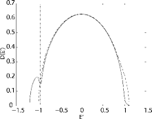
Figure 1: Density of states (DOS) for different temperatures, (a) $k_{B}T=0$, (b) $k_{B}T=5\text{x}10^{-3}W$, (c) $k_{B}T=7.99\text{x}10^{-3}W$ and (d) $k_{B}T=8.1\text{x}10^{-3}W$, when $x=0.053$, $E_{NM}=E_{M}=0$, $\mu_{B}B=0$, $J_{pd}=0.4W$ and $\text{p}=0.8x$. The full line curve is the DOS for the spin down carrier, the dashed one is the DOS for the spin up and the vertical line shows the Fermi level. One can see that the density of states is, relative to a nonmagnetic system, a strong function of temperature.

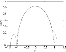
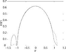
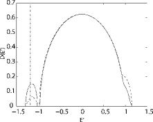
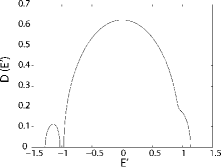
Figure 2: Density of states (DOS) for different temperatures, (a) $k_{B}T=0$, (b) $k_{B}T=2.5\text{x}10^{-3}W$, (c) $k_{B}T=4.5\text{x}10^{-3}W$ and (d) $k_{B}T=5.4\text{x}10^{-3}W$, when $x=0.053$, $E_{NM}=E_{M}=0$, $\mu_{B}B=0$, $J_{pd}=0.5W$ and $\text{p}=0.3x$. The solid line curve is the DOS for the spin down carrier, the dashed one is the DOS for the spin up and the vertical line shows the Fermi level. One can see that the density of states is, relative to a nonmagnetic system, a strong function of temperature.

The diagrams shows the evolution of the spin dependent density of states as a function of temperature for four different temperatures in each figure. The temperature is measured in units of the bandwidth W. In Fig. 1 and 2 one can no longer see the spin-splitting. The position of the Fermi level is also shown. Note that all energy parameters are normalized by $W$ ($E^{\prime}=E/W$). From Fig. 1 and Fig. 2, one can see that when the magnetic coupling $J_{pd}$ is very small, the split band disappears (see Ref. Arsenault, 2006 for details at low $J_{pd}$), whereas in the opposite limit, the spin bands split off and a pseudo gap-appears.

Figure. 3 shows the resistivity in zero $B$ field as a function of temperature with p as a parameter. Results for two values of $J_{pd}$ are presented. The results for lower $J_{pd}$ than $0.35W$ are similar to Fig. 3Arsenault (2006).

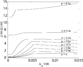
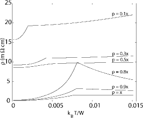
Figure 3: Resistivity as a function of temperature for two $J_{pd}$, (a) $J_{pd}=0.35W$ and (b) $J_{pd}=0.4W$ for an impurity concentration $x=0.053$, $E_{NM}=E_{M}=0$ and $\mu_{B}B=0$, for two values of $J_{pd}$ , with p as a parameter.

When the impurity bands completely splits from the valence band ( for example for $J_{pd}=0.5W$ ), the qualitative behavior changes, as there are now two well defined bands, above and below the Fermi level (impurity and valence) separated by a gap (see Fig. 2 above and Ref. Arsenault, 2006 ). At high hole concentration ($\text{p}\geq 0.8x$), the system is metallic and resistance increases with spin disorder, at first rapidly, and then decreases again above $T_{c}$. This is intuitively to be expected because at first, as temperature increases, the disorder increases, and then in the paramagnetic phase, thermal broadening overcomes the potential scattering disorder and the lifetime averages out. We should remember that in the simplest Boltzmann approach the conductivity is given by

$$\sigma_{xx}=e^{2}\sum_{s}\int D_{s}(E)\left(-\frac{\partial f(E)}{\partial E}\right)v_{s}^{2}(E)\tau_{s}(E)dE$$ (46)

and at low temperatures, depending on the product of the scattering time and the density of states at the Fermi level. In an alloy, either quantity can change with $B$ and $T$ and determine the conductivity. Above $T_{c}$ the spin splitting disappears and the quantities involved are, in the absence of charged impurity scattering, only weak functions of temperature. At very low hole concentration, the Fermi level is in a region of small density of states where we expect localization. However, CPA is a mean field method and does not produce localization. Even though the resistance increases with decreasing density of states at the Fermi level, the conduction process continues to be band conduction albeit with short relaxation time. Even if the mean free path reaches the lattice spacing (random phase limit), the conductivity is still far greater than hopping conductivity between localized levelsAllen et al. (2004). The effect of temperature on resistivity above $T_{c}$ is not too significant in the non-localized intermediate cases. The temperature dependence of the resistance is, in general, a complex interplay of density of states, velocity and relaxation time (imaginary part of the self-energy). The temperature induced lowering of the charged impurity screening length (see Eq. (VII) to Eq. (51)) is not included here. In this range of exchange coupling, $J_{pd}$ does not seem to strongly influence the structure of the resistivity versus $T$ curves but does change their magnitude. In Fig. 3, for $\text{p}=0.1x$, a low carrier concentration, one may see that the resistance increases with $J_{pd}$. In contrast, in the high hole concentration limit $\text{p}=x$, there is only a relatively weak variation of resistance behavior with $J_{pd}$. The complex but regular behavior of resistance with temperature is a manifestation of Eq. (46), reflecting the different elements which determine the value of resistance for a given set of parameters.

Figure 4 shows the resistivity at one temperature, as a function of impurity concentration for varying degrees of hole doping.

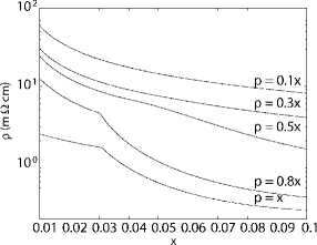
Figure 4: Resistivity as a function of impurity concentration $x$, for varying degrees of hole doping. The others parameters are $J_{pd}=0.35W$, $E_{NM}=E_{M}=0$, $k_{B}T=3.5\text{x}10^{-3}W$ and $\mu_{B}B=0$.

The results of Fig. 3 and Fig. 4 are based on the spin scattering model with no additional potential scattering terms, and no electron-phonon interaction. A fit to experimental data must take these other mechanisms into account as well. Thus, the complete CPA self-energy should include other sources of random potential scattering (nonzero values of $E_{NM}$, $E_{M}$), in particular, the charged impurity scattering terms discussed below. We should also add, when necessary, the electron-phonon self-energy $\Sigma_{ep}(E)$. The imaginary part of the charged impurity self-energy will contribute another source of temperature dependent lifetime broadening, and the real part will enter the density of states.

Figure 5 shows the resistivity as a function of temperature for various magnetic fields, for one value of $x$, p, and $J_{pd}$, and again with $E_{M}=E_{NM}=0$.

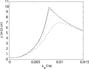
Figure 5: Resistivity as a function of temperature for various magnetic fields. Others parameters are $x=0.053$, $E_{NM}=E_{M}=0$, $J_{pd}=0.4W$ and $\text{p}=0.8x$. The solid line is the zero field result, the dashed line is for $\mu_{B}B=1\text{x}10^{-5}W$, the dotted line is for $\mu_{B}B=1\text{x}10^{-4}W$ and the dashed-dotted line is for $\mu_{B}B=3\text{x}10^{-4}W$.

Apart from very low and very high temperature, increasing magnetic field decreases the resistivity, by favoring the alignment of the impurity spins. The magnetic field also eliminates the sharp metal-insulator transition around $T_{c}$, replacing it with a smooth transition.

Figure 6 shows the relative magnetoresistivity defined by

$$MR\equiv\frac{\rho_{xx}(B^{ext})-\rho_{xx}(B^{ext}=0)}{\rho_{xx}(B^{ext}=0)}$$ (47)

as a function of $B$, for various value of $T$.

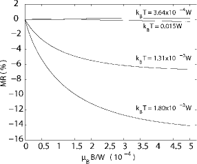
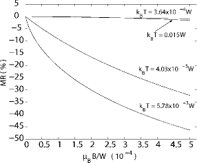
Figure 6: Relative magnetoresistivity for two carrier concentration, (a) $\text{p}=0.1x$ and (b) $\text{p}=0.8x$, for impurity concentration $x=0.053$, $E_{NM}=E_{M}=0$ and $J_{pd}=0.35W$, with $T$ as a parameter.

The overall trend in this exclusively spin scattering model is strong negative magnetoresistivity, as one would expect, since increasing Mn spin alignment reduces disorder, and thus reduces the scattering lifetime, and no other source of scattering are considered. However, lifetime is not the only quantity entering the conductivity. As shown in Eq. (46), the density of states $D(E_{F})$ at $E_{F}$ also plays an important role. There are also regimes of positive magnetoresistivity. From Fig. 6, we see that it is also possible for the resistance to increase with $B$ at low $T$ when the hole density is very low. This is probably because in this limit, the density of states at the Fermi level decreases with magnetic field and this effect is stronger than the concomitant increase of the carrier lifetime due to the suppression of spin disorder with $B$. But we also know that for low concentrations, when the Fermi level is at the band edge or in the region of localized states, other changes arise which are not due to spin disorder scattering and which require another approach which is based on localization. In the hopping regime, not describable by CPA, the magnetic field can, for example, squeeze the localized wavefunctions and increases resistance by reducing overlap. But it also shifts the energy and the mobility edge such as to reduce resistanceMovaghar and Roth (1994). When the calculated resistance is high and when the Fermi level is in a region of small density of states $<~{}10^{19}/\text{cm}^{3}\text{eV}$, we should therefore not trust the CPA, which gives a good description only of the metallic regime.

VI.2 Hall effect

By definition, the Hall resistance is given by

$$\rho_{yx}=\frac{-\text{Re}\Big{\{}\sigma_{yx}\Big{\}}}{\text{Re}\Big{\{}\sigma_{xx}\Big{\}}^{2}-\text{Re}\Big{\{}\sigma_{yx}\Big{\}}\text{Re}\Big{\{}\sigma_{xy}\Big{\}}}.$$ (48)

Equation (48) being a general definition, the normal and the anomalous spin-orbit generated Hall resistance are included.

In the CPA, the sign of the normal Hall effect is not determined by a simple relationship, but depends on the dispersion of the lattice and the behavior of the real part of the Green’s function at the Fermi levelArsenault (2006); Movaghar and Cochrane (1991a). A full analytical analysis of the CPA Hall sign is beyond the scope of this article but we can state that there is no simple rule. The closest to one is that $R_{H}$ is electron-like when the density of states increases with energy and hole-like when it decreases. In the approximation of skew scattering, the sign of the anomalous effect follows the sign of the normal effect as long as the carriers at the Fermi level are polarized in the same direction as the total magnetization. This is true here, as can be seen from Fig. 1. The majority spin band at the Fermi level has the same sign as the overall magnetization, which is dominated by the localized spins. Thus, in the phase addition approximation of Eq. (33), in order to get the right sign, it is essential to keep the correlation between spin and energy. The decoupling of the spin magnetization out of the Kubo formula can give rise to the wrong sign. Here, the overall polarization, found using Eq. (41), is opposite to the direction of the field as it should be. We correct for this effect by assuming that $\langle\sigma_{z}\rangle$ is in the same direction as the overall magnetization.

Figure 7 shows, for a selected class of parameters, the overall behavior of the Hall resistivity in the skew spin scattering model.

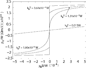
Figure 7: Hall resistivity as a function of the applied magnetic field for two carrier concentration, (a) $\text{p}=0.1x$ and (b) $\text{p}=0.8x$, for an impurity fraction $x=0.053$, $E_{NM}=EM=0$ and $J_{pd}=0.35W$, with $T$ as a parameter

In order to explain the experimental data we need $\frac{\hbar}{\tau_{s}}\frac{1}{2t}=0.2$, which means that the skew scattering energy has to be 0.4 times the tight binding overlap. This is a very (too) strongly enhanced skew scattering rate. It suggests that the correct interpretation of the AHE in GaMnAs is most likely the intrinsic mechanism proposed by Sinova et al.Sinova et al. (2004). In this work, the AHE is due to the intrinsic spin-orbit field, and relies on the multiple band nature of this class of semiconductors. The usual simple nearest neighbor tight-binding model only gives a skew scattering contribution. The universality and order of magnitude of the AHE in ferromagnets suggests that the intrinsic process dominates in most cases.

At high temperature, the magnetism disappears. The normal Hall conduction, linear in $B$ field, is recovered (see the $k_{B}T=0.015W$ results Fig. 7 and Fig. 7). Note that for simplicity of notation, we refer to the applied field in the figure as B, even if it was defined otherwise previously.

VII Experimental relevance

Figure 8 shows results of the CPA calculations for the three transport parameters: resistance, magnetoresistance and Hall effect in a range of parameters for which a behavior close to the ones observed experimentally by RuzmetovRuzmetov et al. (2004) and Ohno et al.Ohno et al. (1992) is observed. We have added a constant contribution to the resistivity so that the relative change in resistivity, such as discussed in connection with Fig. 3, between $T_{c}$ and $T=0$ is of the same order of magnitude as observed in experiment.

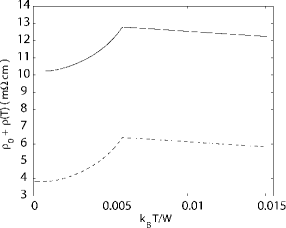
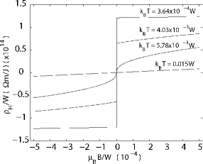
Figure 8: Transport coefficients which can be directly compared to experiment, (a) $\rho=\rho_{0}+\rho(T)$, (b) $MR(B)$ and (c) $\rho_{H}(B)$, for $E_{NM}=E_{M}=0$, $J_{pd}=0.35W$ and $\text{p}=0.8x$. Two possible constant contributions are shown in (a), the solid line curve has $\rho_{0}=10$m$\Omega$cm and the dashed line curve has $\rho_{0}=3.6$m$\Omega$cm

The constant term is chosen to be of the same order of magnitude as the spin scattering rate. The qualitative temperature structure is satisfactory in the ’metallic regime’ of the material, but because we have neglected the charged impurity scattering, we are underestimating the temperature drop of the resistivity with temperature, at higher temperatures. The latter is due to a reduction in screening length when the density of states at the Fermi level increases, (see Eq. (51)). Figure 8 also illustrates the strong temperature dependence of the magnetoresistance, which reaches 40 to 50$\%$ at $k_{B}T\sim 0.0057W$ (this is $\sim 60K$ for $W=1eV$), and how it is intimately connected to the magnetic order as observed experimentally. For an even clearer picture of the connection see Fig. 5. The reader should note that Van Esch et al.Van Esch et al. (1997) have observed magnetoresistances of $\sim$ 500% at $T=4K$ and 50% at $T=20K$ in their more resistive samples with $\rho\sim 1\Omega$/cm. In this sample the magnetization dropped by $\sim 100\%$ between $4K$ and $20K$.

Hwang and Das SarmaHwang and Das Sarma (2005) and Lopez-Sancho and BreyLopez-Sancho and Brey (2003) quite rightly pointed out that when charged impurities are present, they will normally dominate the scattering rate and the temperature dependence of resistance in a wide range of parameters. They then decided to use two different conductivity models for the transport in Mn doped GaAs, one to explain the temperature dependence of the resistance which emphasizes charged impurity scattering, and one for the magnetoresistance which emphasizes spin scattering. We believe this is not necessary. It is enough to add the configurationally averaged charged impurity self-energy to the basis band dispersion $\varepsilon_{\textbf{k}s}\rightarrow\varepsilon_{\textbf{k}s}+\Sigma_{\textbf{k}s}$, and then to neglect, in the simplest limit, the real part of the impurity scattering self-energy $\Sigma_{\textbf{k}s}$. Thus we replace the CPA self-energy, $\Sigma_{s}$, which appears in Eq. (16), by

$$\text{Im}\Big{\{}\Sigma_{s}(E)\Big{\}}+\text{Im}\Big{\{}\Sigma_{\textbf{k}s}(E)\Big{\}}=\text{Im}\Big{\{}\Sigma_{s}(E)\Big{\}}+$$

$$\eta\int d\textbf{k}^{\prime}\left(\frac{1}{2\pi}\right)^{3}\left|V_{\textbf{k}-\textbf{k}^{\prime}}\right|^{2}(1-\cos\theta_{\textbf{k}-\textbf{k}^{\prime}})\delta\Big{(}E-\varepsilon_{\textbf{k}^{\prime}s}\Big{)},$$

where $\eta=\frac{2\pi}{\hbar}N_{i}$, with $N_{i}$ the impurity concentration, and

$$V_{\textbf{k}-\textbf{k}^{\prime}}=\frac{4\pi Z_{imp}e^{2}}{\varepsilon\varepsilon_{0}\left|\textbf{k}-\textbf{k}^{\prime}\right|^{2}}\frac{1}{1+\left(q_{sc}/\left|\textbf{k}-\textbf{k}^{\prime}\right|\right)^{2}}.$$ (50)

In Eq. (50), $Z_{imp}$ is the impurity charge number, and

$$q_{sc}^{2}=4\pi e^{2}\sum_{s}\int dED_{s}(E)\left(-\frac{\partial f(E)}{\partial E}\right)$$ (51)

is the inverse screening length. Since the results of Section VI show that $D_{s}(E)$ at the Fermi level change with temperature and field, the screening length will change as well. Note that usually, in Boltzmann transport, one does not take into account the effect of the real part of the self-energy (the imaginary part gives the scattering) on the actual band structure because the concentration of dopants is low. Here the concentration is not low. The real part should in principle, modify the band gap and effective masses and can be included in our formalism.

We agree with Hwang and Das SarmaHwang and Das Sarma (2005) that the complete problem in parameter space is enormously complex. In effect, we should want the impurity scattering to only represent an additional self-consistent, density of states dependent, lifetime process. A fully self-consistent Coulomb potential/spin multiband CPA is far too complex, and of little value. In addition, the CPA band theory cannot account for the hopping regime, as pointed out in the previous section.

VIII The problem of the intrinsic and extrinsic Hall effect

In the Kane-Luttinger theory of Jungwirth et al.Jungwirth et al. (2006), the Mn dopants only cause a lifetime broadening and no change to the Kane-Bloch bandstructure. In this formalism, the intrinsic spin-orbit interaction is Bloch invariant and only causes band mixing. All disorder is treated only as a lifetime effect. This is not so in the CPA where the dopant scattering causes a substantial renormalization of the bandstructure via the real part of the self-energy and indeed gives an explanation of the magnetism. The spin-orbit coupling produces new terms in the Hamiltonian which allow the electrons jumping or tunneling from one site to the next site to experience the electric field of the neighboring atoms. The 3-site processes we invoke are not normally included in the tight-binding modeling of semiconductors. They represent only small modifications of the bandstructure, much smaller than the on-site spin-orbit admixture. The anomalous Hall mechanism in one band tight-binding is basically one of ”skew scattering”, except that the jump is always from orbit to orbit, and the effective magnetic field can only come from another $3^{rd}$ site. We have seen that the one band TB description is inadequate to describe the AHE in DMS. On the other hand, the multiple band Kane and/or Kohn-LuttingerKohn and Luttinger (1957) approach seems to work well. It gives the right order of magnitude with an intrinsic AHE. This suggests that a TB modeling of the AHE must include the multiple band aspect and at least a second nearest neighbor overlap. Since, for example, a five percent GaMnAs alloy cannot have a true Bloch band structure, in the orbital description, it is the short range many orbital aspect which must give rise to the intrinsic AHE.

IX Conclusion

We have presented a CPA theory which could explain the magnetism in Mn doped semiconductors in the metallic regime and allows one to calculate the transport parameters. The numerical evaluation of resistance, magnetoresistance and Hall coefficient, normal and anomalous, show that the overall trends observed experimentally are reproduced by the CPA. The power of the method lies in its simplicity. All the information is contained in a spin and energy dependent self-energy $\Sigma_{s}(E)$. In good approximation, we may add the effect of the charged impurity and electron-phonon lifetime corrections to the calculated CPA self-energy. Of the two, the first is the most important addition because it explains why the experimental resistance decreases at high temperatures (in general more strongly than shown in Fig. 8), when the ferromagnetism has reduced to paramagnetism, and spin-disorder scattering should have reached its highest value. The ”small” resistance drop at high temperature seen in Fig. 8 is due to CPA bandstructure renormalization. The CPA and $t$-matrix methods can be extended to treat magnetic clusters and evaluate effective localized spin-spin coupling mediated by the band.

We have also demonstrated how to include charged impurity scattering within the same formalism. The central aim of this paper was to achieve an understanding of the important mechanism which determines the conductivity behavior. For this purpose, we have used a one-band approach which is adequate to understand the conductivity. For optical properties and the intrinsic AHE, the many band aspects are essential.

The AHE has been modeled as an extrinsic effect in the framework of skew scattering. We did this using the tight-binding language. The intrinsic AHE, as invoked by Jungwirth et al.Jungwirth et al. (2006), cannot be derived using a nearest neighbor TB formalism, and it is not clear how to recover it in the TB formalism. The problematic of the intrinsic AHE and the TB model is an interesting one. It should be re-examined in detail because so far, the nearest neighbor tight-binding methods have proved useful as bandstructure descriptions of semiconductors.