Optimized Cooper pair pumps

Abstract

In adiabatic Cooper pair pumps, operated by means of gate voltage modulation only, the quantization of the pumped charge during a cycle is limited due to the quantum coherence of the macroscopic superconducting wave function. In this work we show that it is possible to obtain very accurate pumps in the non-adiabatic regime by a suitable choice of the shape of the gate voltage pulses. We determine the shape of these pulses by applying quantum optimal control theory to this problem. In the optimal case the error, with respect to the quantized value, can be as small as of the order of $10^{-6}e$: the error is reduced by up to five orders of magnitude with respect to the adiabatic pumping. In order to test the experimental feasibility of this approach we consider the effect of charge noise and the deformations of the optimal pulse shapes on the accuracy of the pump. Charge noise is assumed to be induced by random background charges in the substrate, responsible for the observed $1/f$ noise. Inaccuracies in the pulse shaping are described by assuming a finite bandwidth for the pulse generator. In realistic cases the error increases at most of one order of magnitude as compared to the optimal case. Our results are promising for the realization of accurate and fast superconducting pumps.

I Introduction

A dc current can be generated in a mesoscopic circuit connected to two electrodes even in the absence of a bias voltage if a set of external parameters, e.g. gate voltages, are changed periodically in time thouless83 . This mechanism is known as charge pumping. If the external parameters are changed slowly as compared to the typical time scales of the system the pumping is adiabatic. In this case the charge pumped after one cycle does not depend on the detailed timing of the cycle, but only on its geometrical properties. Charge pumping can be realized in a variety of different situations. In systems consisting of mesoscopic phase-coherent conductors parametric pumping can be achieved through a periodic modulation of the phases of the scattering matrix. This regime has been studied extensively both for metallic conductors, see e.g. Refs. brouwer98, ; zhou99, ; makhlin01, ; moskalets02a, ; moskalets02b, ; entin02, and hybrid systems wang01 ; blaauboer02 ; taddei04 containing superconducting terminals. In the opposite regime of systems consisting of quantum dots connected through tunnel junctions, charge pumping is achieved by the periodic modulation of the Coulomb blockade SCT92 . In this case phase coherence is irrelevant and the number of electrons transfered per cycle is approximately quantized: the generated current $I$ is related to the frequency of cycle $f$ via $I\sim(ne)f$, where $n$ is the number of electrons transfered in each cycle and $e$ is the electron charge. Experimental evidence for parametric charge pumping in normal metallic systems has been demonstrated for the first time in Refs. kouwenhoven91, ; pothier92, .

The situation is radically different if superconducting islands are considered. Here at low temperatures pumping is due to the transport of Cooper pairs geerligs91 ; niskanen05 . A Cooper pair pump can be realized by an array of Josephson junctions connected to two superconducting reservoirs, kept at a fixed phase bias $\varphi$ footnote . In this case, even in those situations where pumping is associated to a periodic modulation of the Coulomb blockade, superconducting phase coherence is fundamental pekola99 ; niskanen03 . Moreover, in addition to the dependence of the pumped charge on the characteristics of the cycle, in superconducting pumps there is a dependence on the superconducting phase difference between the reservoirs. The geometric nature of the pumped charge has been analyzed both in the Abelian aunola03 ; governale05 ; mottonen06 ; leone07 and non-Abelian brosco07 cases thus opening the possibility to experimentally detect geometric phases in superconducting nanocircuits falci00 ; leek07 . Indeed an experimental detection of the Berry phase by means of Cooper pair pumping has recently been reported mottonen07 .

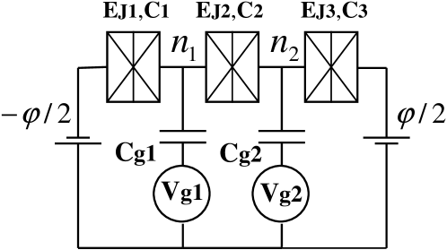
Figure 1: Schematic drawing of a Cooper pair pump consisting of three Josephson junctions and two gated Cooper pair boxes. $C_{i}$ and $E_{Ji}$ are the capacitances and Josephson energies of the junctions. $C_{gi}$ and $V_{gi}$ are gate capacitances and voltages, $\varphi$ is the overall phase difference. By a proper modulation of the gate voltages a given charge is moved from, say, the left to the right electrode. In general the pumped charge will depend on the modulation shape and on the phase difference $\varphi$. In the protocol considered here the dependence on $\varphi$ is absent.

In addition to the importance of addressing fundamental questions related to the quantum mechanical behavior of macroscopic systems, accurate charge pumping can be used for metrological purposes. In the case of single-electron pumps the transfered charge, at frequency $f$ of a few MHz, has reached such an accuracy (uncertainty of $10^{-8}$) to make a new metrological standard of capacitance possible keller96 ; keller98 ; keller99 . By pumping a certain number of electrons onto a capacitor, and measuring the resulting voltage, one can measure capacities of the order of 1pF. On the contrary, the frequencies, and consequently the current intensities, in single-electron pumps has not been sufficiently high for setting a standard of current. A superconducting Cooper pair pump, in principle, would allow for higher frequencies although several effects such as Landau-Zener tunneling, supercurrent leakage through the pump, and coherent corrections (which are of crucial importance to reveal geometric phases) would lead to all sorts of inaccuracies in Cooper pair pumping. Some works have been done to achieve more accurate pumping in adiabatic regime by optimizing the design of the pump niskanen03 ; cholascinski07 ; leone07 . In this paper we follow a different approach. We will design very accurate Cooper pair pumps by optimizing the pulse shapes of the gate voltages during the cycle. Most importantly we are not bound to work in the adiabatic limit therefore increasing, at the same time, both the accuracy and the frequency of operation. The theoretical framework which will apply to achieve this goal is that of optimal control theory peirce88 ; borzi002 ; sklarz002 ; calarco04 . This approach was successfully applied to superconducting qubits to improve one- and two-qubit gates sporl07 ; montangero07 and it was shown that it can help in reducing the error in the gate operation by several order of magnitudes. As we will describe in the rest of the paper, optimal control is also helpful in the case of Cooper pair pumping where, for the case we consider, the error is reduced up to five orders of magnitude.

The paper is organized as follows. In the next Section we will describe the model for the Cooper pair pump used in the rest of the paper. We will then give (Sec. III) a brief introduction to the optimal control algorithm employed in this work. In Sec. IV we present the results obtained for our non adiabatic optimal pump. After having discussed the achieved accuracy (Sec. IV.1) we analyze in details the effect of possible imperfections in the pulse shapes (Sec. IV.2), the effect of noise (Sec. IV.3), as well as the effect of unavoidable variations in charging and Josephson energy from junction to junction (Sec. IV.4), in order to test the robustness of the pump. The last Section is devoted to the conclusions and to a comparison with other proposals to realize accurate pumps.

II The Cooper pair pump

The three-junction Cooper pair pump considered in the paper is shown in Fig. 1. It consists of an array of three Josephson junctions with two gated islands; $E_{Ji}$ and $C_{i}$ are, respectively, Josephson energy and capacity of $i$th junction, while $C_{gi}$ and $V_{gi}$ are, respectively, gate capacitance and gate voltage applied on the $i$th island. The number of extra Cooper pairs on the $i$th island is denoted with $n_{i}$ and $\varphi$ is the overall phase difference between the two superconducting electrodes. In the case of a uniform array, which we consider here, the Hamiltonian, in the basis of charge eigenstates $|\stackrel{{\scriptstyle\rightarrow}}{{n}}\rangle$, is given by pekola99

$$H=\sum_{\stackrel{{\scriptstyle\rightarrow}}{{n}}}\left\{\frac{2}{3}E_{C}\left[(n_{1}-q_{1})^{2}+(n_{2}-q_{2})^{2}+(n_{1}-q_{1})(n_{2}-q_{2})\right]|\stackrel{{\scriptstyle\rightarrow}}{{n}}\rangle\langle\stackrel{{\scriptstyle\rightarrow}}{{n}}|-\frac{E_{J}}{2}\sum^{3}_{k=1}(e^{i\frac{\varphi}{3}}|\stackrel{{\scriptstyle\rightarrow}}{{n}}+\stackrel{{\scriptstyle\rightarrow}}{{\delta_{k}}}><\stackrel{{\scriptstyle\rightarrow}}{{n}}|+h.c.)\right\}$$ (1)

In this equation $\stackrel{{\scriptstyle\rightarrow}}{{n}}=(n_{1},n_{2})$ and $\stackrel{{\scriptstyle\rightarrow}}{{q}}=(q_{1},q_{2})$ specify, respectively, the number of Cooper pairs on each island and the normalized gate charges $(q_{k}=-C_{g,k}V_{g,k}/(2e))$. Tunneling of one Cooper pair through the $k$th junction changes the number of pairs on $k$th and $(k-1)$th island, so that the only non-zero components of $\stackrel{{\scriptstyle\rightarrow}}{{\delta_{k}}}$ are $(\stackrel{{\scriptstyle\rightarrow}}{{\delta_{k}}})_{k}=1$ and $(\stackrel{{\scriptstyle\rightarrow}}{{\delta_{k}}})_{k-1}=-1$. Moreover the forward (backward) tunneling of one pair through each junction is related to a $\frac{\varphi}{3}$ ($-\frac{\varphi}{3}$) phase difference. The pump operates in the charging limit, i.e. $E_{J}\ll E_{C}$.

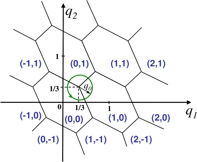
Figure 2: (Color on line) The stability diagram of a three-junction Cooper pair pump in the $(q_{1},q_{2})$ space. Each hexagon corresponds to a given charge (eigen)state (for $E_{J}=0$) of the system $(n_{1},n_{2})$. In the adiabatic regime charge is pumped when the gate charges are varied along, for example, the circular path with radius $q_{0}$ centered at the degeneracy point ($q_{1}=q_{2}=1/3$).

As discussed in Ref. pekola99, the Cooper pair pump is operated by changing periodically in time the two gate charges $q_{1}$ and $q_{2}$.

It is useful to first analyze the case in which the pump is driven adiabatically. In this case the time dependence of the gate charge is not important, what matters is the path which is followed in the parameter space. As was discussed extensively in the past (see e.g. Ref. geerligs91, ; pekola99, ) it is important that the cycle encloses the triple point degeneracy ($q_{1}=q_{2}=1/3$) in the stability diagram as described in Fig.2. The various regions in Fig.2 indicate the corresponding ground state of the charging part of the Hamiltonian. After a cycle, for example the one indicated in the figure, the state of the pump goes back to its initial situation but (approximately) one Cooper pair has been transferred through the system. As it has been discussed in pekola99 , this pump does not lead to a sufficient quantization accuracy: the error scales as $E_{J}/E_{C}$. A smaller error can be achieved either by increasing the number of junctions or by pumping by means of gate voltage and flux modulation as in the Cooper pair sluice niskanen03 .

In the present work we take a different approach to optimize the pump. Our proposed device operates in the non-adiabatic limit, in which the time dependence of the pulses is important. In order to have an accurate pump we will then optimize the pulse shapes by means of quantum optimal control (see next Section). These ingredients allow to construct a fast and accurate Cooper pair pump.

As we will show in the next section, in order to use the quantum optimal control, one needs to have a desired final state differing from the initial state and at least one parameter as a control in the Hamiltonian of the system. Since in pumping the initial and final states of the system are the same apart from a phase we introduce a new quantum number, the counter $|m\rangle$. This counter is a passive detector which clicks each time a Cooper pair goes through the junction where the counter is set. In the following we assume that the counter is placed in the last junction of the array, therefore if one pair passes this junction from left (right) to right (left) the counter will change by 1 ($-1$). We emphasize that the counter considered is merely a fictitious element which we use to compute the pumped charge. No back action can be expected since we are not describing a physical detector. If one denotes the state of the array by $|\Phi(t)\rangle$ and the state of the counter by $|m\rangle$, where $m=0,\pm 1,\pm 2...$, the state of the system will be $|\Phi(t)\rangle\otimes|m\rangle$. In the Hilbert space of charge states plus the counter index the Hamiltonian of a three-junction uniform pump has the following form:

$$\cal H = \frac{2}{3}E_{C}\sum_{m,\stackrel{{\scriptstyle\rightarrow}}{{n}}}\left[(n_{1}-q_{1})^{2}+(n_{2}-q_{2})^{2}+(n_{1}-q_{1})(n_{2}-q_{2})\right]|\stackrel{{\scriptstyle\rightarrow}}{{n}},m\rangle\langle\stackrel{{\scriptstyle\rightarrow}}{{n}},m|$$ (2)

$$- \frac{1}{2}E_{J}\sum_{m,\stackrel{{\scriptstyle\rightarrow}}{{n}}}\left[e^{i\frac{\varphi}{3}}\left(\left|n_{1}+1,n_{2},m\right\rangle+\left|n_{1}-1,n_{2}+1,m\right\rangle+\left|n_{1},n_{2}-1,m+1\right\rangle\right)\left\langle n_{1},n_{2},m\right|+h.c.\right]$$

As it is clear in the Hamiltonian (2), one can change the state of the counter without changing the energy so that all states $|\Phi(t)\rangle\otimes|m\rangle$ with different values of $m$ are degenerate.

III Optimal quantum control

Quantum optimal control algorithms peirce88 ; borzi002 ; sklarz002 ; calarco04 are designed to lead a quantum system with state $|\psi(t)\rangle$ from an initial state $|\psi(0)\rangle=|\psi_{ini}\rangle$ to a target final state $|\psi_{fin}\rangle$ at time $T$ with a good fidelity $\cal F$, where ${\cal F}\equiv|\langle\psi_{fin}|\psi(T)\rangle|^{2}$. The algorithm employed in this work is called immediate feedback control and is guaranteed to give a fidelity improvement at each iteration ref:Sola98 . The procedure is as follows: Assume that $\{u_{j}(t)\}$ is the set of control parameters which the Hamiltonian depends on. First the state of the system $|\psi(t)\rangle$ is evolved in time with the initial condition $|\psi(0)\rangle=|\psi_{ini}\rangle$ and an initial guess $\{u^{(0)}_{j}(t)\}$ for control parameters, giving rise to $|\psi(T)\rangle$ after time $T$. At this point an iterative algorithm starts, aiming at improving the fidelity by adding a correction to control parameters in each step. In the $n$th step of this iterative algorithm

• The auxiliary state $|\chi(T)\rangle\equiv|\psi_{fin}\rangle\langle\psi_{fin}|\psi(T)\rangle$ is evolved backwards in time reaching $|\chi(0)\rangle$. $|\chi(T)$ can be interpreted as the part of the desired final state $|\psi_{fin}\rangle$ which has been reached.

• The states $|\chi(0)\rangle$ and $|\psi(0)\rangle$ are evolved forward in time with control parameters $\{u^{(n)}_{j}(t)\}$ and $\{u^{(n+1)}_{j}(t)\}$, respectively. Here,

  $$u^{(n+1)}_{j}(t)=u^{(n)}_{j}(t)+\frac{2}{\lambda(t)}\Im\left[\langle\chi(t)|\frac{\partial H}{\partial u_{j}(t)}|\psi(t)\rangle\right]$$ (3)

  are updated control parameters and $\lambda(t)$ is a weight function used to fix initial and final conditions on the control parameters.

These two steps are repeated until the desired value of fidelity is obtained.

In this work we will use the described quantum optimal control algorithm to drive the system from the initial state $|\Psi_{ini}\rangle\equiv|G(0)\rangle\otimes|0\rangle$ to the final state $|\Psi_{fin}\rangle\equiv|G(0)\rangle\otimes|1\rangle$, using the Hamiltonian (2) for the time evolution where $|G(0)\rangle$ is the ground state of the Hamiltonian (1) at time $t=0$. The initial state $|G(0)\rangle\otimes|m=0\rangle$ can be achieved by suddenly coupling the array to the electrodes. The normalized gate charges $q_{1}$ and $q_{2}$ will be the control parameters. In all of the numerical simulations we performed we assume $\varphi=0$ so that supercurrent is zero. Moreover, in the adiabatic case and $\varphi=0$ the errors are most severe, so that our settings describe the worst case scenario to test optimal control theory. The expectation value of the counter operator ${\hat{m}}\equiv\sum_{m}m~{}|m\rangle\langle m|$ represents the pumped charge $Q_{p}$ in unit of $2e$. An important measure of the accuracy of the pump is given by the deviation of the pumped charge from the quantized value

$${\cal E}=|1-\frac{Q_{p}}{2e}|\;\;.$$ (4)

In addition, since Cooper pair pumping is a coherent process, it is also interesting to test the accuracy of the optimization protocol by measuring the departure of the final quantum state from the desired one. To this end we also study the fidelity at the end of time evolution

$${\cal F}\equiv|(\langle 1|\otimes\langle G(0)|)|\Psi(T)\rangle|^{2}$$

which measures the overlap between the final state of the array and the ground state $|G(0)\rangle$. In all plots we show the infidelity defined as ${\cal I}=1-{\cal F}$.

IV Optimal Cooper pair pumping

In this section we present our results for the non-adiabatic optimal pump with $\varphi=0$, i. e. when there is no supercurrent. The goal is to achieve a pumped charge as close as possible to $2e$ (we remind that $\varphi=0$ is the case where the error is maximal without optimization).

IV.1 Optimal pumps

Motivated by the adiabatic case, as initial guess for control parameters we choose a circular path in $(q_{1},q_{2})$ space, around the degeneracy point $q_{1}=q_{2}=\frac{1}{3}$ with radius $q_{0}$ described by sinusoidal gate voltages $q_{1}=\frac{1}{3}+q_{0}\cos(2\pi t/T+\theta_{0})$ and $q_{2}=\frac{1}{3}+q_{0}\sin(2\pi t/T+\theta_{0})$, where $\theta_{0}=5\pi/4$. The number of excess charges considered for each box is $n=0,\pm 1$, so that nine lowest charge states of the whole system are allowed to contribute to pumping.

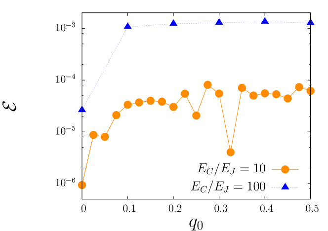
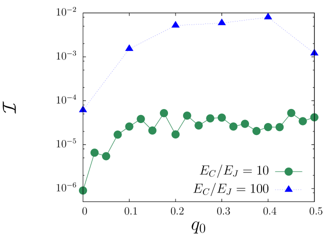
Figure 3: (Color on line) Top panel: Error in pumped charge ${\cal E}$ and Bottom panel: Infidelity ${\cal I}$ after one cycle as a function of radius of circular path $q_{0}$ in $(q_{1},q_{2})$ space, for $E_{C}/E_{J}=10$ and $100$. The vertical axis in both panels is in logarithmic scale. Results are obtained after using the quantum optimal control theory to modify the circular path (at least 200 iterations). $T=30\pi\hbar/E_{J}$ and $\varphi=0$. Numerical error, due to discretization of the time evolution, is at most of the order of $10^{-5}$.

Since the initial paths with radii greater than $1/2$ might involve more states, we take $q_{0}\leq 1/2$. For each given radius, optimal control algorithm modifies the initial path such that the fidelity $\cal F$ after one cycle approaches the value one. In the following we shall mostly focus on an experimentally relevant case and take $E_{C}/E_{J}=10$. In this case in the adiabatic regime the accuracy of the pumped charge is always smaller than fifty percent pekola99 . As shown in Fig. 3, accurate pumping could be achieved with $T=30\pi\hbar/E_{J}$, which is already in the non-adiabatic regime, after at least $200$ iterations. In the top panel of Fig. 3 we plot the error in pumped charge ${\cal E}$ as a function of radius $q_{0}$, while the bottom panel shows the infidelity ${\cal I}$. Both error and infidelity are always less than $10^{-4}$. In Fig. 3 we show also some results for $E_{C}/E_{J}=100$ (triangles), with error and infidelity always smaller than $10^{-2}$. The difference between the accuracy of these two cases is due to the stronger violation of adiabatic condition, $T\gg\hbar E_{C}/E_{J}^{2}$, in the case $E_{C}/E_{J}=100$ compared to $E_{C}/E_{J}=10$. Notice, moreover, that the optimization procedure allows to control directly the fidelity but only indirectly the value of pumped charge so that the behavior of ${\cal I}$ and ${\cal E}$ as a function of $q_{0}$ are not expected to be equal.

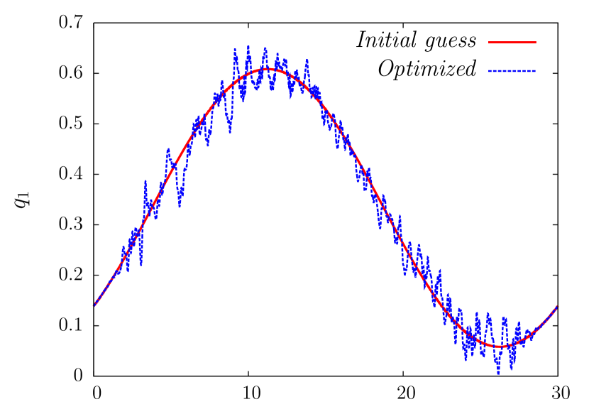
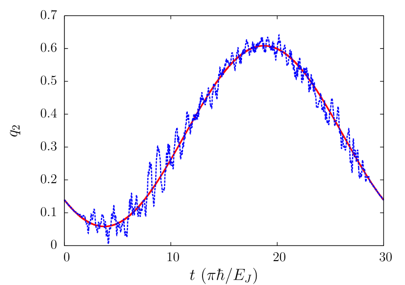
Figure 4: (Color on line) An example of gate voltages $q_{1}$ (top panel) and $q_{2}$ (bottom panel) as a function of time, before and after optimization (200 iterations). The solid red lines correspond to initial circular path with radius $q_{0}=0.275$ around the degeneracy point $q_{1}=q_{2}=1/3$ in $(q_{1},q_{2})$ space. Dotted blue lines are optimized voltages leading to accurate pumping. $T=30\pi\hbar/E_{J}$, $E_{C}/E_{J}=10$ and $\varphi=0$.

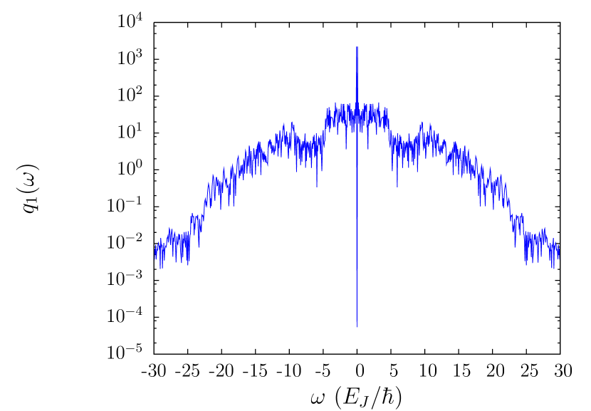
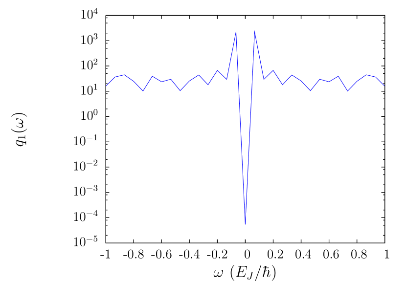
Figure 5: (Color on line) An example of Fourier transform of optimized gate voltage $q_{1}$ (blue curve in the top panel of fig.4). Top panel shows most important harmonics as a function of frequency and few first harmonics are shown in bottom panel. $q_{0}=0.275$, $T=30\pi\hbar/E_{J}$, $E_{C}/E_{J}=10$ and $\varphi=0$.

IV.2 Imperfections in the pulse shapes

It is important to understand to which extent the pulses which optimize the pumping can be realized in experiments. Fig. 4 shows an example ($q_{0}=0.275$) of initial (red line) and optimized (blue dotted line) gate voltages $q_{1}$ (top panel) and $q_{2}$ (bottom panel) after 200 iterations. In the top panel of Fig. 5 we show the Fourier transform $q_{1}(\omega)$ of the optimized gate voltage $q_{1}(t)$ plotted in Fig. 4, while in the bottom panel the same curve is plotted on a smaller range of frequencies. Note that the largest contribution occurs for $\omega=\pm 1/15E_{J}/\hbar$, which is the frequency of the initial sinusoidal gate voltages. In a realistic situation, however, it is very difficult to imagine that all the details of the pulse, encoded in the high frequency components, can be reproduced faithfully. We accounted for imperfections in the pulse shape by introducing a bandwidth parametrized by a high frequency cutoff $\omega_{cutoff}$. In Fig. 6 we show both the error and the infidelity as a function of the bandwidth for three different radii of initial circular path. No changes occur by decreasing $\omega_{cutoff}$ from 100 $E_{J}/\hbar$ until $\omega_{cutoff}\approx 15E_{J}/\hbar$ is reached and at this point a dramatic increase in both error and infidelity occurs which demonstrates the importance of harmonics with frequencies close to this value. Another change in pumped charge and fidelity happens when $\omega_{cutoff}\approx 5E_{J}/\hbar$ is reached. Therefore the most important harmonics for optimizing the gate voltages lie below $\omega=20E_{J}/\hbar$ and there is no need for higher frequencies in order to pump accurately.

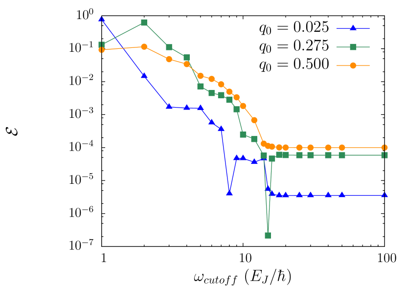
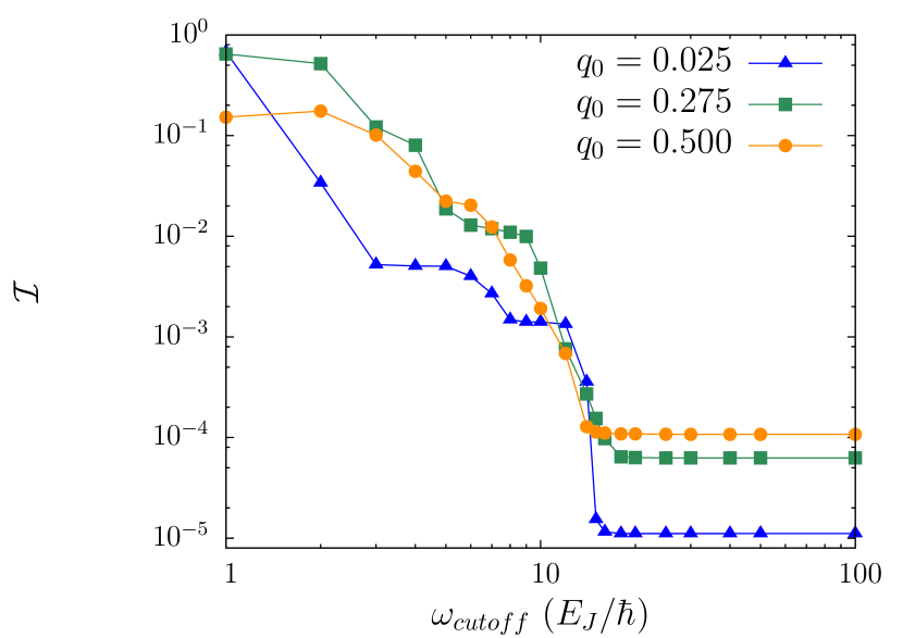
Figure 6: (Color on line) The error $\cal E$ in pumping one Cooper pair in each cycle (top panel) and the infidelity $\cal I$ of ending up to the ground state of the array at the end of cycle (bottom panel), in optimized non-adiabatic case, as a function of the cutoff frequency $\omega_{cutoff}$ of gate voltages. Different curves are related to different radii of circular path in $(q_{1},q_{2})$ space as the initial guess for control parameters in quantum optimal control theory. $E_{C}/E_{J}=10$, $T=30\pi\hbar/E_{J}$ and $\varphi=0$. Numerical error is at most of the order of $10^{-5}$.

IV.3 Effect of noise

We finally discuss the effect of external noise. Since Cooper pair pumping is a coherent process, the presence of an external environment may be disruptive. In Josephson nanocircuits in the charge regime the dominant mechanism of decoherence is $1/f$ noise (see e.g. Ref. ithier05 ). It is important to know whether the pumped charge is stable while optimized gate voltages are affected by noise. Although its understanding is far from complete, $1/f$ noise is believed to originate from two-level fluctuators present in the substrate and/or in the insulation barrier. Several theoretical works have recently studied the effect of $1/f$ noise backgroundcharges . Following current approaches, we model the environment as a superposition of bistable classical fluctuators resulting in an additional random contribution $\delta q_{k}(t)$ to the gate charges after optimization.

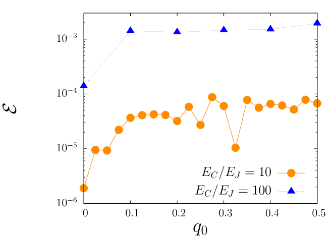
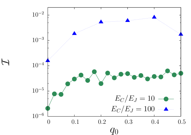
Figure 7: (Color on line) Error in pumped charge ${\cal E}$ (top panel) and infidelity ${\cal I}$ (bottom panel) after one cycle as a function of radius of circular path $q_{0}$ in $(q_{1},q_{2})$ space, for $E_{C}/E_{J}=10$ and $100$, after applying the noise with power spectrum ${\cal S}_{q_{k}}(\omega)={\cal A}/\omega$ and strength ${\cal A}=10^{-5}$ on optimized gate voltages. $T=30\pi\hbar/E_{J}$ and $\varphi=0$. The vertical axis in both panels is in logarithmic scale. Numerical error is at most of the order of $10^{-5}$.

A distribution of switching rates $\gamma$ behaving as $P(\gamma)\propto 1/\gamma$ in a range $[\gamma_{min}:\gamma_{max}]$ results in a noise power spectrum ${\cal S}_{q_{k}}(\omega)=\langle\delta q_{k}(t)\delta q_{k}(0)\rangle_{\omega}\approx\omega^{-1}$. We chose the switching rates such that the $1/f$ part of the spectrum is centered around the typical frequency of the pump. Typically the $1/f$ region extends over two order of magnitudes in $\omega$. We assume that fifty independent fluctuators are coupled weakly to the system and that the charge noise on the two separate gates are uncorrelated. Moreover we averaged the results over fifty different configurations of noise. In Fig. 7 we plot the error $\cal E$ (top panel) and infidelity $\cal I$ (bottom panel), as a function of $q_{0}$, for a strength of noise ${\cal A}=10^{-5}$ (${\cal S}(\omega)={\cal A}/\omega$), which is a typical experimental value. Remarkably, the pumped charge is virtually unaffected by noise: for $E_{C}/E_{J}=10$ the error in the pumped charge and infidelity are still less than $10^{-4}$, which clearly shows the stability against noise. The case $E_{C}/E_{J}=100$ is also stable. To complete the analysis, we plot in Fig. 8 the error in pumped charge (top panel) as well as the infidelity (bottom panel) as a function of $\cal A$ for a few different values of $q_{0}$ (note that both vertical and horizontal axes are in logarithmic scale). For all values of radius $q_{0}$ the accuracy of pumping and fidelity are larger than $90\%$ even under the effect of noise with significant strength ${\cal A}=10^{-3}$, which is a good improvement considering that the accuracy is less than fifty percent in adiabatic regime without noise. More importantly, both ${\cal E}$ and ${\cal I}$ are not increasing up to about ${\cal A}=10^{-5}$.

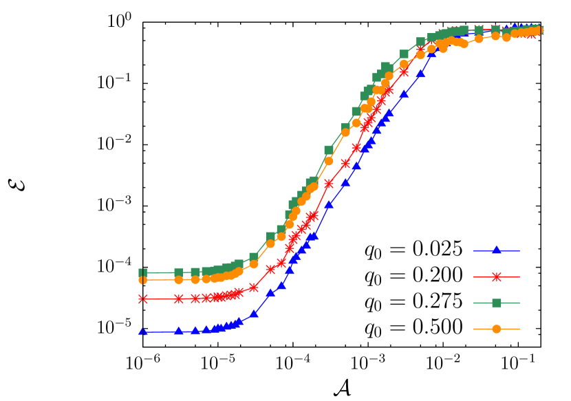
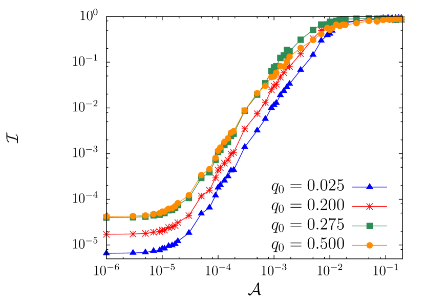
Figure 8: (Color on line) The error $\cal E$ in pumping one Cooper pair in each cycle (top panel) and the infidelity $\cal I$ of ending up to the ground state of the array at the end of cycle (bottom panel), in optimized non-adiabatic case, as a function of the strength of the $1/f$ noise $\cal A$ affecting gate voltages. Different curves are related to different radii of circular path in $(q_{1},q_{2})$ space as the initial guess for control parameters in quantum optimal control theory. $E_{C}/E_{J}=10$, $T=30\pi\hbar/E_{J}$ and $\varphi=0$. Numerical error is at most of the order of $10^{-5}$.

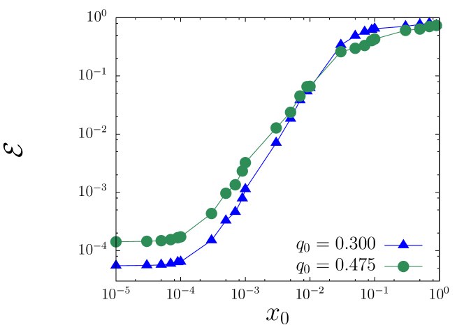
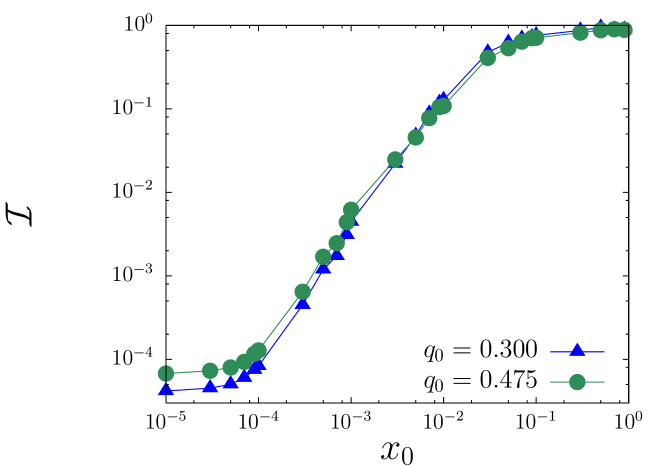
Figure 9: (Color on line) The error $\cal E$ (top panel) and the infidelity $\cal I$ (bottom panel), as a function of the random fraction $x_{0}$ added to the nominal $E_{C}$ and $E_{J}$. Optimized pulses obtained for uniform array are used to calculate pumped charge and fidelity. $E_{C}/E_{J}=10$, $T=30\pi\hbar/E_{J}$ and $\varphi=0$. Numerical error is at most of the order of $10^{-5}$.

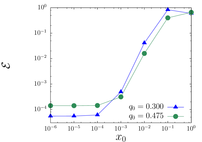
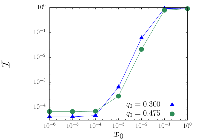
Figure 10: (Color on line) The error $\cal E$ (top panel) and the infidelity $\cal I$ (bottom panel), as a function of the weight $x_{0}$ of the random Hamiltonian added to the uniform Hamiltonian. Optimized pulses obtained from non-perturbed Hamiltonian are used to calculate pumped charge and fidelity. $E_{C}/E_{J}=10$, $T=30\pi\hbar/E_{J}$ and $\varphi=0$. Numerical error is at most of the order of $10^{-5}$.

IV.4 Imperfections in the pump

Up to now we have assumed the ideal situation in which the parameters of the pump are known. In this section we address the effect of imperfections arising when such parameters are known only up to a given uncertainty from a uniform array. More precisely, we estimate how error in pumped charge and infidelity increase, as a function of the extent of the uncertainty, by evolving the system using the optimized pulse shapes calculated for the uniform array. To assess this issue we have implemented such an uncertainty on the parameters with two methods. In the first one we add to the nominal $E_{C}$ and $E_{J}$, of a uniform array, a random fraction $x$ taken in the range $[-x_{0},x_{0}]$. In Fig. 9 we plot error and infidelity, respectively, averaged over 50 configurations as a function of $x_{0}$ for $E_{C}=10E_{J}$, for $q_{0}=0.300$ and $q_{0}=0.475$. In the second method we perturb the uniform Hamiltonian by adding to it a weighted random matrix. In Fig. 10 we plot error and infidelity, respectively, as a function of the weight $x_{0}$ for $E_{C}=10E_{J}$ and for two values of $q_{0}$. Both methods show that no increase of infidelity and epsilon is found up to a fraction (or a weight) of the order of $10^{-4}$. Finally, we emphasize that we have always assumed a uniform array simply for the sake of definiteness. Indeed, in the case of non-uniformity of the parameters, as long as they are known, the pulse optimization can always be performed. Of course, the shape of the final optimized pulses would be different, with respect to the uniform situation, depending on the extent of the non-uniformity.

V Conclusion

In this paper we presented a proposal for realizing fast and accurate Cooper pair pumps. The idea was to use a conventional gate-based Cooper pair pump with optimized pulse shapes. This pump operates in the non-adiabatic regime and, as we showed, can achieve a high accuracy. Numerical results after using the optimal control theory were presented demonstrating that pumped charge is accurate and stable against the noise applied on gate voltages and uncertainty in charging and Josephson energy. Moreover all important harmonics contributing to optimized gate voltages have frequencies less than few $E_{J}/\hbar$. The simple design of the pump, the short time scales of operation and the stability against noise are advantages which make it worthy to think of the quantum optimal control theory as a powerful tool to achieve more realistic and still accurate pumping. As far as experiments are concerned, the limits on the bandwidth of the pulse generator are still demanding.

In order to apply optimal control theory we enlarged the Hilbert space to take into account a passive detector which acts as a counter. We assumed that initially the counter was set to zero implying that we supposed to disconnect the superconducting network from the electrodes. Moreover, we concentrated only on the case $\varphi=0$. It would be important to find other methods for optimization which do not need to introduce counter so to explore also phase dependent errors.

- (1) D. J. Thouless, Phys. Rev. B27, 6083 (1983).
- (2) P. W. Brouwer, Phys. Rev. B58, R10 135 (1998).
- (3) F. Zhou, B. Spivak, and B. Altshuler, Phys. Rev. Lett. 82, 608 (1999).
- (4) Yu. Makhlin and A.D. Mirlin, Phys. Rev. Lett. 87, 276803 (2001).
- (5) M. Moskalets and M. Buttiker, Phys. Rev. B66, 205320 (2002).
- (6) M. Moskalets, and M. Büttiker, Phys. Rev. B 66, 035306 (2002).
- (7) O. Entin-Wohlman, A. Aharony, and Y. Levinson, Phys. Rev. B 65, 195411 (2002).
- (8) J. Wang, Y. Wei, B. Wang, and H. Guo, Appl. Phys. Lett. 79, 3977 (2001).
- (9) M. Blaauboer, Phys. Rev. B 65, 235318 (2002).
- (10) F. Taddei, M. Governale, and R. Fazio, Phys. Rev. B 70, 052510 (2004).
- (11) Single Charge Tunneling, edited by H. Grabert and M. H. Devoret (Plenum Press, New York, 1992).
- (12) H. Pothier, P. Lafarge, C. Urbina, D. Esteve, and M. H. Devoret, Europhys. Lett. 17, 249 (1992).
- (13) L.P. Kouwenhoven, A.T. Johnson, N.C. van der Vaart, C.J.P.M Harmans, and C.T. Foxon, Phys. Rev. Lett. 67, 1626 (1991).
- (14) L. J. Geerligs, S. M. Verbrugh, P. Hadley, J. E. Mooij, H. Pothier, P. Lafarge, C. Urbina, D. Esteve, and M. H. Devoret, Z. Phys. B: Condens. Matter 85, 349 (1991).
- (15) A. O. Niskanen, J. M. Kivioja, H. Seppä, and J.P. Pekola Phys. Rev. B 71, 012513 (2005).
- (16) In superconducting systems, in addition to pumped charge, there is another contribution to current due to the Josephson effect if the superconducting phase difference between the two superconducting electrodes is not zero.
- (17) J. P. Pekola, J.J. Toppari, M. Aunola, M.T. Savolainen, and D.V. Averin, Phys. Rev. B60, R9931 (1999).
- (18) A. O. Niskanen, J.P. Pekola, and H. Seppa, Phys. Rev. Lett. 91, 177003 (2003).
- (19) M. Aunola and J.J. Toppari, Phys. Rev. B68, 020502(R) (2003).
- (20) M. Governale, F. Taddei, R. Fazio, and F.W.J. Hekking, Phys. Rev. Lett. 95 256801 (2005).
- (21) M. Möttönen, J.P. Pekola, J.J. Vartiainen, V. Brosco, and F.W.J. Hekking, Phys. Rev. B 73, 214523 (2006).
- (22) R. Leone, L. Levy, and P. Lafarge arXiv:0711.0210.
- (23) V. Brosco, R. Fazio, F.W.J. Hekking, and A. Joye, arXiv:cond-mat/0702333, Phys. Rev. Lett. in press.
- (24) G. Falci, R. Fazio, G.M. Palma, J. Siewert, and V. Vedral, Nature (London) 407, 355 (2000).
- (25) P. J. Leek, J. M. Fink, A. Blais, R. Bianchetti, M. Göppl, J. M. Gambetta, D. I. Schuster, L. Frunzio, R. J. Schoelkopf, and A. Wallraff, arXiv:0711.0218.
- (26) M. Möttönen, J.J. Vartieinen, and J.P. Pekola, arXiv:0710.5623.
- (27) M. W. Keller, J.M. Martinis, M.M. Zemmermann, and A.H. Steinbach, Appl. Phys. Lett. 69, 1804 (1996)
- (28) M. W. Keller, J.M. Martinis, and R.L. Kautz, Phys. Rev. Lett. 80, 4530 (1998)
- (29) M. W. Keller, A.L. Eichenberg, J.M. Martinis, and N.M. Zimmerberg, Science 285, 1716 (1999)
- (30) M. Cholascinski and R.W. Chhajlany, Phys. Rev. Lett. 98, 127001 (2007)
- (31) A. P. Peirce, M.A. Dahleh, and H. Rabitz, Phys. Rev. A37,4950 (1988)
- (32) A. Borzi, G. Stadler, and U. Hohenester, Phys. Rev. A66, 053811 (2002)
- (33) S.E. Sklarz and D.J Tannor, Phys. Rev. A66, 053619 (2002)
- (34) T. Calarco, U. Dorner, P. Julienne, C. Williams, and P. Zoller, Phys. Rev. A 70, 012306 (2004).
- (35) A. Spörl, T. Schulte-Herbrüggen, S. J. Glaser, V. Bergholm, M. J. Storcz, J. Ferber, and F. K. Wilhelm Phys. Rev. A75, 012302 (2007).
- (36) S. Montangero, T. Calarco, and R. Fazio, Phys. Rev. Lett. 99, 170501 (2007).
- (37) I. R. Sola, J. Santamaria, and D.J. Tannor, J. Phys. Chem. 102, 4301 (1998)
- (38) G. Ithier, E. Collin, P. Joyez, P. J. Meeson, D. Vion, D. Esteve, F. Chiarello, A. Shnirman, Y. Makhlin, J. Schriefl, and G. Schon, Phys. Rev. B72, 134519 (2005);
- (39) E. Paladino, L. Faoro, G. Falci, and Rosario Fazio, Phys. Rev. Lett. 88, 228304 (2002); A. Shnirman, G. Schon, I. Martin, and Y. Makhlin, Phys. Rev. Lett. 94, 127002 (2005); G. Falci, A. D’Arrigo, A. Mastellone, and E. Paladino, Phys. Rev. Lett. 94, 167002 (2005); A. Grishin, I. V. Yurkevich, and I. V. Lerner, Phys. Rev. B72, 060509(R) (2005); Y. M. Galperin, B. L. Altshuler, J. Bergli, and D. V. Shantsev, Phys. Rev. Lett. 96, 097009 (2006).