Improved parameters for extrasolar transiting planets
Abstract
We present refined values for the physical parameters of transiting exoplanets, based on a self-consistent and uniform analysis of transit light curves and the observable properties of the host stars. Previously it has been difficult to interpret the ensemble properties of transiting exoplanets, because of the widely different methodologies that have been applied in individual cases. Furthermore, previous studies often ignored an important constraint on the mean stellar density that can be derived directly from the light curve. The main contributions of this work are i) a critical compilation and error assessment of all reported values for the effective temperature and metallicity of the host stars; ii) the application of a consistent methodology and treatment of errors in modeling the transit light curves; and iii) more accurate estimates of the stellar mass and radius based on stellar evolution models, incorporating the photometric constraint on the stellar density. We use our results to revisit some previously proposed patterns and correlations within the ensemble. We confirm the mass-period correlation, and we find evidence for a new pattern within the scatter about this correlation: planets around metal-poor stars are more massive than those around metal-rich stars at a given orbital period. Likewise, we confirm the proposed dichotomy of planets according to their Safronov number, and we find evidence that the systems with small Safronov numbers are more metal-rich on average. Finally, we confirm the trend that led to the suggestion that higher-metallicity stars harbor planets with a greater heavy-element content.
Subject headings:
methods: data analysis — planetary systems — stars: abundances — stars: fundamental parameters — techniques: spectroscopic1. Introduction
The transiting exoplanets are only a small subset of all the known planets orbiting other stars, but they hold tremendous promise for deepening our understanding of planetary formation, structure, and evolution. Observations of transits and occultations111The word transit is sometimes assumed in the field of exoplanet research to be synonymous with eclipse. In reality, it has a more restricted meaning and has long been used in the eclipsing binary field to describe an eclipse of the larger object by the smaller one. The term occultation is used to refer to the passage of the smaller object (in this case, the planet) behind the larger one (the star) (see, e.g., Popper, 1976). To avoid confusion, we advocate that occultation or secondary eclipse are preferable to neologisms such as “secondary transit” or “anti-transit”. (along with the spectroscopic orbit of the host star) not only allow one to measure the mass and radius of the planet, but also provide opportunities to measure the stellar spin-orbit alignment (Queloz et al., 2000; Winn et al., 2007a), the planetary brightness temperature (Charbonneau et al., 2005; Deming et al., 2005), the planetary day-night temperature difference (Knutson et al., 2007), and even absorption lines of planetary atmospheric constituents (Charbonneau et al., 2002; Vidal-Madjar et al., 2004; Tinetti et al., 2007). These and other observations have been accompanied by theoretical progress in modeling the physical processes in the planetary interiors and atmospheres, as well as the planets’ interactions with their parent stars. This rapid progress has been stimulated in no small measure by the remarkable diversity of planet characteristics that has been found among the members of the transiting ensemble.
The accuracy and precision with which the properties of the planet can be derived from transit data depend strongly on whatever measurements and assumptions are made regarding the host star. For example, for a given value of the transit depth, the inferred planetary radius scales in proportion to the assumed stellar radius; and for a given spectroscopic orbit of the host star, the inferred planetary mass scales as the two-thirds power of the stellar mass. In the literature on transiting planets, a wide variety of methods have been used to estimate the radius and mass of the parent star, ranging from simply looking them up in a table of average stellar properties as a function of spectral type, all the way to fitting detailed stellar evolutionary models constrained by the luminosity, effective temperature, and other observations that may be available for the star. As a result, the ensemble of planet properties at our disposal is inhomogeneous, and in many cases the uncertainty of those determinations is dominated by systematic errors in the stellar parameters that are treated differently by different investigators.
This situation is unfortunate because it hinders our ability to gauge the reliability of any patterns that are discerned among the ensemble properties of transiting exoplanets. With 23 systems that have been reported in the literature, this subfield should be poised for the transition from a handful of results to a large and diverse enough sample for meaningful general conclusions to be drawn, but the heterogeneity of reported results is clearly an obstacle.
It may be surprising that we are limited in many cases by our knowledge of the properties of the parent stars; one would think that stellar physics is a “solved problem” in comparison to exoplanetary physics. However it must be remembered that the host stars are usually isolated (and therefore no dynamical mass measurement is possible), and that many of the host stars are distant enough that they do not even have measured parallaxes. Of the 23 cases in the literature, five have Hipparcos parallaxes (Perryman et al., 1997). For those few it is fairly straightforward to estimate the stellar properties, but for the other systems, more indirect methods have been used. These indirect methods often rely on the value of the stellar surface gravity that is derived by measuring the depths and shapes of gravity-sensitive absorption lines in the stellar spectrum. This is a notoriously difficult measurement and the result is often strongly correlated with other parameters that affect the spectrum. Recently, however, Sozzetti et al. (2007), Holman et al. (2007), and others demonstrated that it is possible to do better by using the information about the mean stellar density that is encoded in the transit light curve. This information was typically overlooked prior to these studies.
The study presented in this paper was motivated by the desire for a homogeneous analysis, and by the desire to take advantage of the photometric estimates of the stellar mean density. We have revisited the determination of the stellar parameters for all of the transiting planets that have been reported in the literature. We have taken the opportunity to merge all existing measurements of the atmospheric parameters (mainly the effective temperature and metallicity) with the goal of presenting the best possible values. We have chosen a uniform method for analyzing photometric data and have re-analyzed existing light curves where necessary to provide homogeneity. Our hope was that by applying these procedures across the board, we and other investigators could view the ensemble properties with greater clarity and uncover any interesting clues the transiting planets might provide us about the origin, structure, and evolution of exoplanets.
This paper is organized as follows. § 2 describes the procedures by which we estimated the stellar properties, using the available spectroscopic and photometric datasets, and a particular set of theoretical stellar evolution models. As a check on the models, § 3 compares the results of a subset of our calculations with those derived from a different set of evolutionary models. § 4 investigates alternate ways of estimating the stellar properties. § 5 deals with GJ 436, which needs special treatment because the host star has such a lower mass than the other host stars. § 6 presents the final results for the planetary parameters. § 7 uses the new results to check on some of the previously proposed correlations among the properties of the transiting ensemble, and § 8 provides final remarks. The Appendix lists the data sets and other issues that are particular to each system.
2. Determining the stellar properties
For a transiting planet, the basic data are the spectroscopic orbit of the star (radial-velocity curve), and the photometric observations of transits (light curve). With such data, the planetary mass and radius cannot be determined independently of the stellar properties. The radial-velocity curve can be used to determine
| (1) |
(in units of the mass of Jupiter), where is the inclination angle of the orbit, is the orbital period in days, is the eccentricity, and the velocity semi-amplitude of the star in m s-1. Even when is known precisely, the value of the planetary mass that is derived from the data will scale as , where is the mass of the star. Meanwhile, the light curve does not immediately yield , the planetary radius; rather, the ratio of the radii is pinned down through the depth of the transit.
The stellar mass and radius are usually inferred indirectly, from an analysis of high-resolution spectra of the star with the aid of model atmospheres, followed by a comparison of the atmospheric parameters with stellar evolution models. The latter step is performed somewhat differently by different authors depending on the observational constraints available. For this work we have compiled and critically reviewed all of the available information regarding the atmospheric properties of the host stars. This effort is described in § 2.1.
The approach adopted in this paper makes use of information from the light curves of transiting planets to constrain the mean density of the star, , following Sozzetti et al. (2007). As described therein, the quantity (the planet-star separation in units of the stellar radius) is directly related to the mean stellar density (hereafter, simply the density), and can be derived from the photometry without much knowledge about the star (see below). The only dependence has on the stellar properties is through the limb-darkening coefficients, which is typically a second-order effect (see § 2.2).
Many of the published light curve analyses do not report the value of explicitly, and it is difficult or impossible to reconstruct its value accurately from the published information. It is especially difficult to obtain a good measure of the true uncertainty in from the published information. For this reason, and for the sake of homogeneity, we have re-analyzed many of the high-quality photometric time-series available to us for all transiting planets. We describe this effort in § 2.2.
2.1. Atmospheric parameters
High-resolution spectroscopic studies have been undertaken for almost all of the parent stars of the known transiting planets. The basic products of these studies are measurements of the effective temperature , iron abundance [Fe/H], and surface gravity . The quoted precision of these determinations varies widely, depending on the signal-to-noise ratio and resolution of the observations, the modeling techniques employed, and the attitude taken toward systematic errors.
For this work we have relied on published determinations, rather than any new spectroscopic data. In many cases, a given transiting system has been described by more than one analysis, and they do not necessarily agree. In those cases, rather than arbitrarily choosing the most recent study, or the one with the smallest uncertainties, we critically examined all of the available studies and combined them. Our choices are documented in the Appendix. We were guided by our own experience and increased the error estimates whenever they seemed optimistic. For example, many of the automated spectroscopic analysis tools in common use today return formal uncertainties for the effective temperatures that are only a few tens of degrees Kelvin; for one of the transiting systems the quoted error was only 13 K. There is ample literature on the subject of the absolute effective temperature scale and the systematic errors inherent in placing any single system on such a scale. A recent investigation by Ramírez & Meléndez (2004) has shown that there are still differences of order 100 K between temperatures derived from the spectroscopic condition of excitation equilibrium and from the Infrared Flux Method (IRFM, Blackwell & Shallis, 1977; Blackwell et al., 1980). Other studies have indicated discrepancies of 50–100 K between different temperature scales (Ramírez & Meléndez, 2005; Casagrande et al., 2006), and discussed at length possible sources for these errors. In light of these findings, we considered it prudent to adopt temperature errors no smaller than 50 K for our study, and then only when there are several independent and consistent determinations or other evidence supporting that level of accuracy. Similar concerns hold for the spectroscopic surface gravities, although we do not actually make use of them in this work, as described below. For the spectroscopic metallicities, we adopted a minimum uncertainty of 0.05 dex (for the best cases with multiple independent measurements), even though smaller errors have occasionally been reported for individual analyses. This is mainly because of the strong correlations present among [Fe/H], , and (e.g., Buzzoni et al., 2001), as well as some evidence for systematic differences between different groups (see, e.g., Santos et al., 2004; Fischer & Valenti, 2005; Gonzalez & Laws, 2007). In the Appendix we provide a complete listing of the sources we have drawn from in each case. The values of , [Fe/H], and finally adopted for all systems are listed in Table 1. Some degree of non-uniformity in these quantities is unavoidable due to the variety of procedures used by different authors, but we believe they represent the best available set for the parent stars based on current knowledge.
2.2. Light curve fits
For each system, we examined the highest-quality transit photometry available to us in order to determine the key parameters , , and . Our methodology is described below, and the details of the data sets that were used in each case are given in the Appendix. In some cases, the published determinations of , , and matched our own methodology very closely, and we simply adopted the values from the literature; these cases are also specified in the Appendix.
In the absence of limb darkening, the four primary observables in a transit light curve are the midtransit time, the depth, the total duration, and the partial-phase duration (ingress or egress). A sequence of measured midtransit times usually leads to a very precise determination of the orbital period . The depth is equal to the planet-to-star radius ratio, . At fixed , the parameters and can be written in terms of the total and partial durations through an application of Kepler’s Law (see, e.g., Seager & Mallén-Ornelas, 2003). With limb darkening, however, there is no longer a well-defined depth or partial duration; an accurate light curve model must include a realistic intensity distribution across the stellar disk, which will depend on the stellar temperature, surface gravity, and metallicity. Thus, to some degree, the determination of , , and must be accompanied by some assumptions about the stellar properties.
Our procedure was as follows. We modeled each system using a two-body Keplerian orbit. The star has mass and radius , and the planet has mass and radius . The orbit has period , eccentricity , argument of pericenter , and inclination . For our purpose the uncertainty in was completely negligible; we fixed at the most precisely determined value in the literature. In almost all cases, the radial-velocity data are consistent with a circular orbit, and we assumed exactly. For HAT-P-2 (HD 147506) we fixed the values of and at those that have been derived from radial-velocity data (and in the end we verified that changing these parameters by 1 does not significantly affect any of our final results). The initial condition is specified by a particular midtransit time . When the sky projections of the star and planet do not overlap, the model flux is unity. When they do overlap we use the analytic formulas of Mandel & Agol (2002) to compute the integral of the intensity over the unobscured portion of the stellar disk, assuming a quadratic limb-darkening law.
To arrive at a self-consistent solution including limb darkening, we began with initial values for and from the literature. We also chose values for the stellar , , and metallicity, as described in the previous section. Then we adopted limb-darkening coefficients based on those stellar parameters, by interpolating the tables of Claret (2000, 2004) for the appropriate bandpass. At this point we estimated all of the remaining parameters (using the procedure described in the next paragraph) and used the result for to update the determination of the stellar properties. Then, a new photometric parameter estimation was performed, with revised values of , and the limb-darkening coefficients, and so forth. This procedure converged after two or three iterations, in the sense that further iterations changed none of the parameters by more than about a tenth of the statistical error.
The parameter estimations were carried out with a Markov Chain Monte Carlo algorithm (MCMC; see, e.g., Tegmark et al. (2004) for applications to cosmological data, Ford (2005) for radial-velocity data, and Holman et al. (2006) or Burke et al. (2007) for a similar approach to transit fitting). It is based on the goodness-of-fit statistic
| (2) |
where (obs) is the flux observed at time and controls the weights of the data points, and (calc) is the flux calculated with our model. In the MCMC algorithm, a stochastic process is used to create a sequence of points in parameter space whose density approximates the joint a posteriori probability density for all parameters. One begins with an initial point and iterates a jump function, which in our case was the addition of a Gaussian random number (“perturbation”) to a randomly chosen parameter. If the new point has a lower , the jump is executed; if not, the jump is executed with probability . We adjusted the sizes of the perturbations until approximately 25% of jumps are executed for each parameter.
For the data weights , we used the observed standard deviation of the out-of-transit data (), multiplied by a factor to account at least approximately for time-correlated errors (“red” noise) which are often significant for ground-based data. We chose as follows. The key timescale is the partial-phase duration, because the limiting error in the determination of and is generally the fractional error in the partial-phase duration. We averaged the out-of-transit data over this timescale, with each time bin consisting of points depending on the cadence of observations, and then calculated the standard deviation of the binned data, . Finally we set . With white noise only, we would observe , but in practice because the number of effectively independent data points is smaller than the actual number of data points. For this paper we deliberately chose to analyze only those data for which .
For each parameter, we took the mode of the MCMC distribution after marginalizing over all other parameters to be the “best value.” We defined the 68% confidence limits and as the values for which the integral of the distribution between and is 0.68, and the integrals from the minimum value to and from to the maximum value were both . In some cases the mode was all the way at one end of the probability distribution; in particular there were several cases in which was the mode of the inclination distribution. In those cases we report as and as the value for which the integral from zero to was . The final results are given in Table 2, including the stellar density computed directly from and the period.
2.3. Stellar masses, radii, luminosities, surface gravities, and ages
The fundamental parameters for the host stars are derived here using stellar evolution models. We rely on the spectroscopically determined and [Fe/H], and we require also an indicator of luminosity () or some other measure of evolution. Since most of these stars lack a parallax measurement, the spectroscopic surface gravity has often been used in the past as a luminosity indicator. The effect of on the spectral lines is relatively subtle, and strong correlations between and both temperature and metallicity make these determinations challenging. Seager & Mallén-Ornelas (2003) have pointed out that an important property intrinsic to the star, the density, is encoded in the transit light curves mainly through its dependence on the transit duration. As shown there, and more explicitly by Sozzetti et al. (2007), the density is directly related to , one of the parameters often solved for in modeling the photometry. This quantity can typically be determined more precisely than and it is highly sensitive to the degree of evolution of the star, i.e., to its size. Thus, it serves as a better proxy for luminosity in many cases. We illustrate this below.
To determine the stellar mass and radius, and other relevant properties of the host stars, we follow the procedure described by Sozzetti et al. (2007) with minor improvements, and compare model isochrones directly with the measured values of , [Fe/H], and . The latter can be calculated from the models as
| (3) |
where is the Newtonian gravitational constant, and the period is well known from the photometry. The planet mass is not known a priori, but its influence is very small compared to the stellar mass , and even a rough value is usually sufficient for this application. Once the stellar mass is known, the process can be repeated if necessary with an improved value of .
The stellar evolution models we use are those from the Yonsei-Yale (Y2) series by Yi et al. (2001) (see also Demarque et al., 2004), which are conveniently provided with tools for interpolating isochrones in both age and metallicity.222In addition to the iron abundance, the enhancement of the elements can also have a significant effect on the inferred stellar properties. About half of the transiting systems have at least one study in the literature reporting abundances for several of the elements (Mg, Si, S, Ca, Ti, C, and O): HD 209458 (3 studies), TrES-1 (2 studies), WASP-1, XO-1, XO-2, and the five OGLE systems (one study each). In all cases the average enhancement is not significantly different from zero. We therefore assume here that it is zero for all systems. We explore the full range of metallicities allowed by the observational errors in [Fe/H], sampling 20 equally spaced values for each system. For each metallicity we consider a range of ages from 0.1 to 14 Gyr, in steps of 0.1 Gyr. These isochrones are interpolated to a fine grid in mass, and compared point by point with the measured values of and . All locations (“matches”) on the isochrone that are consistent with these quantities within the observational errors are recorded. We also record the corresponding likelihood given by , where
and the quantities represent the difference between the observed and model values at each point. Observational errors are assumed to be Gaussian, and the asymmetric error bars in were taken into account. The best-fit values for each stellar property are obtained by computing the sum over all matches, weighted by their corresponding likelihood. Additionally, we account for the varying density of stars on each isochrone prescribed by the Initial Mass Function (IMF), by multiplying the weights by the number density of stars at each location as provided with the Y2 isochrones. The IMF adopted is a power law with a Salpeter index. The effect of this latter weighting is generally small.
The results for each system are listed in Table 3, where we give in addition to the mass and radius the theoretical values of , luminosity , absolute visual magnitude , and evolutionary age. In several cases our results differ slightly from those reported in recent discovery papers that use the same atmospheric parameters adopted here and apply the constraint essentially in the same way we have. The present study represents a slight improvement for those systems due to the application of weights, as described above.
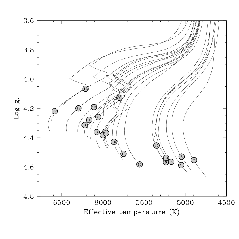
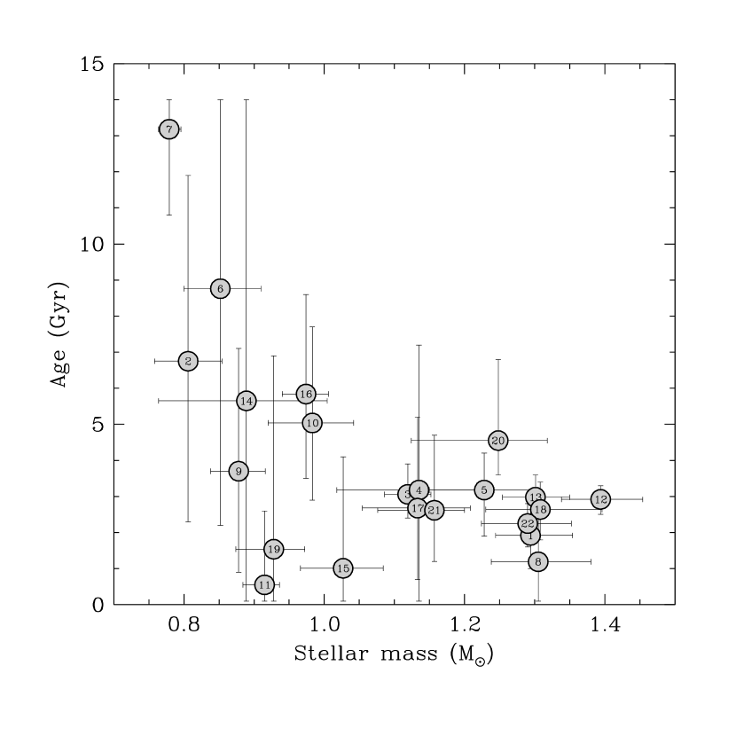
The relative errors of the stellar masses and radii determined here have median values of about 6% and 4%, respectively, but with wide ranges depending on the precision of the observables (2% to 13% for , and 1.3% to 12% for ). While all of the stars in the current sample are hydrogen-burning stars, the degree of evolution within the main sequence varies considerably (see Figure 1). Some systems such as TrES-3 (#11) and XO-1 (#15) are near the zero-age main sequence; others like HAT-P-4 (#20) have already lived for 90% of their main-sequence lifetime. The age is a critical ingredient for the theoretical modeling of the structure and evolution of exoplanets (see, e.g., Burrows et al., 2007), yet it is among the most difficult properties to determine for isolated main-sequence stars. For the host stars of transiting planets the evolutionary ages span the full range, as seen in Figure 2. The difficulty mentioned above is most evident for the less evolved objects ( less than about 0.9 M☉), which are all seen to have large error bars that can reach the upper limit of 14 Gyr considered here. For those cases the nominal ages reported in this work should be used with caution.
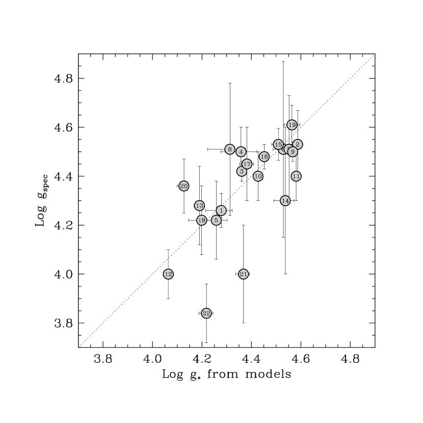
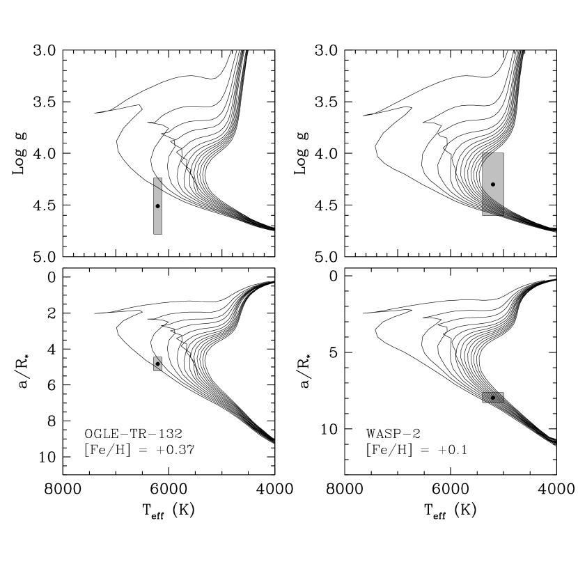
The surface gravities inferred from the models (; Table 3) have formal uncertainties that are typically about 5 times smaller than those measured spectroscopically (; Table 1). This reflects the strength of the constraint provided by . The values of and are compared against each other in Figure 3. On average they agree quite well (the mean difference is dex), and the rms scatter of the differences is 0.15 dex although three of the systems present differences larger than 0.2 dex. An illustration of the superior constraint afforded by is shown in Figure 4 for OGLE-TR-132 and WASP-2, two of the more dramatic examples. In neither case is the parallax known.
3. Comparison with other models
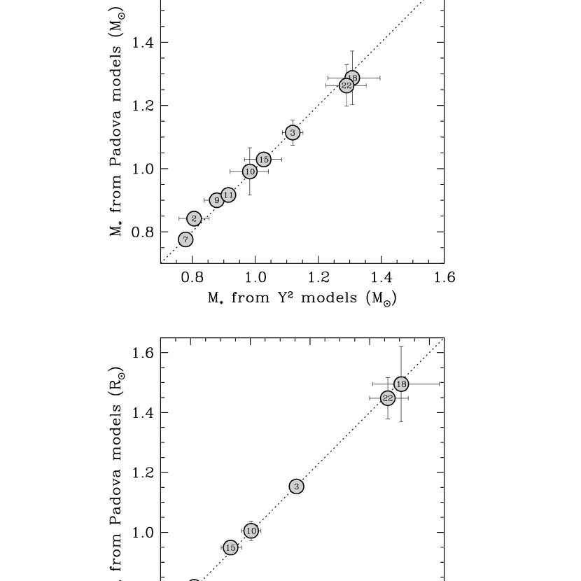
There is undoubtedly some systematic error introduced by imperfections in the stellar evolution models themselves, but this type of error is difficult to evaluate. Extensive comparisons between models and observations using double-lined eclipsing binaries with very accurately measured masses and radii have shown that the agreement with theory is in general very good, and is within a few percent for solar-type stars (see, e.g., Andersen, 1991; Pols et al., 1997; Lastennet & Valls-Gabaud, 2002). As a simple test, we considered a second set of models by Girardi et al. (2000) that has often been used by other investigators in the field of transiting planets. We used the isochrone interpolation tools provided on the web site at the Osservatorio Astronomico di Padova333http://stev.oapd.inaf.it/lgirardi/cgi-bin/cmd. to explore the agreement with the observed values of , [Fe/H], and , and to infer the stellar mass and other properties in the same way as above. There are small differences in the physical assumptions between these models and those from the Y2 series, but overall they are rather similar. For this application the Padova models are available for metallicities smaller than (corresponding to [Fe/H] ), which allows us to compare results for nine of the transiting systems.444Higher-metallicity Padova models have been published by Salasnich et al. (2000), but those employ physical assumptions different enough that they cannot be merged with the Girardi et al. (2000) models we use here. In addition, from a practical point of view, the use of these higher-metallicity models is not yet implemented in the online interpolation routine as of this writing. Figure 5 displays this comparison for the stellar masses and radii, showing that in all cases the results from both models agree to well within their uncertainties.
Similar tests were carried out using the models of Baraffe et al. (1998). These models enjoy widespread use for lower-mass stars and brown dwarfs, but they are also computed for masses as large as 1.4 M☉. They are available for three different values of the mixing length parameter over restricted ranges in mass and metallicity. The value that fits the observed properties of the Sun (against which all models are calibrated) is . For cooler objects near the bottom of the main sequence the value used almost universally is . Here we adopt the former value, since our stars are all more massive than about 0.8 M☉ with the exception of GJ 436, which we discuss in more detail in § 5. For the mass range of interest and for the Baraffe et al. (1998) models are publicly available only for solar metallicity, so the comparison was limited to transiting systems with [Fe/H] within about 0.1 dex of the Sun, and with [Fe/H] uncertainties that keep them within 0.2 dex of solar. Of the six systems in this range, one (OGLE-TR-113) gave no solution consistent with the observed values of and . This is because the Baraffe models are limited to ages less than about 10 Gyr for this mass range, whereas both the Yi et al. (2001) and the Girardi et al. (2000) models indicate an age of about 13 Gyr for this star. Whether OGLE-TR-113 is truly this old is unknown. It seems at least as likely that some of the other observational constraints are in error. The remaining 5 systems show excellent agreement with the results from both the Y2 models and the Padova models, within the formal uncertainties.
These tests of the stellar evolutionary models are obviously not exhaustive, and it may well be the case that all of the sets of models we considered have some deficiencies in common. However, the general pattern of agreement does lend some degree of confidence to the results. We proceed under the assumption that the systematic errors in these calculations are not the dominant source of error in the stellar parameters derived here (except perhaps for OGLE-TR-113, as noted above).
4. Additional observational constraints
As a further test of the accuracy of our stellar radius determinations, in this section we consider the consistency check provided by the near infrared (NIR) surface brightness (SB) relations, which yield the angular diameter of a star directly in terms of its apparent magnitude and color. Unlike the parallax, which would in principle yield the stellar luminosity but is known for only five of the brighter systems in the sample, can be computed for all host stars from existing photometry. We use the empirical relation
| (4) |
derived by Kervella et al. (2004), in which the coefficients are and , the -band magnitude is in the Johnson system, and is the limb-darkened value of the angular diameter expressed in milli-arc seconds. The relation represented by eq. (4) is extremely tight, with a scatter well under 1%. Near infrared magnitudes are available for all stars from the 2MASS catalog and were transformed to the Johnson system following Carpenter (2001). The best available magnitudes collected from the literature are listed in Table 1.
Angular diameters from our stellar evolution modeling in § 2.3 can be derived for comparison with by making use of our theoretical radii and absolute visual magnitudes in Table 3, along with the apparent magnitudes, using
| (5) |
With the stellar radius expressed in solar units, the numerical constant is such that is in mas. Neither this equation nor the previous one take into account interstellar extinction, although eq. (4) is actually quite insensitive to extinction. We discuss this below.
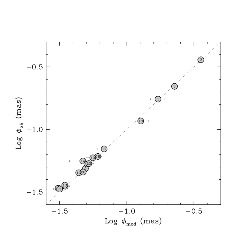
The comparison between the angular diameters from eq. (4) and eq. (5) is shown in Table 4 for all systems except for GJ 436, for reasons to be described in the next section, and the OGLE stars, which are likely to be significantly affected by extinction since they lie several kpc away near the Galactic plane. The uncertainties listed include all contributions from the photometry and model-derived quantities, as well as the errors in the coefficients of eq. (4). The precision of is typically several times better than that of . A graphical comparison is shown in Figure 6, with the one-to-one relation represented with a diagonal line. The good agreement over the full range of an order of magnitude in is an indication that our model radii from § 2.3 are accurate.
One effect of extinction in this analysis would be to make the values based on eq. (5) appear too small. Examination of the differences shows a hint of this, particularly among the fainter (more distant) stars: the average difference is for the 6 objects brighter than , and for the others. Since reddening values for individual systems are presently unknown, and cannot be determined accurately enough from the information at hand, we are unable to correct for this. We are equally unable to turn the argument around and use the values as further constraints in our modeling. By trial and error we find that a uniform reddening value between and 0.03 is sufficient to reduce the average discrepancy in the angular diameters for the fainter stars to zero. This modest amount of reddening is consistent with expectations for objects that are between 100 and 500 pc away, as are these.
In addition to the angular diameters, Table 4 lists the parallaxes and corresponding distances we derive from and , ignoring extinction. Hipparcos parallaxes are given for comparison as well, for the objects that have them.
5. The case of GJ 436
As the only M dwarf among the currently known transiting planet host stars, GJ 436 presents a special challenge. The Y2 stellar evolution models we used in all other cases are not intended for the lower main sequence, as they lack the proper non-grey model atmosphere boundary conditions to the interior equations that have been shown to be critical for cool objects (see, e.g., Chabrier & Baraffe, 1997). The Padova models of Girardi et al. (2000) have the same shortcoming, although both of these models are perfectly adequate for hotter stars. On the other hand, the calculations by Baraffe et al. (1998) with are specifically designed for low-mass stars, and have in fact been invoked by other authors for this system as a rough consistency check. For the most part, the previous mass determinations for GJ 436 have relied upon empirical mass-luminosity relations, but even those relations have their problems. Previous radius estimates for GJ 436 have often rested on the assumption of numerical equality between and for M stars (Gillon et al., 2007a; Deming et al., 2007).
The importance of the GJ 436 system is undeniable, as it harbors the smallest transiting planet that has been found to date (comparable in size to Neptune). Furthermore, it is the nearest transiting exoplanet, at a distance of only 10 pc. Given these facts, it is somewhat surprising that until recently the mass of the star (0.4 M☉) was only known to about 10% (Maness et al., 2007; Gillon et al., 2007b), on a par with the worst of the determinations in Table 3 (that of WASP-2, with poorly determined spectroscopic parameters and more than 10 times farther away). Similar limitations hold for the stellar radius. As a result, our knowledge of the planetary parameters has suffered. Torres (2007) showed that the Baraffe et al. (1998) models in their original form do not yield satisfactory results for GJ 436 since different answers for and are obtained depending on which constraints are used (including the absolute magnitude, since a reliable parallax measurement is available from Hipparcos). Moreover, some of the other predicted quantities are at odds with empirical determinations. These difficulties had not been previously emphasized.
However, as described by Torres (2007), reliable parameters can still be obtained from the models by modifying the theoretical radii and temperatures in such a way as to preserve the bolometric luminosities. This recognizes the fact that and as predicted by theory have been shown to disagree with accurate measurements for M dwarfs in double-lined eclipsing binaries (see, e.g., Popper, 1997; Clausen et al., 1999; Torres & Ribas, 2002; Ribas, 2003; López-Morales & Ribas, 2005), whereas the luminosities appear to be unaffected (Delfosse et al., 2000; Torres & Ribas, 2002; Ribas, 2006; Torres et al., 2006). Torres (2007) applied simultaneously the observational constraints on , , the color index , and the absolute -band magnitude , and allowed the radius/temperature adjustment factor to be a free parameter. In this way a self-consistent solution was achieved for all parameters, and in addition the radius/temperature factor showed excellent agreement with previous estimates for other M dwarfs. The stellar mass and radius are M☉ and R☉. We adopt these results here, thus placing GJ 436 on a similar footing as the other transiting systems in that the properties of the host stars are all based on current stellar evolution models.
The results for GJ 436 are listed in Table 3 along with those of the other 22 stars. A few words of caution are in order. As pointed out by Torres (2007), the predicted absolute visual magnitude for this star is unreliable due to missing molecular opacity sources shortward of 1 m in the model atmospheres that are used as boundary conditions in the stellar evolution calculations (see, e.g., Baraffe et al., 1998; Delfosse et al., 2000). Also, because of the unevolved status of the star, the nominal age is probably meaningless since the observational constraints allow any age within the range of 1–10 Gyr explored in the modeling effort of Torres (2007). Finally, this modeling effort assumed that the stellar metallicity is solar. For GJ 436 this is a valid assumption since the measured composition is [Fe/H] (see Appendix), but the uncertainty in [Fe/H] was not accounted for due to the lack of proper models, and therefore the errors of the stellar properties in Table 3 may be underestimated.
A careful reader may wonder whether our use of the Baraffe et al. (1998) models in § 3 as a check on the results from the Y2 isochrones is contradicted by our remarks on the radius/temperature discrepancies mentioned above. We do not believe so, because the mass regime of GJ 436 is very different. The host stars of the other transiting planets are typically more than twice as massive as GJ 436.
6. Planetary parameters
The combination of the stellar properties in Table 1 with the light curve parameters in Table 2, along with the measured orbital periods and velocity semi-amplitudes, yields the homogeneous set of planet parameters presented in Table 5. In addition to the planetary mass and radius, we have computed and tabulated the planetary surface gravity and mean density, as well as the orbital semimajor axis and other useful characteristics. As pointed out by Southworth et al. (2007), Winn et al. (2007), Beatty et al. (2007), and others, the surface gravity of a transiting planet can be derived without knowledge of the stellar mass or radius, using only the radial-velocity curve and the transit light curve. We take this opportunity to correct the general expression for presented by Sozzetti et al. (2007), valid also for the case of eccentric orbits, which neglected to account for the projection factor implicit in the impact parameter as derived from the light-curve fits:
The numerical constant is such that the gravity is in cgs units when and are expressed in their customary units of days and m s-1.
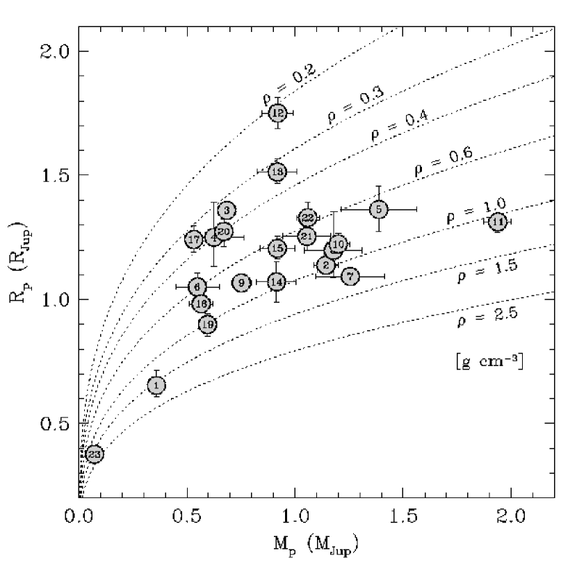
The first properties one generally wants to know about a transiting planet are its mass and radius. The large size measured for the first transiting planet discovered, HD 209458b, has been widely debated and still presents somewhat of a challenge to theory. It is now accompanied by several other inflated planets, underlying our incomplete knowledge of the physics of these objects. An updated version of the now classical diagram of versus is shown in Figure 7, in which five other examples are seen to be at least as large as HD 209458b (#3), or perhaps even larger, given the uncertainties.
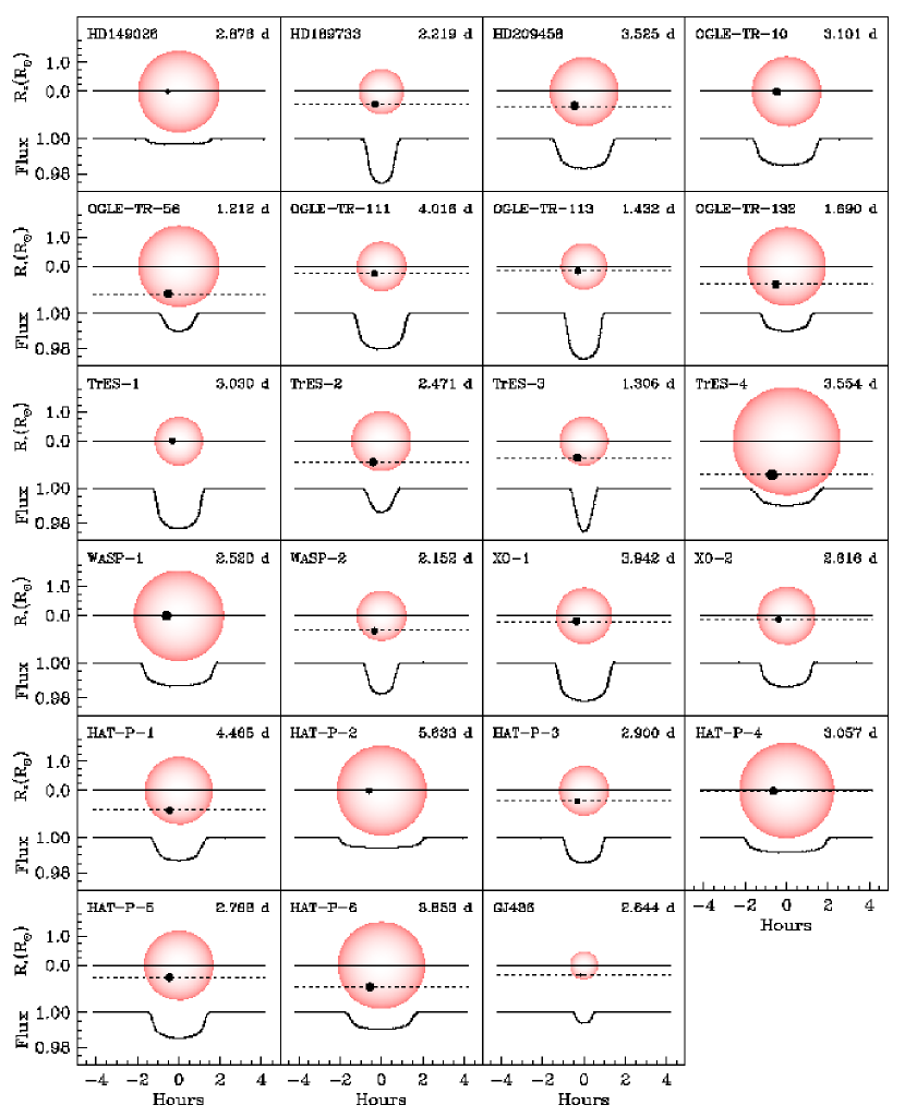
The fundamental physical properties of the known transiting planets cover a considerable range—more than two orders of magnitude in mass, a factor of nearly 5 in radius, and a factor of 3 in orbital separation—and these are discussed in the next section. But the geometric properties that determine the light-curve shapes are also varied. In Figure 8 we present a “portrait gallery” of all known transiting planets. Stars and planets are rendered to scale, emphasizing the wide range of stellar types probed by the photometric searches. The orbital geometries are indicated with solid horizontal lines representing an edge-on orientation, and the path of each planet across the stellar disk shown with dotted lines at the actual impact parameter. (Of course, the data do not distinguish between positive and negative impact parameters.) The resulting light curves calculated for the band are all shown with the same vertical (flux) and horizontal (time) scale, to facilitate comparison. Depths vary quite significantly (3 mmag in for HD 149026b, 26 mmag for OGLE-TR-113b; see Table 2), as do the overall shapes of the transit events, which in several cases are grazing enough to depart from the canonical profiles often depicted in the literature.
7. Discussion
Many investigators have sought and claimed possible correlations between various stellar and planetary parameters of transiting systems. In principle such correlations could lead to important insights into the formation, structure, and evolution of exoplanets. A primary motivation for presenting a more complete, accurate, and homogeneous set of these parameters in this work was to facilitate such studies. The relatively large array of properties now available offers the opportunity to find new correlations, or to revisit old ones incorporating additional variables. While it is beyond the scope of the present work to investigate all possible correlations with statistical rigor, in this section we check on three of the most intriguing and potentially important relations that have been proposed.
7.1. Planetary mass versus orbital period
Mazeh et al. (2005) were the first to point out the apparent correlation between and for transiting planets (see also Gaudi et al., 2005). The original suggestion was based on only 6 systems, but additional discoveries have generally supported the trend of decreasing mass with longer periods, although the scatter has also become larger. This is shown in Figure 9a. HAT-P-2b would be an extreme outlier in this plot; we have excluded it because it is so much more massive than the other planets and may belong to a different category of planet (see § 7.2). Similarly, we have excluded GJ 436b because it is so much less massive than the others, and may be a rocky or rock-ice planet rather than a gas giant. A simple linear fit is shown for reference (dashed line).
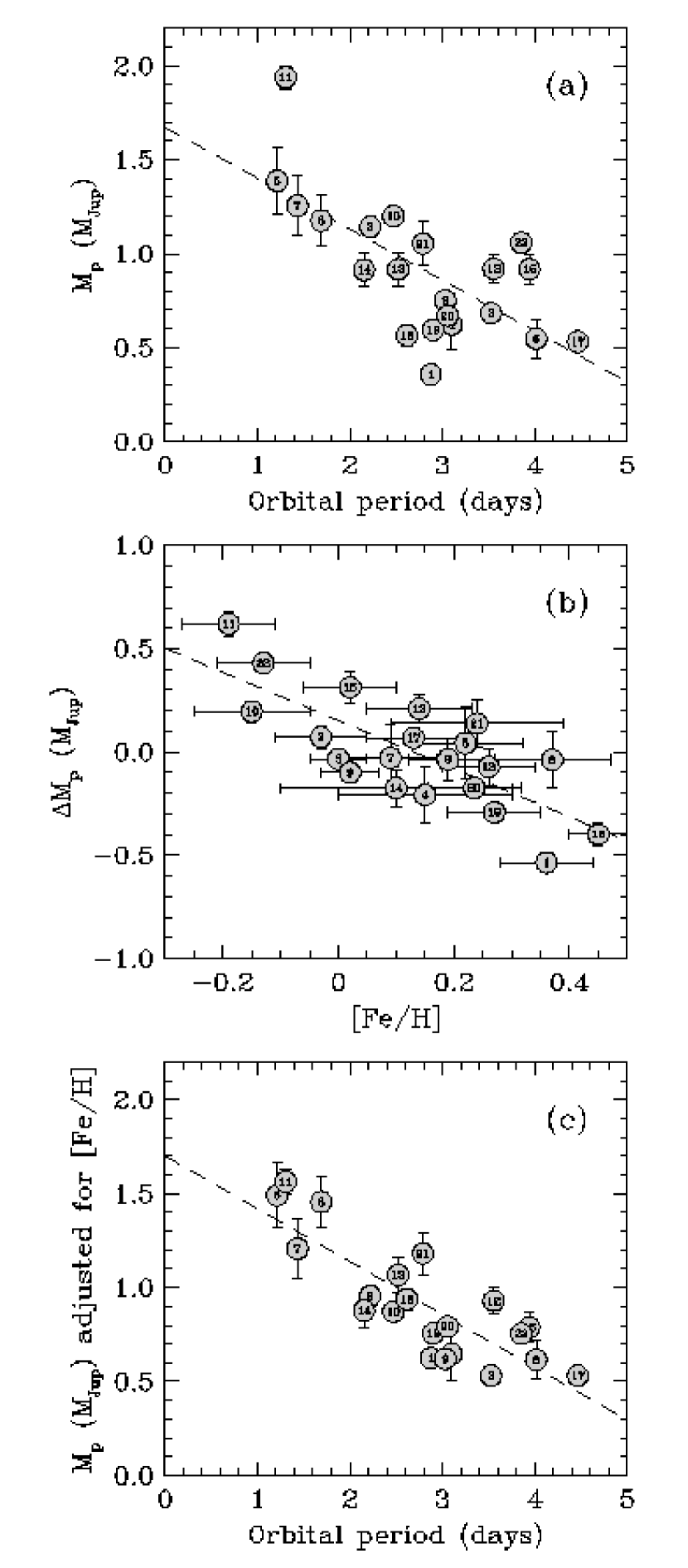
We also investigated the scatter in this relation, seeking any “third variable” that might correlate with the residuals. We seem to have found such a third variable: the metallicity of the host star. Figure 9b displays the residuals from the top panel as a function of [Fe/H], indicating a rather clear correlation (dashed line): . After removal of this trend, the relation between and period becomes tighter (Figure 9c). The scatter in the mass-period relation is reduced from 0.26 MJup in the top panel to 0.17 MJup in the bottom panel. It seems unlikely that this is a statistical fluke. However, the scatter is still larger than the formal observational uncertainties, suggesting that these three variables are not completely determinative.
What might be the implications of this metallicity dependence? It has been proposed that the mass-period relation is related to the process by which close-in exoplanets migrated inward from their formation sites, or more specifically, to the mechanism that halts migration at orbital periods of a few days. The trend of larger masses at shorter orbital periods could suggest that the halting mechanism depends on mass, and larger planets are able to migrate further in. The dependence on metallicity may then be interpreted to indicate that planets in metal-poor systems need to be more massive in order to migrate inward to the same orbital period as more metal-rich planets. In this context, the trend in Figure 9b could be interpreted as evidence that the efficiency of the migration (or halting) mechanism is affected to some degree by the chemical composition. A dependence of migration on metallicity is in fact predicted by some theories, and could arise, as pointed out by Sozzetti et al. (2006), either from slower migration rates in metal-poor protoplanetary disks (Livio & Pringle, 2003; Boss, 2005) or through longer timescales for giant planet formation around metal-poor stars, which would effectively reduce the efficiency of migration before the disk dissipates (Ida & Lin, 2004; Alibert et al., 2005). However, the above processes are more aimed at addressing the apparent lack of short-period planets among very metal-poor stars claimed by some authors (see Sozzetti et al., 2006), whereas among the transiting planets it is not the lack of more metal-poor examples we are concerned with, but rather their different properties (such as mass) compared to metal-rich planets at the same orbital period. To give a quantitative example, we find that for a period of 2.5 days (near the average for known transiting systems), the mass of a planet with [Fe/H] is 40% larger than one with average metallicity ([Fe/H] = +0.13, excluding HAT-P-2b and GJ 436b), while the mass of a planet with [Fe/H] is about 30% smaller. This range of metallicities, from [Fe/H] to +0.4 (covering a factor of 4 in metal enhancement), is approximately the full range observed. We note that the strength of the metallicity effect is modest rather than overwhelming, and this too is in agreement with theoretical expectations (e.g., Livio & Pringle, 2003). The massive planet HAT-P-2b obviously does not conform to this trend of versus period, which may indicate some fundamental difference either in its formation or migration.
An alternative interpretation, also proposed by Mazeh et al. (2005), is that the versus relation is more a reflection of survival requirements in close proximity to the star, due to thermal evaporation from the extreme UV flux. Close-in planets must be more massive to avoid ablation to the point of undetectability. The role of metallicity in this case would be through the difference in the internal structure (Santos et al., 2006). Metal-rich planets have been suggested to be more likely to develop rocky cores (Pollack et al., 1996; Guillot et al., 2006; Burrows et al., 2007, see also § 7.3). If the presence of such a core somehow slows down or prevents complete evaporation, as has been proposed (Baraffe et al., 2004; Lecavelier des Etangs et al., 2004), survival at a given period would then have a dependence on metallicity.
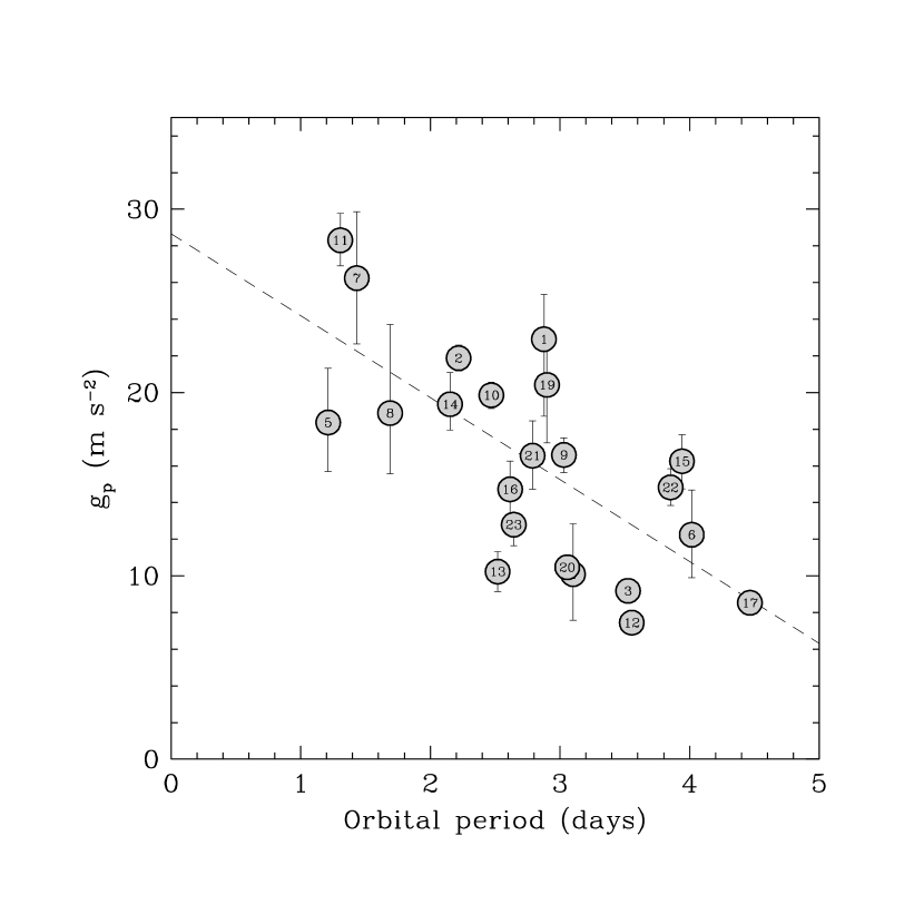
A diagram related to the one considered above is that of planetary surface gravity versus orbital period, first presented by Southworth et al. (2007). Because does not require knowledge of the mass or radius of the star, it is in a sense a cleaner quantity that should be free from systematic errors in and and is nearly independent of stellar evolution models. This not true of other bulk properties such as the mean planet density. An updated version of the versus relation is shown in Figure 10, along with a linear fit. We examined the residuals from this linear fit for a possible correlation with stellar metallicity, as we did earlier for the case of the versus diagram, but we found none. Given that , we note that the apparent influence of metallicity on the planetary radii must be contributing significantly to the scatter in the versus period relation. We discuss this further in § 7.3.
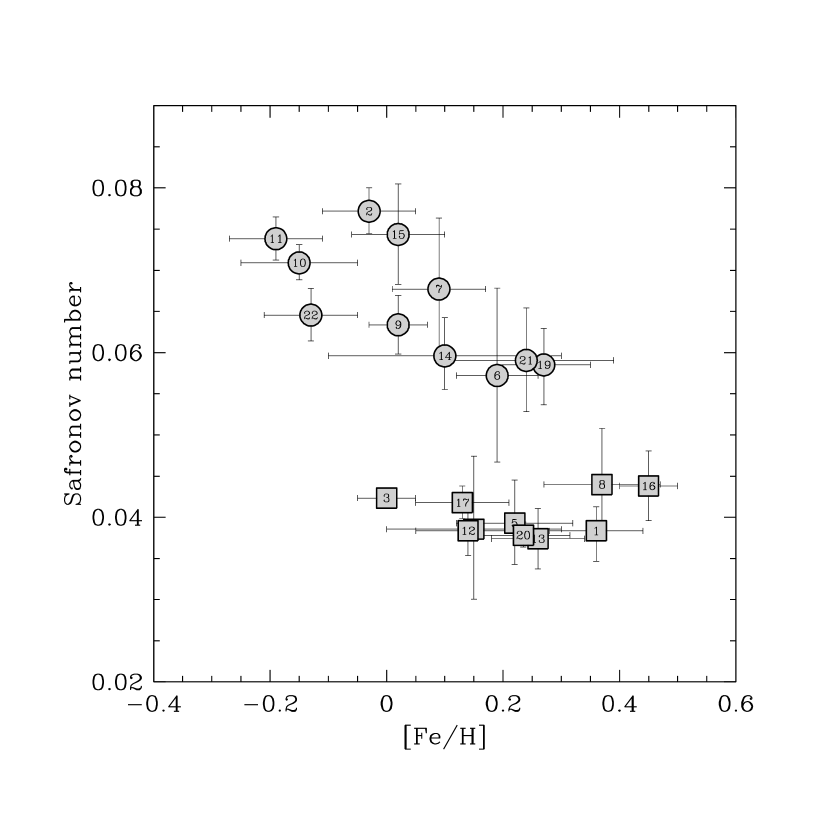
7.2. Safronov number versus equilibrium temperature
Recently, Hansen & Barman (2007) proposed a distinction between two classes of hot Jupiters, based on a consideration of the Safronov number and the zero-albedo equilibrium temperature. The Safronov number is a measure of the ability of a planet to gravitationally scatter other bodies (Safronov, 1972), and is defined as , the ratio between the escape velocity and the orbital velocity squared. We assume that the zero-albedo equilibrium temperature scales as (i.e., we assume that the heat redistribution factor is common to all planets, in the absence of more complete knowledge).
We list and for all transiting planets in Table 5. Hansen & Barman (2007) pointed out a gap in the distribution of Safronov numbers, and defined Class I planets as those with and Class II as . They tentatively proposed also that these two categories have other distinguishing characteristics, such as a difference in the average temperature of the host stars, or the orbital separations. Upon the discovery of HAT-P-5b (Bakos et al., 2007c) and HAT-P-6b (Noyes et al., 2007), those authors pointed out that the distinction now seems less clear, as these two planets tend to fill the gap between Class I and Class II.
The larger sample now available, and especially the more accurate and homogeneous set of properties presented here, offers the opportunity to revisit the issue. Figure 11 shows an updated version of the – diagram for transiting planets, which has some significant differences compared to the original version. Following Hansen & Barman (2007) we have excluded the massive planet HAT-P-2b, with a Safronov number so much larger than all the others () that it would seem to be in a different class altogether, as well as GJ 436b, which is of much lower mass and a presumably different composition.
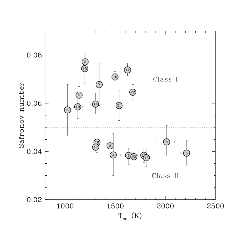
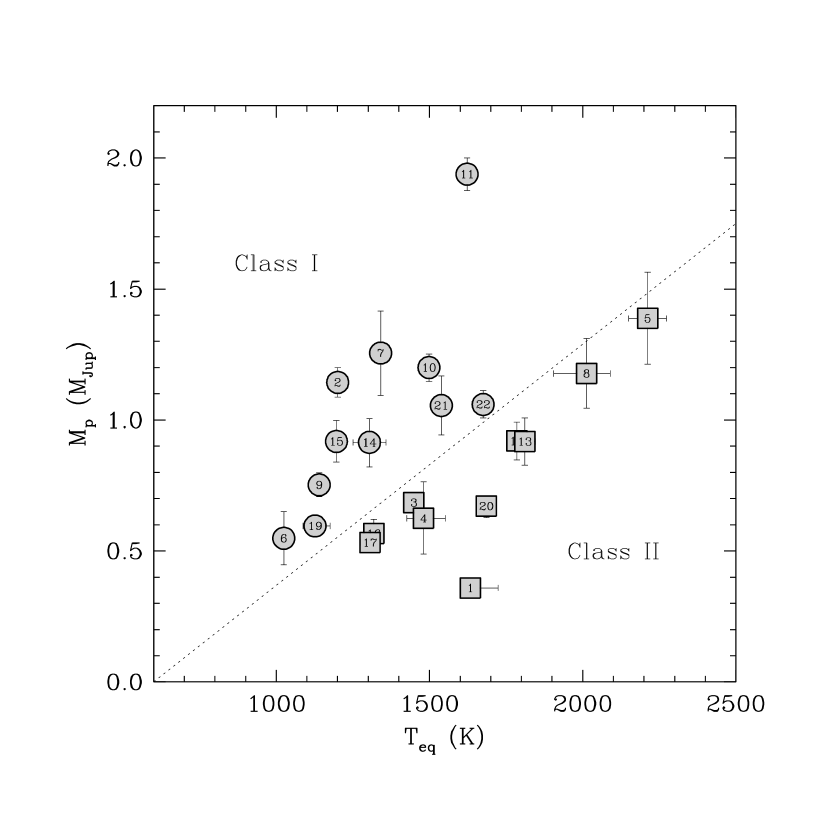
In our updated diagram the separation between Class I and Class II is still quite striking. The clustering of the Class II objects around the value has tightened, if anything, and HAT-P-5b (#21) and HAT-P-6b (#22) do not encroach on the gap in Safronov numbers with Class I. (The Class II object with the lowest value of is OGLE-TR-111b [#6].) Thus, the dichotomy remains very suggestive. Hansen & Barman (2007) have argued that the principal distinction between the two classes is based on mass (planetary and/or stellar), and that planets of Class II are, on average, less massive than those in Class I, and orbit stars that are typically more massive. While we agree with the latter part of this statement regarding the stellar masses, we find that the distribution of planetary masses is indistinguishable between the two groups. We do confirm, however, that an updated diagram of versus (see Figure 12) shows planets in Class II to be systematically less massive for the same equilibrium temperature (level of irradiation), as was also found by Hansen & Barman (2007), so in this sense their general claim that the distinction has something to do with mass seems to be supported by the observations.
An important characteristic that seems to be different in the two groups is the metallicity of the parent stars. This is illustrated in Figure 13. Parent stars of Class II planets tend to be slightly more metal-rich. A Kolmogorov-Smirnov test of the two metallicity distributions, which appear to be centered around [Fe/H] for Class I and [Fe/H] for Class II, indicates only a 1.7% probability that they are drawn from the same parent population. There is perhaps a hint that the Safronov numbers for Class I planets show a decreasing trend with metallicity in Figure 13, whereas the values for Class II planets are independent of [Fe/H].
7.3. Heavy element content versus stellar metallicity
Transiting planet discoveries have challenged our theoretical understanding of these objects from the very beginning. The inflated radius of HD 209458b, argued to be due to an overlooked internal heat source in the planet (see, e.g., Fabrycky et al., 2007, and references therein), still poses a problem for modelers, and this first example is now joined by several other oversized planets indicating it is not an exception (see § 6). On the other end of the scale, HD 149026b was the first transiting giant planet found to have a radius significantly smaller than predicted by standard theories (Sato et al., 2005). The implication is that it must have a substantial fraction of heavy elements of perhaps 70 M⊕ (2/3 of its total mass), which is often assumed to be in a core. More recently HAT-P-3b (Torres et al., 2007) has also been found to be enhanced in heavy elements on the basis of its small size for the measured planet mass. In this case metals make up 1/3 of the total mass.
Guillot et al. (2006) and also Burrows et al. (2007) have found evidence that the heavy element content correlates with the metallicity of the parent star, a trend that was not anticipated by theory. These studies were based, respectively, on the 9 and 14 transiting planets known at the time. The larger sample now available warrants a second look at this possible correlation, for its potential importance for our understanding of planet formation.
Here we have estimated the heavy element content of each planet using the recent models by Fortney et al. (2007), which include the effects of irradiation from the central star. The mass in heavy elements was calculated from the measured mass of the planet, its radius, the orbital semimajor axis, and the age of the system as derived above from stellar evolution models. The uncertainty in these estimates is often very large, due mostly to errors in the measured values of and especially the age. In ten cases the models indicate no metal enhancement at all, and some of these are in fact “inflated” hot Jupiters. In a few other cases only an upper limit can be placed. For HAT-P-2b the Fortney et al. (2007) models as published do not provide a large enough range of core masses. The results for are listed in Table 5. A comparison with values from Guillot et al. (2006) and Burrows et al. (2007) for the subset of planets in common indicates significant differences in some cases, either in or its error.
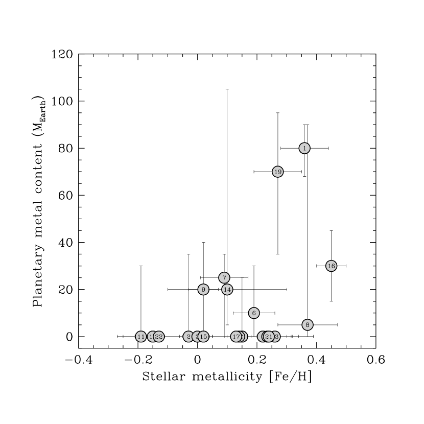
The mass in heavy elements is plotted against the stellar metallicity in Figure 14. The overall trend is similar to that pointed out by previous authors, in the sense that the upper envelope of the distribution appears to increase with [Fe/H]. It is natural to expect that a higher stellar metallicity implies a higher-metallicity protoplanetary disk. In the context of the core-accretion model of planet formation, one would also naturally expect a more metal-rich disk to lead to more metal-rich planets, and in this sense the observed trend is in accordance with the core-accretion theory.
8. Final remarks
Progress in understanding planet formation, structure, and evolution depends to a large extent on an accurate knowledge of their physical characteristics. This begins with an accurate knowledge of the properties of the parent stars. The main contributions of this work toward that goal are a re-analysis of all available transit light curves with the same methodology and the uniform application of the best possible observational constraints to infer the stellar mass and radius. This includes, in particular, the constraint on the stellar density through the light-curve parameter . We expect the application of this technique to current and future ground-based or space-based transit searches to be highly beneficial, especially when parallax information for the candidates is unavailable.
Through the procedures described above we have obtained a more homogeneous set of stellar and planetary parameters than previously available, with error bars that are well understood and more appropriate when searching for patterns and correlations among the various quantities. The results have enabled us to explore the role of metallicity in two of the more intriguing correlations between star and planet properties: that of versus , to which Mazeh et al. (2005) first drew attention, and that of the Safronov number versus equilibrium temperature (Hansen & Barman, 2007). We have also re-examined the correlation between the stellar metallicity and the heavy-element content of the planets. We find a clear influence of [Fe/H] in the versus diagram, with the planets in more metal-poor systems being systematically more massive at a given orbital period. This can be interpreted as evidence of a (mass and) metallicity dependence of the migration process. Alternatively it may be seen as indirect support for the correlation between core size and [Fe/H] along with the idea that the presence of such cores slows down or prevents complete evaporation of the planets in the extreme radiation environments of these hot Jupiters. We find also that the improved parameters for the present sample of transiting planets support the recently proposed notion of at least two distinct classes of hot Jupiters in terms of their Safronov numbers (Hansen & Barman, 2007). Additionally, the average metallicity of Class II planets appears to be 0.2 dex higher than Class I. Thus, chemical composition adds another distinguishing characteristic to those proposed earlier. A further result of our work, which takes advantage of the larger sample of transiting planets now available, is the confirmation of the general trend of higher heavy-element content for planets with more metal-rich host stars, originally advanced by Guillot et al. (2006) and Burrows et al. (2007).
We expect that the search for other significant correlations will be made easier by the better accuracy and homogeneous character of the properties of the present sample of transiting planets, and should lead to a deeper understanding of their nature.
Appendix A Spectroscopic and photometric information from the literature
Below we describe in detail our compilation of the information available in the literature for the atmospheric parameters of all known transiting planets, as well as the sources for the light curves we have used, and for the velocity semi-amplitudes that determine the planet masses. For the atmospheric parameters (, [Fe/H], ) we consider only spectroscopic studies, and disregard photometric determinations with few exceptions. The values adopted, which are listed in Table 1, are the result of a careful combination of results for each planet rather than the selection of a particular favorite study, and we have therefore deemed it important to document our choices for future reference. For the spectroscopic parameters the goal of this effort has been to arrive at values that best represent the stellar properties based on current knowledge. Combined with our application of uniform procedures for deriving the stellar mass and radius based on state-of-the-art stellar evolution models, we hope that the overall accuracy of the planet parameters has been improved.
1. HD 149026: Two consistent determinations of the effective temperature are available for this star. One is from Masana et al. (2006), who apply a semi-empirical method based on a spectral energy distribution fit (SEDF) calibrated against solar analogs, and the other is from a spectral synthesis analysis by Sato et al. (2005) carried out on high-resolution Subaru spectra using the SME package (Spectroscopy Made Easy, Valenti & Piskunov, 1996; Valenti & Fischer, 2005). We adopt the weighted average of the two, with a generous uncertainty of 50 K. The iron abundance is adopted from Sato et al. (2005), but with a more conservative error of 0.08 dex. The surface gravity is taken from the same source. The velocity semi-amplitude is adopted from Butler et al. (2006). We consider that study, based on 16 RV measurements with the Keck telescope, to supersede the one by Sato et al. (2005), which used fewer Keck velocities (6) combined with 4 velocities with the Subaru telescope, but obtained essentially the same result. Additional Keck velocity measurements (many obtained during transit) were reported recently by Wolf et al. (2007), who also re-reduced the earlier Keck observations of Butler et al. (2006) (for a total of 35). Their study focused on the Rossiter-McLaughlin effect, and did not present a value for . The photometric data used here are the three Stömgren light curves presented by Sato et al. (2005), the Sloan and light curves presented by Charbonneau et al. (2006), and the five light curves presented by Winn et al. (2007e).
2. HD 189733: For we adopt the weighted average of the results by Bouchy et al. (2005a) based on high-resolution CORALIE spectra, and Masana et al. (2006), with an uncertainty of 50 K. Later papers by the first team quote values for (as well as and [Fe/H]) said to be taken from Bouchy et al. (2005a), but which are not exactly the same for reasons that are unclear. We adopt from the Bouchy work, as well as the metallicity, but with an increased [Fe/H] error of 0.08 dex. A study by Gray et al. (2003) based on lower resolution spectra (1.8 Å) gave a somewhat lower temperature (4939 K) along with a much lower value for [Fe/H] of ; we do not consider those results here. The only published determination of is by Bouchy et al. (2005a), which we adopt. Additional RV measurements at Keck were obtained by Winn et al. (2006), mostly during transit for the purpose of studying the Rossiter-McLaughlin effect, but no value of was reported. Ground-based light curves have been obtained in a variety of passbands since the discovery (Strömgren , , , Sloan ). High-quality observations with HST in a passband with an effective wavelength similar to the band were reported by Pont et al. (2007b). These optical observations all suffer to some degree from the fact that the star is relatively active. Spottedness causes irregularities in the photometry, which is very useful to establish the rotational period of the star (see Winn et al., 2007b; Henry & Winn, 2007), but interferes with the accurate determination of the light-curve parameters. By contrast, Knutson et al. (2007) obtained photometry with the Spitzer Space Telescope at the much longer wavelength of 8 m, where spots have a negligible effect. Limb-darkening is virtually non-existent at this wavelength as well, removing another complication. While the ground-based, HST, and Spitzer light curve solutions all agree very well within their uncertainties, for the reasons just described we have chosen in this case to rely only on the Spitzer data, which we have re-analyzed using the same methodology applied to all the other transiting planets. A very similar (but less precise) radius ratio was reported recently by Ehrenreich et al. (2007) based on additional Spitzer observations at 3.6 and 5.8 m.
3. HD 209458: Ten independent determinations of are available, which show excellent agreement: eight are from spectroscopic studies (Mazeh et al., 2000; Gonzalez et al., 2001; Mashonkina & Gehren, 2001; Sadakane et al., 2002; Heiter & Luck, 2003; Santos et al., 2004; Valenti & Fischer, 2005), and two others are based on photometry use the IRFM (Ramírez & Meléndez, 2004) and SEDF (Masana et al., 2006). We adopt the weighted average, with a conservative uncertainty of 50 K. Similarly, we adopt the weighted average of the nine [Fe/H] determinations from the spectroscopic sources, with an error of 0.05 dex. The value we use here is also the weighted average of the eight available measurements. Four values for the semi-amplitude have been published. The early determinations by Mazeh et al. (2000) and Henry et al. (2000) were superseded by more recent studies based on many more RVs and refined analysis techniques by Naef et al. (2004) (46 ELODIE and 141 CORALIE measurements over 5 years, not all published) and Butler et al. (2006) (64 Keck measurements over 6 years). We adopt the weighted average of the results from the two new sources. Our light curve fits are based on the HST/STIS photometry of Brown et al. (2001). In this case, given the high signal-to-noise ratio of the data, we fitted for the quadratic limb-darkening coefficients along with all of the other parameters.
4. OGLE-TR-10: A spectroscopic study by Santos et al. (2006) used 4 co-added UVES spectra to derive , [Fe/H], and . An earlier study by Bouchy et al. (2005b) used a subset of these spectra and somewhat different analysis techniques, and obtained a significantly hotter temperature and a higher metallicity. They also reported an unusually large surface gravity for the temperature they obtained (, for K). Because these results may be affected by the strong correlations often present between all these quantities, we have preferred not to use the Bouchy et al. (2005b) values here. Another recent study by Holman et al. (2007a) supersedes previous analyses by Konacki et al. (2003a) and Konacki et al. (2005) based on similar material, which, nevertheless gave essentially the same results with only slightly different errors. The Santos and Holman values for ( K and K, respectively) are somewhat discrepant (by 275 K, or 2.1). We note that the direction of the difference is consistent with the sign of the difference in the iron abundances of these two studies (Santos giving , and Holman ), given the typical correlation between these two quantities. Both teams have presented evidence supporting their determinations (a good fit to the H line profile in the case of Santos et al., and agreement with the H profile as well as a consistency check using line-depth ratios, for Holman et al.). Under these circumstances we simply adopt intermediate values (arithmetic averages) for , [Fe/H], and , with increased uncertainties of 130 K, 0.15 dex, and 0.10 dex, respectively. Two consistent determinations of have been reported: one by Bouchy et al. (2005b) based on 14 RVs from UVES/FLAMES, and the other by Konacki et al. (2005). We adopt the latter results, because they are based on a combination of 9 Keck measurements with the 14 RVs from Bouchy et al. (2005b). The light-curve parameters are taken from the work of Pont et al. (2007a), who combine the best photometry available.
5. OGLE-TR-56: The adopted temperature, metallicity, and surface gravity for this star are the weighted averages of three fairly consistent spectroscopic determinations (Konacki et al., 2003b; Bouchy et al., 2005b; Santos et al., 2006). Conservative errors of 100 K, 0.10 dex, and 0.16 dex are assigned to those quantities, respectively. Two determinations of the semi-amplitude are considered here: one by Torres et al. (2004), who used 11 Keck RVs and whose study supersedes Konacki et al. (2003b), and one by Bouchy et al. (2005b), based on 8 UVES and 5 HARPS measurements. We adopt the weighted average of the two results. Our light curve fits are based on the and data of Pont et al. (2007a).
6. OGLE-TR-111: The atmospheric parameters for this system are adopted from the spectroscopic study by Santos et al. (2006), based on 6 UVES spectra, which supersedes those in the discovery paper by Pont et al. (2004) that used only a subset of the same spectra. The errors seem realistic, so we adopt those as well. The only determination of available is from Pont et al. (2004). Our photometric solutions are based on the two -band light curves of Winn et al. (2007f).
7. OGLE-TR-113: Three spectroscopic determinations of , [Fe/H], and give very consistent results (Bouchy et al., 2004; Konacki et al., 2004; Santos et al., 2006), and we adopt the weighted average. The formal uncertainties are very small because of the (likely accidental) good agreement; to be conservative we have increased them to 75 K, 0.08 dex, and 0.22 dex, respectively. For we have taken the weighted average from the first two sources above, which are based, respectively, on 8 spectra from UVES and 7 from Keck. Our light curve fits use the band photometry of Gillon et al. (2006).
8. OGLE-TR-132: The temperature, metallicity, and surface gravity are taken from Gillon et al. (2007a). This high-resolution study, based on UVES spectra, supersedes an earlier one by Bouchy et al. (2004), which had very large uncertainties. The velocity semi-amplitude is adopted from the work of Moutou et al. (2004), who obtained a value some 20% larger than in the discovery paper of Bouchy et al. (2004) despite having used the same 5 original RV measurements. The difference is due solely to the improved ephemeris provided by Moutou et al. (2004) based on a new, high-quality light curve gathered with the VLT, compared to the original ephemeris from the OGLE photometry. Our light curve fits use the VLT -band photometry of Gillon et al. (2007a).
9. TrES-1: Four high-resolution spectroscopic analyses of this star giving consistent results have been published by Alonso et al. (2004), Sozzetti et al. (2004), Laughlin et al. (2005), and Santos et al. (2006). We adopt the weighted averages of those studies. The metallicity from Alonso et al. (2004) was assigned here an uncertainty (not originally reported) of 0.2 dex based on previous experience with the same type of material. As before, we have chosen more conservative errors of 50 K for and 0.05 dex for [Fe/H], to account in the latter case for the fact that Santos et al. (2006) find a hint of small systematic differences with Sozzetti et al. (2004). The mean metallicity is close to solar: [Fe/H] . A claim has been made by Strassmeier & Rice (2004) of a much lower metallicity for TrES-1 of [Fe/H] (no error given). This is so discrepant compared to other four determinations that it is most likely incorrect. For , the only value appearing in the literature is that of Alonso et al. (2004), based on 8 Keck spectra, which we adopt. Laughlin et al. (2005) made 5 additional RV measurements, also with Keck, and combined them with the Alonso velocities to improve the planet mass. However, no value for was reported and it is not possible to recover it accurately from other published quantities. Our light curve fits use the Sloan -band photometry of Winn et al. (2007d).
10. TrES-2: A single source is available for the atmospheric parameters (Sozzetti et al., 2007), and those values are adopted here. Although the published uncertainty in is only 50 K, a number of checks on the temperature are presented that suggest the value is accurate, and thus we accept that error. The semi-amplitude is adopted from the discovery paper by O’Donovan et al. (2006). Our photometric solutions rely on the -band light curves of Holman et al. (2007b).
11. TrES-3: The atmospheric properties were taken from Sozzetti et al. (in preparation), while the semi-amplitude and the light-curve parameters are adopted from the discovery paper by O’Donovan et al. (2007).
12. TrES-4: The atmospheric properties were taken from Sozzetti et al. (in preparation), while the semi-amplitude and the light-curve parameters are adopted from the discovery paper by Mandushev et al. (2007).
13. WASP-1: The spectroscopic investigation by Stempels et al. (2007) based on NOT/FIES spectra supersedes the results in the discovery paper by Collier Cameron et al. (2007), and in fact the new study claims that the SOPHIE spectra in the old one were compromised by scattered light and uncertain normalization. Despite this, the results for the atmospheric quantities are quite similar. We adopt the parameters from the new study, although with more conservative uncertainties of 75 K, 0.08 dex, and 0.16 dex for , [Fe/H], and . The only RV analysis available is that by Collier Cameron et al. (2007), based on 7 RV measurements with SOPHIE. Our light curve fits are based on the -band photometry of Charbonneau et al. (2007).
14. WASP-2: For this system there are no spectroscopic studies beyond the one in the discovery paper by Collier Cameron et al. (2007), in which the uncertainties for and are rather large. Nevertheless, the temperature appears to be accurate as shown by a consistency check obtained using the IRFM. The authors state that the abundances are not substantially different from solar, and they appear to adopt, according to the caption of their Table 3, a value of [Fe/H] . This may simply be a representative abundance, but it is a reasonable value since it is close to the average metallicity of the other transiting planets. We accept it for lack of a better determination, along with and as reported. We take also the value from this paper, which is based on 9 RV measurements with SOPHIE. Our light curve fits use the -band photometry of Charbonneau et al. (2007).
15. XO-1: The discovery paper by McCullough et al. (2006) presents the only spectroscopic study of this system. The atmospheric parameters are based on HJS spectra from the 2.7m telescope at McDonald Observatory, analyzed with SME. We adopt the temperature and metallicity from this source, with increased uncertainties of 75 K and 0.08 dex. The value is adopted also as given there. The semi-amplitude derived by these authors is based on 10 RV measurements from HET and the 2.7m (HJS). Our light curve fits are based on the -band photometry of Holman et al. (2006).
16. XO-2: The values of , [Fe/H], and derived in the discovery paper by Burke et al. (2007) are adopted here as published, and are based on two spectra collected with the HET for this northern component of a 31″ visual binary. The logarithmic iron abundance, , is found to be very similar to that obtained for the visual companion, which is . We adopt conservative uncertainties of 80 K for and 0.05 dex for [Fe/H]. The value from this study is based on 10 RV measurements, and is adopted for our work. The light curve parameters adopted are also taken from the discovery paper.
17. HAT-P-1: A single determination of the atmospheric parameters has been published, in the discovery paper by Bakos et al. (2007a). It is based on an SME analysis of a Keck spectrum. The star is the easterly and fainter component of an 11″ visual binary known as ADS 16402. Bakos et al. (2007a) also analyzed the other component spectroscopically, and used both sets of parameters for this physically associated and coeval pair to better constrain the mass and radius using evolutionary models. In this process they noted some inconsistencies between the models and the observations (a steeper slope in the H-R diagram than predicted by theory), which advise caution in using the atmospheric parameters. We adopt the values as published, but with increased uncertainties of 120 K, 0.08 dex, and 0.15 dex for , [Fe/H], and , respectively. The velocity semi-amplitude is also taken from Bakos et al. (2007a), and is based on 9 velocities from Keck and 4 from Subaru. Our light curve solutions are based on the -band photometry of Winn et al. (2007c).
18. HAT-P-2: For convenience we use the HAT designation here, although the star is also referred to as HD 147506. We adopt the atmospheric parameters from the discovery paper by Bakos et al. (2007b), the only one presenting a detailed spectroscopic analysis. An independent study by Loeillet et al. (2007) based on SOPHIE spectra did not yield better estimates, according to the authors, although it did confirm the [Fe/H] value. The velocity semi-amplitude in the discovery paper has been superseded by the determination by Loeillet et al. (2007), who included the original velocities from Bakos et al. (2007b) along with 63 new measurements obtained with SOPHIE. The latter were intended to study the Rossiter-McLaughlin effect, and were therefore taken mostly during transit. The authors modeled the complete velocity curve, and improved not only but also the eccentricity and longitude of periastron . We adopt those elements in this work. In another study by Winn et al. (2007a) a total of 97 new spectra from Keck were obtained, also to investigate the Rossiter-McLaughlin phenomenon. The authors focussed mainly on that effect and did not report a new value of . The light curve parameters reported here are based on the -band photometry of Bakos et al. (2007b).
19. HAT-P-3: The atmospheric parameters are adopted from the only spectroscopic analysis so far, which is the discovery paper by Torres et al. (2007) that is based on an SME analysis of a Keck spectrum. The uncertainties adopted for , [Fe/H], and , which are 80 K, 0.08 dex, and 0.08 dex, are more conservative than the formal errors returned by SME, as described there. The value of is taken from the same source, as are the light curve parameters.
20. HAT-P-4: As in the previous case, the atmospheric parameters, the value, and the light-curve parameters are adopted from the discovery paper (Kovács et al., 2007). The uncertainties in and [Fe/H] are the same as for HAT-P-3.
21. HAT-P-5: All atmospheric, spectroscopic, and light-curve parameters are taken from the discovery paper (Bakos et al., 2007c).
22. HAT-P-6: All parameters are taken from the discovery paper (Noyes et al., 2007).
23. GJ 436: Only one valiant attempt has been made to determine the atmospheric parameters of this M dwarf spectroscopically (Maness et al., 2007). It is based on both low- and high-resolution observations and a comparison with synthetic spectra. The difficulties of this kind of measurement are evidenced by the disagreements the authors obtain from their low- and high-resolution material, in both effective temperature (3500 K and 3200 K, respectively) and surface gravity (5.0 and 4.0 dex). They attribute this to shortcomings in our knowledge of the molecular opacities, mainly of TiO. They adopt a compromise value of K for a fixed surface gravity of , and a metallicity set to the solar value. The latter assumption is supported by a photometric determination of [Fe/H] by Bonfils et al. (2005), based on the absolute -band magnitude and the color. These are the values we adopt here. The velocity semi-amplitude by Maness et al. (2007) uses 59 measurements from Keck, and supersedes the determination in the discovery paper by Butler et al. (2004). Their orbital model includes a linear drift in the velocities presumably caused by a more distant orbiting companion. Demory et al. (2007) use the same velocities, also solving for a residual linear trend, and they additionally incorporate an accurate timing measurement of the transit and another of the secondary eclipse based on Spitzer observations. They report a semi-amplitude similar to that of Maness et al. (2007), but give no uncertainty. We adopt the Maness et al. (2007) value here. For the light curve parameters we adopt a weighted average of the values reported by (or reconstructed from) the ground-based or Spitzer-based studies of Gillon et al. (2007b), Deming et al. (2007), and Gillon et al. (2007c): , , and .
References
- Alibert et al. (2005) Alibert, Y., Mordasini, C., Benz, W., & Winisdoerffer, C. 2005, A&A, 434, 343
- Alonso et al. (2004) Alonso, R. et al. 2004, ApJ, 613, L153
- Andersen (1991) Andersen, J. 1991, A&A Rev., 3, 91
- Bakos et al. (2007a) Bakos, G. Á. et al. 2007a, ApJ, 656, 552
- Bakos et al. (2007b) Bakos, G. Á. et al. 2007b, ApJ, 670, 826
- Bakos et al. (2007c) Bakos, G. Á. et al. 2007c, ApJ, in press (arXiv:0710.1841)
- Baraffe et al. (1998) Baraffe, I., Chabrier, G., Allard, F., & Hauschildt, P. H. 1998, A&A, 337, 403
- Baraffe et al. (2004) Baraffe, I., Selsis, F., Chabrier, G., Barman, T. S., Allard, F., Hauschildt, P. H., & Lammer, H. 2004, A&A, 419, L13
- Beatty et al. (2007) Beatty, T. G. et al. 2007, ApJ, 663, 573
- Blackwell & Shallis (1977) Blackwell, D. E., & Shallis, M. J. 1977, MNRAS, 180, 177
- Blackwell et al. (1980) Blackwell, D. E., Petford, A. D., & Shallis, M. J. 1977, A&A, 82, 249
- Bonfils et al. (2005) Bonfils, X., Delfosse, X., Udry, S., Santos, N. C., Forveille, T., & Ségransan, D. 2005, A&A, 442, 635
- Boss (2005) Boss, A. 2005, ApJ, 629, 535
- Bouchy et al. (2004) Bouchy, F., Pont, F., Santos, N. C., Melo, C., Mayor, M., Queloz, D., Udry, S. 2004, A&A, 421, L13
- Bouchy et al. (2005a) Bouchy, F. et al. 2005a, A&A, 444, L15
- Bouchy et al. (2005b) Bouchy, F., Pont, F., Melo, C., Santos, N. C., Mayor, M., Queloz, D., & Udry, S. 2005b, A&A, 431, 1105
- Brown et al. (2001) Brown, T. M., Charbonneau, D., Gilliland, R. L., Noyes, R. W., & Burrows, A. 2001, ApJ, 552, 699
- Burke et al. (2007) Burke, C. J. et al. 2007, ApJ, in press (arXiv:0705.0003v2)
- Burrows et al. (2007) Burrows, A., Hubeny, I., Budaj, J., & Hubbard, W. B. 2007, ApJ, 661, 502
- Butler et al. (2004) Butler, R. P., Vogt, S. S., Marcy, G. W., Fischer, D., Wright, J. T., Henry, G. W., Laughlin, G., & Lissauer, J. J. 2004, ApJ, 617, 580
- Butler et al. (2006) Butler, R. P. et al. 2006, ApJ, 646, 505
- Buzzoni et al. (2001) Buzzoni, A., Chavez, M., Malagnini, M. L., & Morossi, C. 2001, PASP, 13, 1365
- Carpenter (2001) Carpenter, J. M. 2001, AJ, 121, 2851
- Charbonneau et al. (2002) Charbonneau, D., Brown, T. M., Noyes, R. W., & Gilliland, R. L. 2002, ApJ, 568, 377
- Charbonneau et al. (2005) Charbonneau, D. et al. 2005, ApJ, 626, 523
- Casagrande et al. (2006) Casagrande, L., Portinari, L., & Flynn, C. 2006, MNRAS, 373, 13
- Chabrier & Baraffe (1997) Chabrier, G., & Baraffe, I. 1997, A&A, 327, 1039
- Charbonneau et al. (2006) Charbonneau, D. et al. 2006, ApJ, 636, 445
- Charbonneau et al. (2007) Charbonneau, D., Winn, J. N., Everett, M. E., Latham, D. W., Holman, M. J., Esquerdo, G. A., & O’Donovan, F. T. 2007, ApJ, 658, 1322
- Claret (2000) Claret, A. 2000, A&A, 363, 1081
- Claret (2004) Claret, A. 2004, A&A, 428, 1001
- Clausen et al. (1999) Clausen, J. V., Baraffe, I., Claret, A., & VandenBerg, D. A. 1999, in Theory and Tests of Convection in Stellar Structure, eds. A. Giménez, E. F. Guinan, & B. Montesinos, ASP Conf. Ser. 173 (San Francisco: ASP), 265
- Collier Cameron et al. (2007) Collier Cameron, A. et al. 2007, MNRAS, 375, 951
- Delfosse et al. (2000) Delfosse, X., Forveille, T., Ségransan, D., Beuzit, J.-L., Udry, S., Perrier, C., & Mayor, M. 2000, A&A, 364, 217
- Deming et al. (2005) Deming, D., Seager, S., Richardson, L. J., & Harrington, J. 2005, Nature, 434, 740
- Deming et al. (2007) Deming, D., Harrington, J., Laughlin, G., Seager, S., Navarro, S. B., Bowman, W. C., & Horning, K. 2007, ApJ, 667, L199
- Demarque et al. (2004) Demarque, P., Woo, J.-H., Kim, Y.-C., & Yi, S. K. 2004, ApJS, 155, 667
- Demory et al. (2007) Demory, B.-O. et al. 2007, A&A, 475, 1125
- Ehrenreich et al. (2007) Ehrenreich, D., Hébrard, G., Lecavelier des Etangs, A., Sing, D. K., Désert, J.-M., Bouchy, F., Ferlet, R., & Vidal-Madjar, A. 2007, ApJ, 668, L179
- Elias et al. (1982) Elias, J. H., Frogel, J. A., Matthews, K., & Neugebauer, G. 1982, AJ, 87, 1029
- Fabrycky et al. (2007) Fabrycki, D. C., Johnson, E. T., & Goodman, J. 2007, ApJ, 665, 754
- Fischer & Valenti (2005) Fischer, D. A., & Valenti, J. 2005, ApJ, 622, 1102
- Ford (2005) Ford, E. B. 2005, ApJ, 129, 1706
- Fortney et al. (2007) Fortney, J. J., Marley, M. S., & Barnes, J. W. 2007, ApJ, 659, 1661
- Gaudi et al. (2005) Gaudi, B. S., Seager, S., & Mallén-Ornelas, G. 2005, ApJ, 623, 472
- Gillon et al. (2006) Gillon, M., Pont, F., Moutou, C., Bouchy, F., Courbin, F., Sohy, S., & Magain, P. 2006, A&A, 459, 249
- Gillon et al. (2007a) Gillon, M. et al. 2007a, A&A, 466, 743
- Gillon et al. (2007b) Gillon, M. et al. 2007b, A&A, 473, L13
- Gillon et al. (2007c) Gillon, M. et al. 2007c, A&A, 471, L51
- Guillot et al. (2006) Guillot, T., Santos, N. C., Pont, F., Iro, N., Melo, C., & Ribas, I. 2006, A&A, 453, L21
- Girardi et al. (2000) Girardi, L., Bressan, A., Bertelli, G., & Chiosi, C. 2000, A&AS, 141, 371
- Gonzalez & Laws (2007) Gonzalez, G., & Laws, C. 2007, MNRAS, 378, 1141
- Gonzalez et al. (2001) Gonzalez, G., Laws, C., Tyagi, S., & Reddy, B. E. 2001, AJ, 121, 432
- Gray (2005) Gray, D. F. 2005, The Observation and Analysis of Stellar Photospheres, 3rd Edition, Cambridge, UK: Cambridge University Press
- Gray et al. (2003) Gray, R. O., Corbally, C. J., Garrison, R. F., McFadden, M. T., & Robinson, P. E. 2003, AJ, 126, 2048
- Hansen & Barman (2007) Hansen, B. M. S., & Barman, T. 2007, ApJ, submitted (arXiv:0706.3052v1)
- Heiter & Luck (2003) Heiter, U., & Luck, R. E. 2003, AJ, 126, 2015
- Henry et al. (2000) Henry, G., Marcy, G. W., Butler, R. P., & Vogt, S. S. 2000, ApJ, 529, 41
- Henry & McCarthy (1993) Henry, T. J., & McCarthy, D. W. Jr. 1993, AJ, 106, 773
- Henry & Winn (2007) Henry, G. W., & Winn, J. N. 2007, AJ, in press (arXiv:0709.2142)
- Høg et al. (2000) Høg, E. et al. 2000, A&A, 355, L27
- Holman et al. (2006) Holman, M. J. et al. 2006, ApJ, 652, 1715
- Holman et al. (2007a) Holman, M. J. et al. 2007a, ApJ, 655, 1103
- Holman et al. (2007b) Holman, M. J. et al. 2007b, ApJ, 664, 1185
- Ida & Lin (2004) Ida, S., & Lin, D. N. C. 2004, ApJ, 616, 567
- Kervella et al. (2004) Kervella, P., Thévenin, F., Di Folco, E., & Ségransan, D. 2004, A&A, 426, 297
- Knutson et al. (2007) Knutson, H. A. et al. 2007, Nature, 447, 183
- Konacki et al. (2003a) Konacki, M., Torres, G., Sasselov, D. D., & Jha, S. 2003a, ApJ, 597, 1076
- Konacki et al. (2003b) Konacki, M., Torres, G., Jha, S., & Sasselov, D. D. 2003b, Nature, 421, 507
- Konacki et al. (2005) Konacki, M., Torres, G., Sasselov, D. D., & Jha, S. 2005, ApJ, 624, 372
- Konacki et al. (2004) Konacki, M. et al. 2004, ApJ, 609, L37
- Kovács et al. (2007) Kovács, G. et al. 2007, ApJ, 670, L41
- Laughlin et al. (2005) Laughlin, G., Wolf, A., Vanmunster, T., Bodenheimer, P., Fischer, D., Marcy, G., Butler, P., & Vogt, S. 2005, ApJ, 621, 1072
- Lastennet & Valls-Gabaud (2002) Lastennet, E., & Valls-Gabaud, D. 2002, A&A, 396, 551
- Lecavelier des Etangs et al. (2004) Lecavelier des Etangs, A., Vidal-Madjar, A., McConnell, J. C., & Hébrard, G. 2004, A&A, 418, L1
- Leggett & Hawkins (1988) Leggett, S. K., & Hawkins, M. R. S. 1988, MNRAS, 234, 1065
- Livio & Pringle (2003) Livio, M., & Pringle, J. E. 2003, MNRAS, 346, L42
- Loeillet et al. (2007) Loeillet, B. et al. 2007, A&A, submitted (arXiv:0707.0679v1)
- López-Morales & Ribas (2005) López-Morales, M. & Ribas, I. 2005, ApJ, 631, 1120
- Mandel & Agol (2002) Mandel, K., & Agol, E. 2002, ApJ, 580, L171
- Mandushev et al. (2007) Mandushev, G. et al. 2007, ApJ, 667, L195
- Maness et al. (2007) Maness, H. L., Marcy, G. W., Ford, E. B., Hauschildt, P. H., Shreve, A . T., Basri, G. B., Butler, R. P., & Vogt, S. S. 2007, PASP, 119, 90
- Masana et al. (2006) Masana, E., Jordi, C., & Ribas, I. 2006, A&A, 450, 735
- Mashonkina & Gehren (2001) Mashonkina, L., & Gehren, T. 2001, A&A, 376, 232
- Mazeh et al. (2000) Mazeh, T. et al. 2000, ApJ, 532, L55
- Mazeh et al. (2005) Mazeh, T., Zucker, S., & Pont, F. 2005, MNRAS, 356, 995
- McCullough et al. (2006) McCullough, P. R. et al. 2006, ApJ, 648, 1228
- Moutou et al. (2004) Moutou, C., Pont, F., Bouchy, F., & Mayor, M. 2004, A&A, 424, L31
- Naef et al. (2004) Naef, D., Mayor, M., Beuzit, J. L., Perrier, C., Queloz, D., Sivan, J. P., & Udry, S. 2004, A&A, 414, 351
- Noyes et al. (2007) Noyes, R. W. et al. 2007, ApJ, in press (arXiv:0710:2894)
- Ochsenbein et al. (2000) Ochsenbein, F., Bauer, P., & Marcout, J. 2000, A&AS, 143, 23
- O’Donovan et al. (2006) O’Donovan, F. T. et al. 2006, ApJ, 651, L61
- O’Donovan et al. (2007) O’Donovan, F. T. et al. 2007, ApJ, 663, L37
- Perryman et al. (1997) Perryman, M. A. C., et al. 1997, The Hipparcos and Tycho Catalogues (ESA SP-1200; Noordwjik: ESA)
- Pollack et al. (1996) Pollack, J. B., Hubickyj, O., Bodenhemier, P., Lissauer, J. J., Podolak, M., & Greenzweig, Y. 1996, Icarus, 124, 62
- Pols et al. (1997) Pols, O. R., Tout, C. A., Schröder, K.-P., Eggleton, P. P., & Manners, J. 1997, MNRAS, 289, 869
- Popper (1976) Popper, D. M. 1976, Ap&SS, 45, 391
- Pont et al. (2007a) Pont, F. et al. 2007a, A&A, 465, 1069
- Pont et al. (2007b) Pont, F. et al. 2007b, A&A, in press (arXiv:0707.1940)
- Pont et al. (2004) Pont, F., Bouchy, F., Queloz, D., Santos, N. C., Melo, C., Mayor, M., & Udry, S. 2004, A&A, 426, L15
- Popper (1997) Popper, D. M. 1997, AJ, 114, 1195
- Queloz et al. (2000) Queloz, D., Eggenberger, A., Mayor, M., Perrier, C., Beuzit, J. L., Naef, D., Sivan, J. P., & Udry, S. 2000, A&A, 359, L13
- Ramírez & Meléndez (2004) Ramírez, I., & Meléndez, J. 2004, ApJ, 609, 417
- Ramírez & Meléndez (2005) Ramírez, I., & Meléndez, J. 2005, ApJ, 626, 465
- Ribas (2003) Ribas, I. 2003, A&A, 398, 239
- Ribas (2006) Ribas, I. 2006, Ap&SS, 304, 89
- Sadakane et al. (2002) Sadakane, K., Ohkubo, M., Takeda, Y., Sato, B., Kambe, E., & Aoki, W. 2002, PASJ, 54, 911
- Safronov (1972) Safronov, V. S. 1972, Evolution of the Protoplanetary Cloud and Formation of the Earth and Planets (Israel Program for Scientific Translation, Jerusalem)
- Salasnich et al. (2000) Salashich, B., Girardi, L., Weiss, A., & Chiosi, C. 2000, A&A, 361, 1023
- Santos et al. (2004) Santos, N. C., Israelian, G., & Mayor, M. 2004, A&A, 415, 1153
- Santos et al. (2006) Santos, N. C. et al. 2006, A&A, 450, 825
- Sato et al. (2005) Sato, B. et al. 2005, ApJ, 633, 465
- Seager & Mallén-Ornelas (2003) Seager, S., & Mallén-Ornelas, G. 2003, ApJ, 585, 1038
- Schlegel et al. (1998) Schlegel, D. J., Finkbeiner, D. P., & Davis, M. 1998, ApJ, 500, 525
- Southworth et al. (2007) Southworth, J., Wheatley, P. J., & Sams, G. 2007, MNRAS, 379, L11
- Sozzetti et al. (2004) Sozzetti, A. et al. 2004, ApJ, 616, L167
- Sozzetti et al. (2006) Sozzetti, A. et al. 2006, ApJ, 649, 428
- Sozzetti et al. (2007) Sozzetti, A., Torres, G., Charbonneau, D., Latham, D. W., Holman, M. J., Winn, J. N., Laird, J. B., & O’Donovan, F. T. 2007, ApJ, 664, 1190
- Stempels et al. (2007) Stempels, H. C., Collier Cameron, A., Hebb, L., Smalley, B., & Frandsen, S. 2007, MNRAS, 379, 773
- Strassmeier & Rice (2004) Strassmeier, K. G., & Rice, J. 2004, IBVS No. 5566
- Tegmark et al. (2004) Tegmark, M. et al. 2004, Phys. Rev. D, 69, 103501
- Tinetti et al. (2007) Tinetti, G. et al. 2007, Nature, 448, 169
- Torres (2007) Torres, G. 2007, ApJ, 671, L65
- Torres et al. (2004) Torres, G., Konacki, M., Sasselov, D. D., & Jha, S. 2004, ApJ, 609, 1071
- Torres et al. (2007) Torres, G. et al. 2007, ApJ, 666, L121
- Torres et al. (2006) Torres, G., Lacy, C. H. S., Marschall, L. A., Sheets, H. A., & Mader, J. A. 2006, ApJ, 640, 1018
- Torres & Ribas (2002) Torres, G., & Ribas, I. 2002, ApJ, 567, 1140
- Valenti & Fischer (2005) Valenti, J. A., & Fischer, D. A. 2005, ApJS, 159, 141
- Valenti & Piskunov (1996) Valenti, J. A., & Piskunov, N. E. 1996, A&AS, 118, 595
- Vidal-Madjar et al. (2004) Vidal-Madjar, A. et al. 2004, ApJ, 604, L69
- Winn et al. (2006) Winn, J. N. et al. 2006, ApJ, 653, L69
- Winn et al. (2007b) Winn, J. N. et al. 2007b, AJ, 133, 1828
- Winn et al. (2007a) Winn, J. N. et al. 2007a, ApJ, 665, L167
- Winn et al. (2007c) Winn, J. N., et al. 2007c, AJ, 134, 1707
- Winn et al. (2007e) Winn, J. N., Henry, G. W., Torres, G., & Holman, M. J. 2007e, ApJ, in press (arXiv:0711.1888)
- Winn et al. (2007f) Winn, J. N., Holman, M. J., & Fuentes, C. I. 2007f, AJ, 133, 11
- Winn et al. (2007d) Winn, J. N., Holman, M. J., & Roussanova, A. 2007d, ApJ, 657, 1098
- Wolf et al. (2007) Wolf, A. S., Laughlin, G., Henry, G. W., Fischer, D. A., Marcy, G., Butler, P., & Vogt, S. 2007, ApJ, 667, 549
- Yi et al. (2001) Yi, S. K., Demarque, P., Kim, Y.-C., Lee, Y.-W., Ree, C. H., Lejeune, T., & Barnes, S. 2001, ApJS, 136, 417
| [Fe/H] | aaThese spectroscopically determined surface gravities are generally less reliable than those derived from our stellar evolution modeling (see Table 3), and are included here only for completeness. | |||||
|---|---|---|---|---|---|---|
| # | Name | (mag) | (K) | (dex) | (cgs) | (m s-1) |
| 1 | HD 149026 | 6160 50 | 0.36 0.08 | 4.26 0.07 | 43.2 2.3 | |
| 2 | HD 189733bbThe large photometric uncertainty in for such a bright star is due to the variability of the object (see, e.g., Winn et al., 2007b). | 5040 50 | 0.03 0.08 | 4.53 0.14 | 205 6 | |
| 3 | HD 209458 | 6065 50 | 0.00 0.05 | 4.42 0.04 | 84.67 0.70 | |
| 4 | OGLE-TR-10 | 14.93 | 5950 130 | 0.15 0.15 | 4.50 0.10 | 80 17 |
| 5 | OGLE-TR-56 | 15.30 | 6050 100 | 0.22 0.10 | 4.22 0.16 | 225 27 |
| 6 | OGLE-TR-111 | 15.55 | 5040 80 | 0.19 0.07 | 4.51 0.36 | 78 14 |
| 7 | OGLE-TR-113 | 14.42 | 4790 75 | 0.09 0.08 | 4.51 0.22 | 267 34 |
| 8 | OGLE-TR-132 | 15.72 | 6210 75 | 0.37 0.10 | 4.51 0.27 | 167 18 |
| 9 | TrES-1 | 5230 50 | 0.02 0.05 | 4.50 0.04 | 115.2 6.2 | |
| 10 | TrES-2 | 5850 50 | 0.15 0.10 | 4.4 0.1 | 181.3 2.6 | |
| 11 | TrES-3 | 5650 75 | 0.19 0.08 | 4.4 0.1 | 378.4 9.9 | |
| 12 | TrES-4 | 6200 75 | 0.14 0.09 | 4.0 0.1 | 97.4 7.2 | |
| 13 | WASP-1 | 6110 75 | 0.26 0.08 | 4.28 0.16 | 115 11 | |
| 14 | WASP-2 | 5200 200 | 0.1 0.2 | 4.3 0.3 | 155 7 | |
| 15 | XO-1 | 5750 75 | 0.02 0.08 | 4.53 0.06 | 116 9 | |
| 16 | XO-2 | 5340 80 | 0.45 0.05 | 4.48 0.05 | 85 8 | |
| 17 | HAT-P-1 | 5975 120 | 0.13 0.08 | 4.45 0.15 | 60.3 2.1 | |
| 18 | HAT-P-2ccThe orbit of the planet is not circular, and has and degrees (Loeillet et al., 2007). | 6290 110 | 0.12 0.08 | 4.22 0.14 | 968.6 8.3 | |
| 19 | HAT-P-3 | 5185 80 | 0.27 0.08 | 4.61 0.08 | 89.1 2.0 | |
| 20 | HAT-P-4 | 5860 80 | 0.24 0.08 | 4.36 0.11 | 81.1 1.9 | |
| 21 | HAT-P-5 | 5960 100 | 0.24 0.15 | 4.0 0.2 | 138 14 | |
| 22 | HAT-P-6 | 6570 80 | 0.13 0.08 | 3.84 0.12 | 115.5 4.2 | |
| 23 | GJ 436ddThe orbit of the planet is not circular, and has and degrees (Demory et al., 2007). No uncertainty was reported for . The orbital fit includes a linear trend presumably due to an outer orbiting companion. | 3350 300 | 0.03 0.20 | 4.5 0.5 | 18.34 0.52 |
Note. — See Appendix for the sources of these determinations. Apparent magnitudes for the OGLE stars are in the band rather than , and have estimated uncertainties of 0.05 mag.
| Period | aaStellar mean density computed directly from and using (see Winn et al., 2007e), ignoring the very small corrective term due to the planet. | Depth in | ||||||
|---|---|---|---|---|---|---|---|---|
| # | Name | (days) | (deg) | (g cm-3) | (mmag) | |||
| 1 | HD 149026 | 2.87598 | 3.0 | |||||
| 2 | HD 189733 | 2.218573 | 25.3 | |||||
| 3 | HD 209458 | 3.524746 | 17.0 | |||||
| 4 | OGLE-TR-10 | 3.101278 | 15.2 | |||||
| 5 | OGLE-TR-56 | 1.2119189 | 10.0 | |||||
| 6 | OGLE-TR-111 | 4.01610 | 20.4 | |||||
| 7 | OGLE-TR-113 | 1.4324752 | 26.0 | |||||
| 8 | OGLE-TR-132 | 1.689868 | 10.0 | |||||
| 9 | TrES-1 | 3.030065 | 23.2 | |||||
| 10 | TrES-2 | 2.47063 | 13.6 | |||||
| 11 | TrES-3 | 1.30619 | 24.6 | |||||
| 12 | TrES-4 | 3.553945 | 9.8 | |||||
| 13 | WASP-1 | 2.519961 | 13.2 | |||||
| 14 | WASP-2 | 2.152226 | 17.7 | |||||
| 15 | XO-1 | 3.941534 | 21.8 | |||||
| 16 | XO-2 | 2.615857 | 13.5 | |||||
| 17 | HAT-P-1 | 4.46543 | 13.1 | |||||
| 18 | HAT-P-2 | 5.633320 | 5.9 | |||||
| 19 | HAT-P-3 | 2.899703 | 14.3 | |||||
| 20 | HAT-P-4 | 3.056536 | 8.5 | |||||
| 21 | HAT-P-5 | 2.788491 | 14.6 | |||||
| 22 | HAT-P-6 | 3.852985 | 9.7 | |||||
| 23 | GJ 436 | 2.64385 | 6.5 |
| Age | |||||||
|---|---|---|---|---|---|---|---|
| # | Name | (M☉) | (R☉) | (cgs) | (L☉) | (mag) | (Gyr) |
| 1 | HD 149026 | ||||||
| 2 | HD 189733 | ||||||
| 3 | HD 209458 | ||||||
| 4 | OGLE-TR-10 | ||||||
| 5 | OGLE-TR-56 | ||||||
| 6 | OGLE-TR-111 | ||||||
| 7 | OGLE-TR-113 | ||||||
| 8 | OGLE-TR-132 | ||||||
| 9 | TrES-1 | ||||||
| 10 | TrES-2 | ||||||
| 11 | TrES-3 | ||||||
| 12 | TrES-4 | ||||||
| 13 | WASP-1 | ||||||
| 14 | WASP-2 | ||||||
| 15 | XO-1 | ||||||
| 16 | XO-2 | ||||||
| 17 | HAT-P-1 | ||||||
| 18 | HAT-P-2 | ||||||
| 19 | HAT-P-3 | ||||||
| 20 | HAT-P-4 | ||||||
| 21 | HAT-P-5 | ||||||
| 22 | HAT-P-6 | ||||||
| 23 | GJ 436aaThe value of is biased due to missing opacity sources in the models (see text), and the nominal age is only indicative since it is essentially unconstrained for this unevolved M dwarf. |
| Distance | ||||||
|---|---|---|---|---|---|---|
| # | Name | (mas) | (mas) | (pc) | (mas) | (mas) |
| 1 | HD 149026 | 0.171 0.021 | 0.1747 0.0021 | 74.4 7.2 | 13.43 1.29 | 12.68 0.70 |
| 2 | HD 189733 | 0.357 0.020 | 0.3609 0.0055 | 19.7 1.0 | 50.70 2.55 | 51.94 0.87 |
| 3 | HD 209458 | 0.2269 0.0083 | 0.2211 0.0038 | 47.4 1.6 | 21.12 0.72 | 21.24 1.00 |
| 4 | OGLE-TR-10 | |||||
| 5 | OGLE-TR-56 | |||||
| 6 | OGLE-TR-111 | |||||
| 7 | OGLE-TR-113 | |||||
| 8 | OGLE-TR-132 | |||||
| 9 | TrES-1 | 0.0493 0.0024 | 0.0487 0.0006 | 152.3 6.7 | 6.57 0.29 | |
| 10 | TrES-2 | 0.0439 0.0028 | 0.0451 0.0007 | 213 11 | 4.70 0.25 | |
| 11 | TrES-3 | 0.0309 0.0018 | 0.0339 0.0004 | 245 13 | 4.08 0.22 | |
| 12 | TrES-4 | 0.0349 0.0025 | 0.0352 0.0005 | 485 31 | 2.06 0.13 | |
| 13 | WASP-1 | 0.0346 0.0026 | 0.0359 0.0005 | 408 27 | 2.45 0.16 | |
| 14 | WASP-2 | 0.0471 0.0096 | 0.0560 0.0013 | 166 30 | 6.03 1.10 | |
| 15 | XO-1 | 0.0506 0.0041 | 0.0531 0.0007 | 172 12 | 5.82 0.42 | |
| 16 | XO-2 | 0.0610 0.0045 | 0.0609 0.0009 | 148 10 | 6.75 0.46 | |
| 17 | HAT-P-1 | 0.0680 0.0071 | 0.0699 0.0011 | 155 15 | 6.44 0.61 | |
| 18 | HAT-P-2 | 0.127 0.018 | 0.1169 0.0016 | 110 13 | 9.07 1.06 | 7.39 0.88 |
| 19 | HAT-P-3 | 0.0559 0.0059 | 0.0594 0.0011 | 139 13 | 7.21 0.68 | |
| 20 | HAT-P-4 | 0.0474 0.0042 | 0.0457 0.0007 | 314 24 | 3.19 0.24 | |
| 21 | HAT-P-5 | 0.0317 0.0031 | 0.0334 0.0005 | 342 30 | 2.93 0.26 | |
| 22 | HAT-P-6 | 0.0522 0.0046 | 0.0534 0.0008 | 261 20 | 3.83 0.29 | |
| 23 | GJ 436 | 97.73 2.27 |
| # | Name | (MJup) | (RJup) | (cgs) | (g cm-3) | (AU) | (K) | (M⊕) | |
|---|---|---|---|---|---|---|---|---|---|
| 1 | HD 149026 | ||||||||
| 2 | HD 189733 | 0–35 | |||||||
| 3 | HD 209458 | 0 | |||||||
| 4 | OGLE-TR-10 | 0–25 | |||||||
| 5 | OGLE-TR-56 | 0 | |||||||
| 6 | OGLE-TR-111 | ||||||||
| 7 | OGLE-TR-113 | ||||||||
| 8 | OGLE-TR-132 | ||||||||
| 9 | TrES-1 | ||||||||
| 10 | TrES-2 | 0 | |||||||
| 11 | TrES-3 | 0–30 | |||||||
| 12 | TrES-4 | 0 | |||||||
| 13 | WASP-1 | 0 | |||||||
| 14 | WASP-2 | ||||||||
| 15 | XO-1 | 0–20 | |||||||
| 16 | XO-2 | ||||||||
| 17 | HAT-P-1 | 0 | |||||||
| 18 | HAT-P-2 | ||||||||
| 19 | HAT-P-3 | ||||||||
| 20 | HAT-P-4 | 0 | |||||||
| 21 | HAT-P-5 | 0 | |||||||
| 22 | HAT-P-6 | 0 | |||||||
| 23 | GJ 436 |
Note. — is the Safronov number, the zero-albedo equilibrium temperature ignoring the energy redistribution factor, and is the planet heavy element content.