Solving One Dimensional Scalar Conservation Laws by Particle Management

Abstract

We present a meshfree numerical solver for scalar conservation laws in one space dimension. Points representing the solution are moved according to their characteristic velocities. Particle interaction is resolved by purely local particle management. Since no global remeshing is required, shocks stay sharp and propagate at the correct speed, while rarefaction waves are created where appropriate. The method is TVD, entropy decreasing, exactly conservative, and has no numerical dissipation. Difficulties involving transonic points do not occur, however inflection points of the flux function pose a slight challenge, which can be overcome by a special treatment. Away from shocks the method is second order accurate, while shocks are resolved with first order accuracy. A postprocessing step can recover the second order accuracy. The method is compared to CLAWPACK in test cases and is found to yield an increase in accuracy for comparable resolutions.

onservation law, meshfree, particle management, entropy

1 Introduction

Lagrangian particle methods approximate the solution of flow equations using a cloud of points which move with the flow. Examples are vortex methods seibold::Chorin1973 , smoothed particle hydrodynamics (SPH) seibold::Lucy1977 ; seibold::GingoldMonaghan1977 , or generalized SPH methods seibold::Dilts1999 . The latter are typically based on generalized meshfree finite difference schemes seibold::LiszkaOrkisz1980 . An example is the finite pointset method (FPM) seibold::KuhnertTiwari2002 . Moving the computational nodes with the flow velocity $\vec{v}$ allows the discretization of the governing equations in their more natural Lagrangian frame of reference. The material derivative $\frac{D}{Dt}=\frac{\partial}{\partial t}+\vec{v}\cdot\nabla$ becomes a simple time derivative. For a conservation law, the natural velocity is the characteristic velocity. In a frame of reference which is moving with this velocity, the equation states that the function value remains constant. Of course, this is only valid where the solution is smooth. In this case, characteristic particle methods are very simple solution methods for conservation laws.

In spite of the obvious advantages of particle methods, almost all numerical methods for conservation laws operate on a fixed Eulerian grid, even though significant work has to be invested to solve even a simple advection problem preserving sharp features and without creating oscillations. Leaving aspects of implementation complexity aside, two main reasons favor fixed grid methods: First, a fixed grid allows an easy generalization to higher space dimensions using dimensional splitting. Second, in particle methods one has to deal with the interaction of characteristics. While the former point remains admittedly present, the latter aspect is addressed in this contribution.

Most methods which use the characteristic nature of the conservation law circumvent the problem of crossing characteristics by remeshing. Before any particles can interact, the numerical solution is interpolated onto “nicely” distributed particles, for instance onto an equidistant grid – in which case the approach is essentially a fixed grid method. The CIR-method seibold::CourantIsaacsonRees1952 is an example. Such approaches incur multiple drawbacks: First, the shortest interaction time determines the global time step. Second, the error due to the global interpolation may yield numerical dissipation and dispersion. Finally, such schemes are not conservative when shocks are present. In practice, finite volume approaches, such as Godunov methods with appropriate limiters seibold::VanLeer1974 , or ENO seibold::HartenEngquistOsherChakravarthy1987 /WENO seibold::LiuOsherChan1994 schemes are used to compute weak entropy solutions that show neither too much oscillations nor too much numerical dissipation.

With moving particles, two fundamental problems arise: On the one hand, neighboring particles may depart from each other, resulting in poorly resolved regions. On the other hand, a particle may (if left unchecked) overtake a neighbor, which results in a “breaking wave” solution. The former problem can be remedied by inserting particles. The latter has to be resolved by merging particles. When characteristic particles interact (i.e. one overtakes the other) one is dealing with a shock, thus particles must be merged.

In this contribution, we present a local and conservative particle management (inserting and merging particles) that yields no numerical dissipation (where solutions are smooth) and correct shock speeds (where they are not). The particle management is based on exact conservation properties between neighboring particles, which are derived in Sect. 2. In Sect. 3, we outline our numerical method. The heart of our method, the particle management, is derived in Sect. 4. There, we also show that the method is TVD. In Sect. 5, we prove that the numerical solutions satisfy the Kružkov entropy condition, thus showing that the solutions we find are entropy solutions for any convex entropy function. In Sect. 6, we apply the method to examples and compare it to traditional finite volume methods using CLAWPACK. In Sect. 7 we present how non-convex flux functions can be treated. Finally, in Sect. 8, we outline possible extensions and conclusions. These include applications of the 1D solver itself as well as possible extensions beyond the 1D scalar case.

2 Scalar Conservation Laws

Consider a one-dimensional scalar conservation law

$$u_{t}+\left(f(u)\right)_{x}=0,\quad u(x,0)=u_{0}(x)$$ (1)

with $f^{\prime}$ continuous. As long as the solution is smooth, it can be obtained by the method of characteristics seibold::Evans1998 . The function $u(x(t),t)$ is constant along the characteristic curve

$$x(t)=x(0)+f^{\prime}(u(x(0),0))\,t\;.$$ (2)

For nonlinear functions $f$ the characteristic curves can “collide”, resulting in a shock, whose speed is given by the Rankine-Hugoniot condition seibold::Evans1998 . Discontinuities are shocks only if the characteristic curves run into them. Other discontinuities become rarefaction waves, i.e. continuous functions which attain every value between the left and the right states. If the flux function $f$ is convex or concave between the left and right state of a discontinuity, then the solution is either a shock or a rarefaction. If $f^{\prime\prime}$ switches sign between between the two states, then a combination of a shock and a rarefaction occur. These physical solutions are defined by a weak formulation of (1) accompanied by an entropy condition.

2.1 Conservation Properties

Conservations laws conserve the total area under the solution

$$\frac{d}{dt}\int\limits_{-\infty}^{\infty}u(x,t)\,\mathrm{d}x=0\;.$$ (3)

The change of area between two moving points $b_{1}(t)$ and $b_{2}(t)$ is given by

$$\frac{d}{dt}\int_{b_{1}(t)}^{b_{2}(t)}u(x,t)\,\mathrm{d}x=b_{2}^{\prime}(t)\,u(b_{2}(t),t)-b_{1}^{\prime}(t)\,u(b_{1}(t),t)+\int_{b_{1}(t)}^{b_{2}(t)}u_{t}(x,t)\,\mathrm{d}x$$

$$=\left(b_{2}^{\prime}(t)\,u(b_{2}(t),t)-b_{1}^{\prime}(t)\,u(b_{1}(t),t)\right)-\left(f(u(b_{2}(t),t))-f(u(b_{1}(t),t))\right)\;.$$

If $x_{1}(t)$ and $x_{2}(t)$ are characteristic points, that is, points following the characteristics of a smooth solution as in equation (2), we have that $x_{1}^{\prime}(t)=f^{\prime}(u_{1})$ and $x_{2}^{\prime}(t)=f^{\prime}(u_{2})$. Therefore, the change of area between $x_{1}$ and $x_{2}$ is

$$\left(f^{\prime}(u_{2})u_{2}-f^{\prime}(u_{1})u_{1}\right)-\left(f(u_{2})-f(u_{1})\right)=\left[f^{\prime}(u)u-f(u)\right]_{u_{1}}^{u_{2}}\;,$$ (4)

where $\left[g(x)\right]_{a}^{b}=g(b)-g(a)$. Equation (4) implies that the change of area between two characteristic points does not depend on the positions of the points, only on the left state $u_{1}$ and right state $u_{2}$ and the flux function. Since the two states do not change as the points move, the area between the two points changes linearly, as does the distance between them:

$$\frac{d}{dt}(x_{2}(t)-x_{1}(t))=x_{2}^{\prime}(t)-x_{1}^{\prime}(t)=f^{\prime}(u_{2})-f^{\prime}(u_{1})=\left[f^{\prime}(u)\right]_{u_{1}}^{u_{2}}\;.$$ (5)

If the two points move at different speeds, then there is a time $t_{0}$ (which may be larger or smaller than $t$) at which they have the same position. Thus at time $t=t_{0}$ the distance between them, and the area between them equal zero. From (4) and (5) we have that

$$\int_{x_{1}(t)}^{x_{2}(t)}u(x,t)\,\mathrm{d}x =(t-t_{0})\cdot\left[f^{\prime}(u)u-f(u)\right]_{u_{1}}^{u_{2}}\;,$$

$$x_{2}(t)-x_{1}(t) =(t-t_{0})\cdot\left[f^{\prime}(u)\right]_{u_{1}}^{u_{2}}\;.$$

In short, the area between two Lagrangian points can be written as

$$\int_{x_{1}(t)}^{x_{2}(t)}u(x,t)\,\mathrm{d}x=(x_{2}(t)-x_{1}(t))\,a(u_{1},u_{2})\;,$$ (6)

where $a(u_{1},u_{2})$ is the nonlinear average function

$$a(u_{1},u_{2})=\frac{\left[f^{\prime}(u)u-f(u)\right]_{u_{1}}^{u_{2}}}{\left[f^{\prime}(u)\right]_{u_{1}}^{u_{2}}}=\frac{\int_{u_{1}}^{u_{2}}f^{\prime\prime}(u)\,u\,\mathrm{d}u}{\int_{u_{1}}^{u_{2}}f^{\prime\prime}(u)\,\mathrm{d}u}\;.$$ (7)

The integral form shows that $a$ is indeed an average of $u$, weighted by $f^{\prime\prime}$. This last observation needs one additional assumption: that the points $x_{1}$ and $x_{2}$ remain characteristic point between $t$ and $t_{0}$. That is, that a shock does not develop between the two points before $t_{0}$. Our numerical method relies heavily on the nonlinear average $a(\cdot,\cdot)$.

Lemma 1

Let $f$ be strictly convex or concave in $[u_{L},u_{U}]$, that is $f^{\prime\prime}<0$ or $f^{\prime\prime}>0$ in $(u_{L},u_{U})$. Then for all $u_{1},u_{2}\in[u_{L},u_{U}]$, the average (7) is…

1. the same for $f$ and $-f$. Thus we assume $f^{\prime\prime}>0$ WLOG;

2. symmetric, $a(u_{1},u_{2})=a(u_{2},u_{1})$. Thus we assume $u_{1}\leq u_{2}$ WLOG;

3. an average, i.e. $a(u_{1},u_{2})\in(u_{1},u_{2})$, for $u_{1}\neq u_{2}$;

4. strictly increasing in both $u_{1}$ and $u_{2}$; and

5. continuous at $u_{1}=u_{2}$, with $a(u_{1},u_{1})=u_{1}$.

Proof

We only include here the proof of 4. We show that $a(u_{1},u_{2})$ is strictly increasing in the second argument. Let $u_{1}<u_{2}<u_{3}$, $u_{i}\in[u_{L},u_{U}]$. Then

$$a(u_{1},u_{3}) =\frac{\int_{u_{1}}^{u_{2}}f^{\prime\prime}(u)u\,\mathrm{d}u+\int_{u_{2}}^{u_{3}}f^{\prime\prime}(u)u\,\mathrm{d}u}{\int_{u_{1}}^{u_{3}}f^{\prime\prime}(u)\,\mathrm{d}u}$$

$$>\frac{a(u_{1},u_{2})\int_{u_{1}}^{u_{2}}f^{\prime\prime}(u)\,\mathrm{d}u+a(u_{1},u_{2})\int_{u_{2}}^{u_{3}}f^{\prime\prime}(u)\,\mathrm{d}u}{\int_{u_{1}}^{u_{3}}f^{\prime\prime}(u)\,\mathrm{d}u}=a(u_{1},u_{2})\;.$$

Similar arguments show the result for the first argument.∎

3 Description of the Particle Method

The first step is to approximate the initial function $u_{0}$ by a finite number of points $x_{1},\dots,x_{m}$ with function values $u_{1},\dots,u_{m}$. A straightforward strategy is to place $x_{1},\dots,x_{m}$ equidistant on the interval of interest and assign $u_{i}=u_{0}(x_{i})$. More efficient adaptive sampling strategies can be used, since our method does not impose any requirements on the point distribution. For instance, one can choose $x_{i}$ and $u_{i}$ to minimize the $L^{1}$ error, using the specific interpolation introduced in Sect. 4. This strategy is the topic of future work. The points are ordered so that $x_{1}<\dots<x_{m}$. The evolution of the solution is found by moving each point $x_{i}$ with speed $f^{\prime}(u_{i})$. This is possible as long as there are no “collisions” between points. Two neighboring points $x_{i}(t)$ and $x_{i+1}(t)$ collide at time $t+\varDelta t_{i}$, where

$$\varDelta t_{i}=-\frac{x_{i+1}-x_{i}}{f^{\prime}(u_{i+1})-f^{\prime}(u_{i})}\;.$$ (8)

A positive $\varDelta t_{i}$ indicates that the two points will eventually collide. Thus, $t+\varDelta t_{\text{s}}$ is the time of the next particle collision, where

$$\varDelta t_{\text{s}}=\min_{i}\{\varDelta t_{i}|\varDelta t_{i}\geq 0\}\;.$$

For any time increment $\varDelta t\leq\varDelta t_{\text{s}}$ the points can be moved directly to their new positions $x_{i}+f^{\prime}(u_{i})\varDelta t$. Thus, we can step forward an amount $\varDelta t_{\text{s}}$, and move all points accordingly. Then, at least one particle will share its position with another. To proceed further, we merge each such pair of particles. If the collision time $\varDelta t_{i}$ is negative, the points depart from each other. Although at each of the points the correct function value is preserved, after some time their distance may be unsatisfyingly large, as the amount of error introduced during a merge grows with the size of the gaps in the neighboring particles. To avoid this, we insert new points into large gaps between points before merging particles. In Sect. 4.1 we derive positions and values of the new particles that assure that the method is conservative, TVD, and entropy diminishing.

4 Interpolation and Particle Management

The movement of the particles is given by a fundamental property of the conservation law (1): its characteristic equation (2). We derive particle management to satisfy another fundamental property: the conservation of area (3). Using the conservation principles derived in Sect. 2, the function value of an inserted or merged particle is chosen, such that area is conserved exactly. A simple condition on the particles guarantees that the entropy does not increase. In addition, we define an interpolating function between two neighboring particles, so that the change of area satisfies relation (4). Furthermore, this interpolation is an analytical solution to the conservation law.

4.1 Conservative Particle Management

Consider four neighboring particles located at $x_{1}<x_{2}\leq x_{3}<x_{4}$ with associated function values $u_{1}$, $u_{2}$, $u_{3}$, $u_{4}$. Assume that the flux $f$ is strictly convex or concave on the range of function values $[\min_{i}(u_{i}),\max_{i}(u_{i})]$. If $u_{2}\neq u_{3}$, the particles’ velocities must differ $f^{\prime}(u_{2})\neq f^{\prime}(u_{3})$, which gives rise to two possible cases that require particle management:

• Inserting: The two particles deviate, i.e. $f^{\prime}(u_{2})<f^{\prime}(u_{3})$. If the distance $x_{3}-x_{2}$ is larger than a predefined maximum distance $d_{\text{m}ax}$, we insert a new particle $(x_{23},u_{23})$ with $x_{2}<x_{23}<x_{3}$ and $u_{23}$ chosen so that the area between $x_{2}$ and $x_{3}$ is preserved by the insertion:

  $$(x_{23}-x_{2})\,a(u_{2},u_{23})+(x_{3}-x_{23})\,a(u_{23},u_{3})=(x_{3}-x_{2})\,a(u_{2},u_{3})\;.$$ (9)

  This condition defines a function, connecting $(x_{2},u_{2})$ with $(x_{3},u_{3})$, on which the new particle has to lie. This function is the interpolation defined in Sect. 4.2 and illustrated in Fig. 2.

• Merging: The two particles collide, i.e. $f^{\prime}(u_{2})>f^{\prime}(u_{3})$. If the distance $x_{3}-x_{2}$ is smaller than a preset value $d_{\text{m}in}$ ($d_{\text{m}in}=0$ is possible), we replace both with a new particle $(x_{23},u_{23})$. The position of the new particle $x_{23}$ is chosen with $x_{2}<x_{23}<x_{3}$ and $u_{23}$ is chosen so that the total area between $x_{1}$ and $x_{4}$ is unchanged:

  $$(x_{23}-x_{1})\,a(u_{1},u_{23})+(x_{4}-x_{23})\,a(u_{23},u_{4})$$

  $$=(x_{2}\!-\!x_{1})\,a(u_{1},u_{2})+(x_{3}\!-\!x_{2})\,a(u_{2},u_{3}) +(x_{4}\!-\!x_{3})\,a(u_{3},u_{4})\;.$$ (10)

  Any particle $(x_{23},u_{23})$ with $x_{2}<x_{23}<x_{3}$ that satisfies (10) would be a valid choice. We choose $x_{23}=\frac{x_{2}+x_{3}}{2}$, and then obtain $u_{23}$ such that (10) is satisfied. Figure 2 illustrates the merging step.

Observe that inserting and merging are similar in nature. Conditions (9) and (10) for $u_{23}$ are nonlinear (unless $f$ is quadratic, see Remark 1). For most cases $u_{23}=\frac{u_{2}+u_{3}}{2}$ is a good initial guess, and the correct value can be obtained by a few Newton iteration steps. The next few claims attest that we can find a unique value $u_{23}$ that satisfies (9) and (10).

Lemma 2

The function value $u_{23}$ for the particle at $x_{23}$ is unique.

Proof

We show the case for merging. The argument for insertion is similar. From Lemma 1 we have that both $a(u_{1},\cdot)$ and $a(\cdot,u_{4})$ are strictly increasing. Thus, the LHS of (10) is strictly increasing, and cannot be the same for different values of $u_{23}$.∎

Lemma 3

If $x_{2}=x_{3}=x_{23}$, there exists $u_{23}\in[u_{2},u_{3}]$ which satisfies (10).

Proof

WLOG we assume that $u_{2}\leq u_{3}$. First, we define

$$A\phantom{(u)} =(x_{2}-x_{1})\,a(u_{1},u_{2})+(x_{4}-x_{2})\,a(u_{3},u_{4}),\quad\text{and}$$

$$B(u) =(x_{2}-x_{1})\,a(u_{1},u)+(x_{4}-x_{2})\,a(u,u_{4})\;.$$

Equation (10) is now simply $B(u_{23})=A$. The monotonicity of $a$ implies that

$$B(u_{2})\leq A\leq B(u_{3})\;.$$ (11)

Since $a$ is continuous, so is $B$, and the existence of $u_{23}$ follows the intermediate value theorem.∎

Corollary 1

If particles are merged only according to Lemma 3, then the total variation of the solution is either the same as before the merge, or smaller.

Merging points only when $x_{2}=x_{3}$ can be too restrictive. Fortunately, the following claim allows for a little more freedom.

Theorem 4.1

Consider four consecutive particles $(x_{i},u_{i})\ \forall i=1,\ldots,4$. Merging particles 2 and 3 so that $x_{23}=\frac{x_{2}+x_{3}}{2}$ yields $u_{23}\in[u_{2},u_{3}]$ if

$$\frac{x_{3}-x_{2}}{\left|u_{3}-u_{2}\right|}\leq\frac{1}{16}\left(\frac{\min\left|f^{\prime\prime}\right|}{\max\left|f^{\prime\prime}\right|}\right)^{6}\frac{\min\left(x_{4}-x_{2},x_{3}-x_{1}\right)}{\left|\max(u_{3},u_{2})-\min(u_{4},u_{1})\right|}\;.$$ (12)

Here the $\min$ and $\max$ of $f^{\prime\prime}$ are taken over the maximum range of $u_{1},\dots,u_{4}$. This condition is naturally satisfied if $x_{2}=x_{3}$.

Proof (outline)

The full proof will be given in a future paper. The idea is to merge in two steps: First, we find a value $\tilde{u}$ such that setting $u_{2}=u_{3}=\tilde{u}$ (while leaving $x_{2}$ and $x_{3}$ unchanged) results in the same area. Then, we merge the two points to $u_{23}$. In the first step we bound $\tilde{u}$ away from $u_{2}$ and $u_{3}$ (but inside $[u_{2},u_{3}]$), and in the second step we bound $\left|u_{23}-\tilde{u}\right|$ from above.∎

Theorem 4.2

The particle method can run to arbitrary times.

Proof

Let $u_{L}=\min_{i}u_{i}$, $u_{U}=\max_{i}u_{i}$, and $C=\max_{[u_{L},u_{U}]}|f^{\prime\prime}(u)|\cdot(u_{U}-u_{L})$. For any two particles, one has $|f^{\prime}(u_{i+1})-f^{\prime}(u_{i})|\leq C$. Define $\varDelta x_{i}=x_{i+1}-x_{i}$. After each particle management, the next time increment (as defined in Sect. 3) is at least $\varDelta t_{\text{s}}\geq\frac{\min_{i}{\varDelta x_{i}}}{C}$. If we do not insert particles, then in each merge one particle is removed. Hence, a time evolution beyond any given time is possible, since the increments $\varDelta t_{\text{s}}$ will increase eventually. When a particle is inserted (whenever two points are at a distance more than $d_{\text{m}ax}$), the created distances are at least $\frac{d_{\text{m}ax}}{2}$, preserving a lower bound on the following time increment.∎

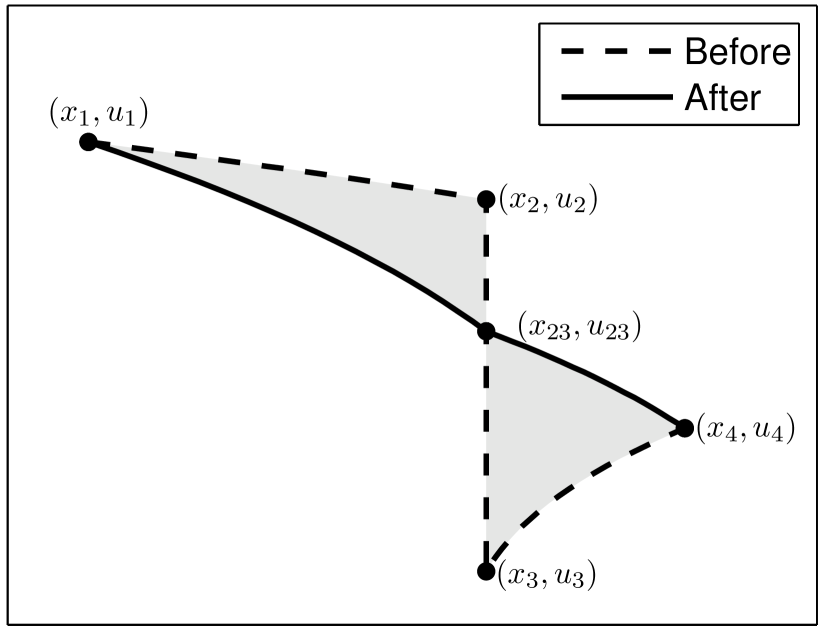
Figure 1: Merging two particles

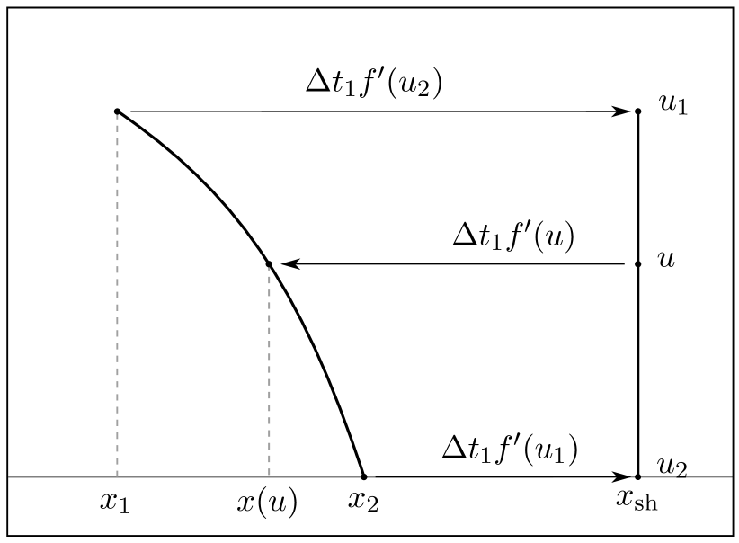
Figure 2: Definition of the interpolation

4.2 Conservative Interpolation

The particle management does not require an interpolation between points. As it stands, it complements the characteristic movement to yield a full particle method for the conservation law (1) that can run for arbitrarily long times. Yet, for plotting the solution and interpreting approximation properties, it is desirable to define an interpolation that is compatible with the conservation principles of the underlying partial differential equation. We define such an interpolation between each two neighboring points $(x_{1},u_{1})$ and $(x_{2},u_{2})$.

In the case $u_{1}=u_{2}$, we define the interpolation to be a constant. In the following, we describe the case $u_{1}\neq u_{2}$. Assume that $f$ is strictly convex or concave in $[u_{1},u_{2}]$. Therefore $f^{\prime}(u_{1})\neq f^{\prime}(u_{2})$. Hence, as derived in Sect. 2.1, the solution either came from a discontinuity (i.e. it is a rarefaction) or it will become a shock. The time $\varDelta t_{1}$ until this discontinuity happens is given by (8). At time $t+\varDelta t_{1}$ the points have the same position $x_{1}=x_{2}=x_{\text{sh}}$, as shown in Fig. 2. At this time the interpolation must be a straight line connecting the two points, representing a discontinuity at $x_{\text{sh}}$. We require any point of the interpolating function $(x,u)$ to move with its characteristic velocity $f^{\prime}(u)$ in the time between $t$ and $t+\varDelta t_{1}$. This defines the interpolation uniquely as

$$x(u)=x_{1}-t_{1}\left(f^{\prime}(u)-f^{\prime}(u_{1})\right)=x_{1}+\frac{f^{\prime}(u)-f^{\prime}(u_{1})}{f^{\prime}(u_{2})-f^{\prime}(u_{1})}(x_{2}-x_{1})\;.$$ (13)

Defining $x$ as a function of $u$ is in fact an advantage, since at a discontinuity characteristics for all intermediate values $u$ are defined. Thus, rarefaction fans arise naturally if $f^{\prime}(u_{1})<f^{\prime}(u_{2})$. Since $f^{\prime\prime}$ has no inflection points between $u_{1}$ and $u_{2}$, the inverse function $u(x)$ exists. However, it is only required at a single point for particle management. For plotting purposes we can always plot $x(u)$ instead.

Lemma 4

The interpolation (13) is a solution of the conservation law (1).

Proof

Using that $\dot{x}_{i}(t)=f^{\prime}(u_{i})$ for $i=1,2$ one obtains

$$\frac{\partial x}{\partial t}(u,t) =\dot{x}_{1}+\frac{f^{\prime}(u)-f^{\prime}(u_{1})}{f^{\prime}(u_{2})-f^{\prime}(u_{1})}(\dot{x}_{2}-\dot{x}_{1})$$

$$=f^{\prime}(u_{1})+\frac{f^{\prime}(u)-f^{\prime}(u_{1})}{f^{\prime}(u_{2})-f^{\prime}(u_{1})}(f^{\prime}(u_{2})-f^{\prime}(u_{1}))=f^{\prime}(u)\;.$$

Thus every point on the interpolation $u(x,t)$ satisfies the characteristic equation (2).∎

Corollary 2 (exact solution property)

Consider characteristic particles with $x_{1}(t)<x_{2}(t)<\dots<x_{n}(t)$ for $t\in[t_{1},t_{2}]$. At any time consider the function defined by the interpolation (13). This function is a classical (i.e. continuous) solution to the conservation law (1). In particular, it satisfies the conservation properties given in Sect. 2.1.

Theorem 4.3 (TVD)

With the assumptions of Theorem 4.1, the particle method is total variation diminishing.

Proof

Due to Corollary 2, the characteristic movement yields an exact solution, thus the total variation is constant. Particle insertion simply refines the interpolation, thus preserves the total variation. Due to Theorem 4.1, merging of particles yields a new particle with a function value $u_{23}$ between the values of the removed particles. Thus, the total variation is the same as before the merge or smaller.∎

Remark 1

The method is particularly efficient for quadratic flux functions. In this case the interpolation (13) between two points is a straight line, since $f^{\prime}$ is linear. Furthermore, the average (7) is the arithmetic mean $a(u_{1},u_{2})=\frac{u_{1}+u_{2}}{2}$, since $f^{\prime\prime}$ is constant. Consequently, the function values for particle insertion and merging can be computed explicitly.

Remark 2

The method has some similarity to front tracking by Holden et al. seibold::HoldenHoldenHeghKrohn1988 , and some fundamental differences. In front tracking, one approximates the flux function by a piecewise linear, and the solution by a piecewise constant function. Shocks are moved according to the Rankine-Hugoniot condition. In comparison, our method uses the wave solutions. Hence, in front tracking everything is a shock; in the particle method, everything is a wave.

5 Entropy

We have argued in Sect. 4.2 that due to the constructed interpolation the particle method naturally distinguishes shocks from rarefaction fans. In this section, we show that the method in fact satisfies the entropy condition

$$\eta(u)_{t}+q(u)\leq 0$$ (14)

if a technical assumption on the resolution of shocks is satisfied. We consider the Kružkov entropy pair $\eta_{k}(u)=\left|u-k\right|$, $q_{k}(u)={\rm sign}(u-k)(f(u)-f(k))$. As argued by Holden et al. seibold::HoldenRisebro2002 , if (14) is satisfied for $\eta_{k}$, then it is satisfied for any convex entropy function. Relation (14) implies that the total entropy $\int\eta_{k}(u(x))\,\mathrm{d}x$ does not increase in time for all values of $k$. Using the interpolation (13) we show that the numerical solution obtained by the particle method satisfies this condition.

Lemma 5 (entropy for merging)

Consider four particles located at $x_{1}<x_{2}=x_{3}<x_{4}$, with the middle two to be merged. We consider the case $f^{\prime\prime}>0$, i.e. $u_{2}>u_{3}$ WLOG. If the resulting value $u_{23}$ satisfies $u_{1}\geq u_{23}\geq u_{4}$, then the Kružkov entropy does not increase due to the merge.

Proof

We consider the segment $[x_{1},x_{4}]$. Let $u(x)$ and $\tilde{u}(x)$ denote the interpolating function before resp. after the merge. The area under the function is preserved. We present the proof for $k\leq u_{23}$. For $k\geq u_{23}$ the proof is similar. The interpolating function $u$ is monotone in the value of its endpoints, thus $u(x)\leq\tilde{u}(x)$ for $x\in[x_{2},x_{4}]$. Since $\left|x\right|=x-2\varTheta(-x)$, where $\varTheta(x)$ is the Heaviside step function, we can write

$$\int_{x_{1}}^{x_{4}}\!\left|u\!-\!k\right|\,\mathrm{d}x =\int_{x_{1}}^{x_{4}}\!\left(u\!-\!k\right)\,\mathrm{d}x-2\int_{x_{1}}^{x_{4}}\!(u\!-\!k)\varTheta(k\!-\!u)\,\mathrm{d}x$$

$$=\int_{x_{1}}^{x_{4}}\!\left(\tilde{u}\!-\!k\right)\,\mathrm{d}x-2\int_{x_{2}}^{x_{4}}(u\!-\!k)\varTheta(k\!-\!u)\,\mathrm{d}x$$

$$\geq\int_{x_{1}}^{x_{4}}\!\left(\tilde{u}\!-\!k\right)\,\mathrm{d}x-2\int_{x_{2}}^{x_{4}}(\tilde{u}\!-\!k)\varTheta(k\!-\!u)\,\mathrm{d}x\geq\int_{x_{1}}^{x_{4}}\!\left|\tilde{u}\!-\!k\right|\,\mathrm{d}x\;.$$

Thus, the entropy does not increase due to the merge.∎

The assumption of Lemma 5 implies that shocks must be reasonably well resolved before the points defining it are merged. It is satisfied if left and right of a shock points are not too far away. In the method, it can be ensured by an entropy fix: A merge is rejected a posteriori if the resolution condition is not satisfied. Then, points are inserted near the shock, and the merge is re-attempted. It remains to show in future work that with this procedure Theorem 4.2 still holds.

Theorem 5.1

The presented particle method yields entropy solutions.

Proof

During the characteristic movement of the points the entropy is constant, since due to Corollary 2 the interpolation is a classical solution to the conservation law. Particle insertion does not change the interpolation, thus it does not change the entropy. Merging does not increase the entropy if the conditions of Lemma 5 are satisfied.∎

6 Numerical Results

The particle method is particularly well suited for initial conditions that are composed of similarity solutions. By construction, the movement of the particles yields the exact solution as long as the solution is smooth. General initial conditions can be approximated by the interpolation (13). Good strategies of sampling initial conditions shall be addressed in future work. Figure 3 shows a smooth initial function $u_{0}(x)=\exp\left(-x^{2}\right)\cos\left(\pi x\right)$ and its time evolution under the flux function $f(u)=\frac{1}{4}u^{4}$. The curved shape of the interpolation is due to the nonlinearity in $f^{\prime}$. At time $t=0.25$ the solution (obtained by CLAWPACK using 80000 points) is still smooth, and thus represented exactly on the particles. At time $t=8$ shocks and rarefactions have occurred and interacted. Although the numerical solution uses only a few points, it represents the true solution well.

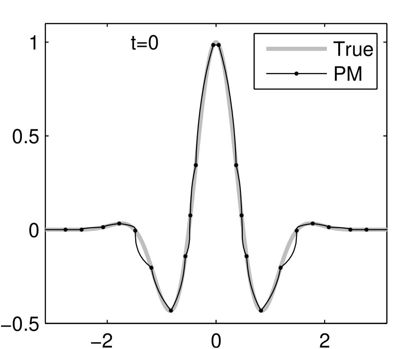
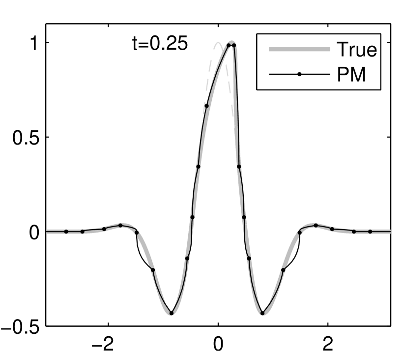
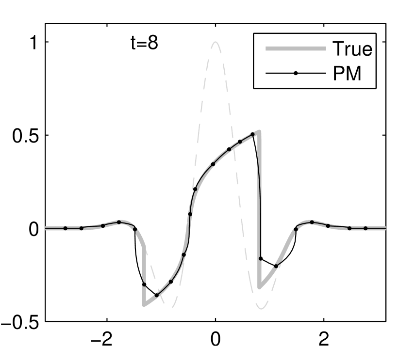
Figure 3: The particle method for $f(u)=\tfrac{1}{4}u^{4}$ before and after a shock

The accuracy of the particle method is measured numerically. We consider the flux function and initial conditions as used in Fig. 3. For a sequence of resolutions $h$, the initial data are sampled, and the particle method is applied ($d_{\text{m}ax}=1.9h$). Figure 4 shows the $L^{1}$-error to the correct solution (obtained by a computation with much higher resolution, verified with CLAWPACK). While the solution is smooth ($t=0.25$), the method is second order accurate, as is sampling the initial data. After a shock has occurred ($t=0.35$), the approximate solution (dots) becomes only first order accurate, since the shock has just been treated by particle management, thus an error of the order height$\times$width of the shock is made. A postprocessing step (squares) can recover the second order accuracy: At merged particles, discontinuities are placed so that the total area is preserved.

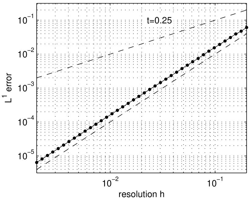
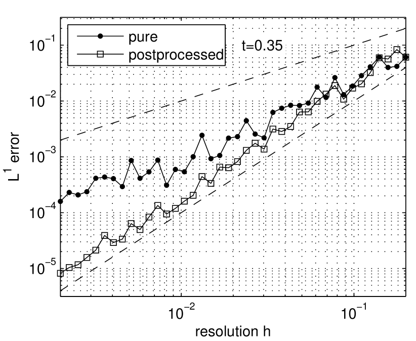
Figure 4: Error to the correct solution before and after a shock

7 Non-Convex Flux Functions

So far we have only considered flux functions with no inflection points (i.e. $f^{\prime\prime}$ has always the same sign) on the region of interest. In this section, we generalize to flux functions for which $f^{\prime\prime}$ has a finite number of zero crossings $u^{*}_{1}<\dots<u^{*}_{k}$. Between two such points $u\in[u^{*}_{i},u^{*}_{i+1}]$ the flux function is either convex or concave. We impose the following requirement for any set of particles: Between any two neighboring particles for which $f^{\prime\prime}$ has opposite sign, there must be an inflection particle $(x,u_{i}^{*})$. Thus, between two neighboring particles, $f$ has never an inflection point, and most results from the previous sections apply. The interpolation between any two particles is uniquely defined by (13). It has infinite slope at the inflection points, but this is harmless. The characteristic movement of particles is the same as for flux functions without inflection points. The only complication is merging of particles when an inflection particle is involved: The standard approach, as presented in Sect. 4.1, removes two colliding points and replaces them with a point of a different function value. If an inflection particle is involved in a collision, we must merge points in a different way so that an inflection particle remains.

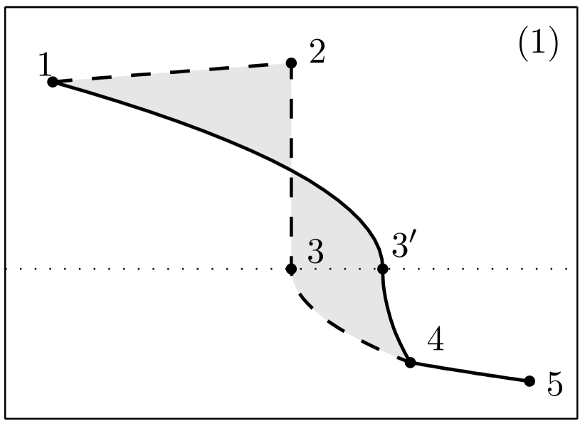
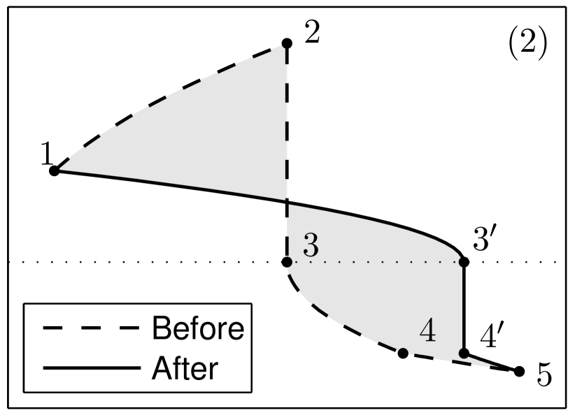
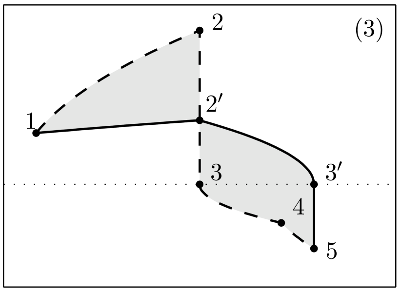
Figure 5: Particle management around an inflection particle ($f^{\prime\prime}(u_{3})=0$)

We present one such special merge for dealing with a single inflection point (we do not consider here the interaction of two inflection points). Also, we only consider a collision where the positions are exactly the same. Since the inflection particle must remain (although its position may change), we consider five neighboring particles and not four as before. Let $(x_{i},u_{i}),i=1,\ldots,5$ be these particle so that $x_{2}=x_{3}$, $f^{\prime\prime}(u_{3})=0$, and (WLOG) $f^{\prime\prime\prime}>0$, i.e. the inflection particle is the slowest. The other cases are simple symmetries of this situation. We present three successive steps to finding the final configuration of the particles. Each next step is attempted if the previous one failed.

1. Remove particle 2 and increase $x_{3}$ to satisfy the area condition. This fails if $x_{3}$ needs to be increased beyond $x_{4}$.

2. Remove particle 2, set $x_{3}=x_{4}$ and increase both to satisfy the area condition. This fails if $x_{3},x_{4}$ need to be increased beyond $x_{5}$.

3. Remove particle 4, set $x_{3}=x_{5}$ and find $u_{2}$ to satisfy the area condition. This cannot fail if the previous two have failed.

Formally, the resulting configuration could require another, immediate, merge (since $x_{3}=x_{4}$ or $x_{3}=x_{5}$). However, we need not merge these points as they move away from each other. The five point particle management guarantees that in each merging step one particle is removed, thus Theorem 4.2 holds.

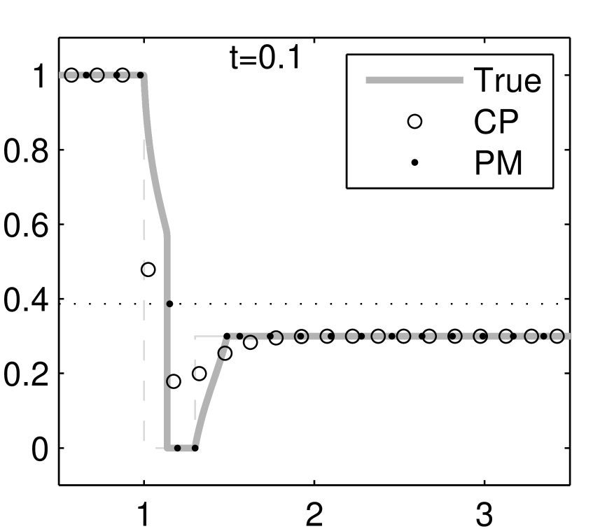
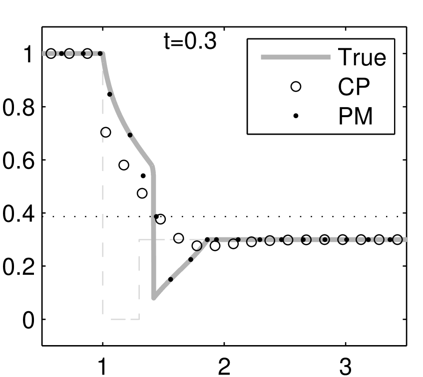
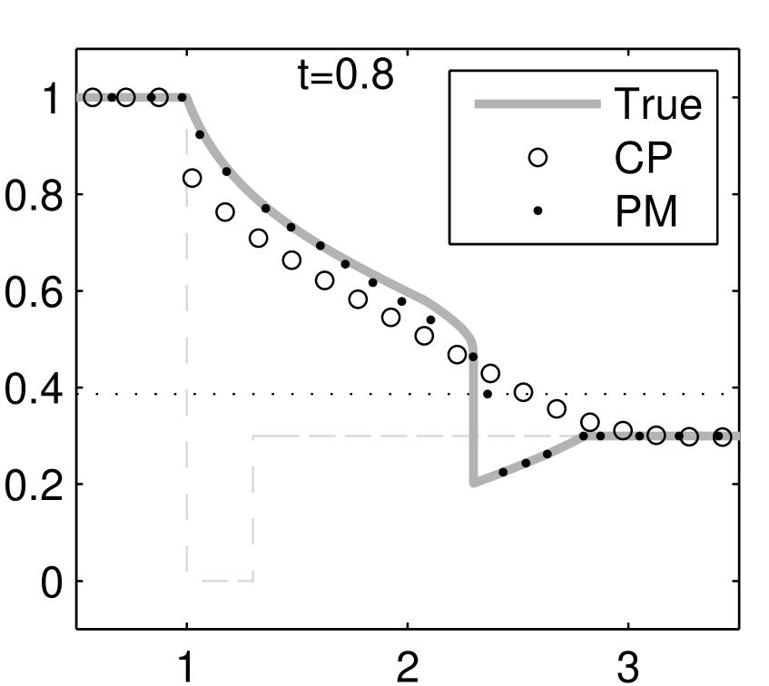
Figure 6: Numerical results for the Buckley-Leverett equation

As numerical evidence of the performance, we apply our method to the Buckley-Leverett equation (see LeVeque seibold::LeVeque2002 ), defined by the flux function $f(u)=\frac{u^{2}}{u^{2}+\frac{1}{2}(1-u)^{2}}$. It is a simple model for two-phase fluid flow in a porous medium. We consider piecewise constant initial data with a large downward jump crossing the inflection point, and a small upward jump. The large jump develops a shock at the bottom and a rarefaction at the top, the small jump is a pure rarefaction. Around $t=0.2$, the two similarity solutions interact, thus lowering the separation point between shock and rarefaction. Figure 6 shows the reference solution (solid line, by CLAWPACK using 80000 points). The solution obtained by our particle method (dots) is compared to a second order CLAWPACK solution (circles) of about the same resolution. While the finite volume scheme loses the downward jump very quickly, the particle method captures the behavior of the solution almost precisely. Only directly near the shock inaccuracies are visible, which are due to the crude resolution. The solution away from the shock is nearly unaffected by the error at the shock. Note that although we impose a special treatment only at the inflection point, the switching point between shock and rarefaction is identified correctly.

8 Conclusions and Outlook

We have presented a particle method for 1D scalar conservation laws, which is based on the characteristic equations. The associated interpolation yields an analytical solution wherever the solution is smooth. Particle management resolves the interaction of characteristics locally while conserving area. Thus, shocks are resolved without creating any numerical dissipation away from shocks. The method is TVD and entropy decreasing, and shows second-order accuracy. It deals well with non-convex flux functions, as the results for the Buckley-Leverett equation show. The particle method serves as a good alternative to fixed grid methods whenever 1D scalar conservation laws have to be solved with few degrees of freedom, but exact conservation and sharp shocks are desired. An application, which we plan to investigate in future work, is nonlinear flow in networks (e.g. traffic flow in road networks). For large networks, only a few number of unknowns can be devoted to the numerical solution on each edge. We regard the current work as a first step towards a more general particle method. Future work will focus on three main directions:

• Source terms: Source terms in an equation $u_{t}+\left(f(u)\right)_{x}=g(x,u)$ could be handled using a fractional step method: In each time step, we would first move the particles according to $u_{t}+\left(f(u)\right)_{x}=0$ (including particle management), then change their values according to an integral formulation of $u_{t}=g(x,u)$. In the latter step, the constructed interpolation can be used.

• Systems of conservation laws: The particle method is based on similarity solutions of the conservation law. For simple systems, such as the shallow water equations in 1D, the analytical solutions to Riemann problems are known. Two complications arise in the generalization of the method:

  • To connect two general states in a hyperbolic system, intermediate states have to be included.

  • For a general system it is not clear at which velocity to move the particles.

• Higher space dimensions: Scalar conservation laws in higher space dimensions can be reduced to 1D problems to be solved by fractional steps. In principle, this dimensional splitting can be used with the particle method. However, remeshing would be required between the different spacial directions, thus the benefits of the meshfree approach would be lost. For the generalization to a fundamentally meshfree approach in higher space dimensions, the following problem has to be overcome: In 1D one is never truly meshfree, since the points have a natural ordering. The method uses this in the interpolation and to detect shocks. In 2D/3D shocks can occur without particles colliding, as they can move past each other. Other meshfree methods, such as FPM applied to the Euler equations, circumvent this issue by using the pressure to regulate shocks.

References

- (1) A. J. Chorin, Numerical study of slightly viscous flow, J. Fluid Mech. 57 (1973), 785–796.
- (2) R. Courant, E. Isaacson, and M. Rees, On the solution of nonlinear hyperbolic differential equations by finite differences, Comm. Pure Appl. Math. 5 (1952), 243–255.
- (3) G. A. Dilts, Moving least squares particles hydrodynamics I, consistency and stability, Internat. J. Numer. Methods Engrg. 44 (1999), 1115–1155.
- (4) L. C. Evans, Partial differential equations, Graduate Studies in Mathematics, vol. 19, American Mathematical Society, 1998.
- (5) R. A. Gingold and J. J. Monaghan, Smoothed particle hydrodynamics – Theory and application to nonspherical stars, Mon. Not. R. Astron. Soc. 181 (1977), 375.
- (6) A. Harten, B. Engquist, S. Osher, and S. Chakravarthy, Uniformly high order accurate essentially non-oscillatory schemes. III, J. Comput. Phys. 71 (1987), no. 2, 231–303.
- (7) H. Holden, L. Holden, and R. Hegh-Krohn, A numerical method for first order nonlinear scalar conservation laws in one dimension, Comput. Math. Appl. 15 (1988), no. 6–8, 595–602.
- (8) H. Holden and N. H. Risebro, Front tracking for hyperbolic conservation laws, Springer, 2002.
- (9) J. Kuhnert and S. Tiwari, A meshfree method for incompressible fluid flows with incorporated surface tension, Revue aurope’enne des elements finis 11 (2002), no. 7–8, 965–987.
- (10) R. J. Le Veque, Finite volume methods for hyperbolic problems, first ed., Cambridge University Press, 2002.
- (11) T. Liszka and J. Orkisz, The finite difference method at arbitrary irregular grids and its application in applied mechanics, Comput. & Structures 11 (1980), 83–95.
- (12) X.-D. Liu, S. Osher, and T. Chan, Weighted essentially non-oscillatory schemes, J. Computat. Phys. 115 (1994), 200–212.
- (13) L. Lucy, A numerical approach to the testing of the fission hypothesis, Astronomical Journal 82 (1977), 1013–1024.
- (14) B. van Leer, Towards the ultimate conservative difference scheme II. Monotonicity and conservation combined in a second order scheme, J. Computat. Phys. 14 (1974), 361–370.