Parameters and Predictions for the Long-Period Transiting Planet HD 17156b

Abstract

We report high-cadence time-series photometry of the recently-discovered transiting exoplanet system HD 17156, spanning the time of transit on UT 2007 October 1, from three separate observatories. We present a joint analysis of our photometry, previously published radial velocity measurements, and times of transit center for 3 additional events. Adopting the spectroscopically-determined values and uncertainties for the stellar mass and radius, we estimate a planet radius of $R_{p}=1.01\pm 0.09\,R_{\rm Jup}$ and an inclination of $i=86.5^{+1.1}_{-0.7}$ degrees. We find a time of transit center of $T_{c}=2454374.8338\pm 0.0020$ HJD and an orbital period of $P=21.21691\pm 0.00071$ days, and note that the 4 transits reported to date show no sign of timing variations that would indicate the presence of a third body in the system. Our results do not preclude the existence of a secondary eclipse, but imply there is only a 9.2% chance for this to be present, and an even lower probability (6.9%) that the secondary eclipse would be a non-grazing event. Due to its eccentric orbit and long period, HD 17156b is a fascinating object for the study of the dynamics of exoplanet atmospheres. To aid such future studies, we present theoretical light curves for the variable infrared emission from the visible hemisphere of the planet throughout its orbit.

1. Introduction

Twenty-eight transiting planets are now reported in the literature, and the doubling time scale for new detections is now roughly one year. As reviewed by Charbonneau et al. (2007), it is these objects that have allowed the study of the physical structure and atmospheric chemistry and dynamics of gas giant exoplanets, and opened the field of comparative exoplanetology. However, the majority have orbital periods of a few days, due both to the lower geometric probability of transits occurring as the orbital period increases, and due to the limitations of ground-based photometric transit surveys that strongly favor detection of short-period systems. The latter problem can be circumvented by searching for transits of known radial velocity planet-bearing stars, putting to use the radial velocity information to constrain the possible time of transit. This is the primary aim of the Transitsearch.org network (Seagroves et al., 2003), which, starting in 2002, has been conducting photometric follow-up observations of known radial velocity detected planets. This network is a prime example of successful collaboration between amateur and professional astronomers.

Although longer period planets possess a lower geometric probability to transit, there exists a loop-hole for some planets on highly eccentric orbits. The transit probability for a planet on an eccentric orbit, with periastron near inferior conjunction, is amplified by a factor

$$A=\left[{{1+e\cos(\frac{\pi}{2}-\omega)}\over{1-e^{2}}}\right]$$ (1)

where $e$ is the eccentricity, and $\omega$ is the argument of pericenter (Seagroves et al., 2003). An amplification factor near 2.9 for the planet orbiting HD 17156 (Fischer et al., 2007), along with an extremely short time window for possible transits, brought the system to the attention of the Transitsearch.org network. This was rewarded by the detection of transits as recently announced by Barbieri et al. (2007).

This unique system contains a $3.1$-$M_{\rm Jup}$ transiting planet in a $21.2$ day highly-eccentric orbit ($e=0.67$) about a bright ($V=8.2$) G0V star. Gillon et al. (2007) have recently presented refined estimates of the system parameters based on new photometric data. Even among planets with periods beyond 5 days, where the timescale for tidal circularization quickly grows to exceed the age of most systems, HD 17156b’s eccentricity is unusually high, thus making it an interesting test case for models of planetary migration. Preliminary measurements of the Rossiter-McLaughlin effect (Rossiter, 1924; McLaughlin, 1924; Gaudi & Winn, 2007; Winn, 2007) by Narita et al. (2007) show evidence for a misalignment between the stellar spin axis and the planetary orbit axis, which may indicate a migration mechanism involving planet-planet scattering (see e.g. Chatterjee et al., 2007), or Kozai migration under perturbation by a yet undetected stellar companion or second planet (Fabrycky & Tremaine, 2007; Wu, Murray & Ramsahai, 2007). The large eccentricity and long period also make HD 17156 a particularly attractive target for several additional follow-up studies. First, it presents a unique opportunity for the study of the structure and dynamics of a gas-giant atmosphere under strongly varying illumination, through infrared monitoring of the planetary emission (e.g. Harrington et al. 2006; Cowan et al. 2007; Knutson et al. 2007a, b). Second, by monitoring successive times of transit, the presence of additional bodies in the system can be detected or constrained from the resulting perturbations on the orbit of HD 17156b (Holman & Murray 2005; Agol et al. 2005; Steffen & Agol 2005).

The purpose of our paper is three-fold: First, we seek to refine the estimates of the system parameters that were only poorly constrained by the light curves of Barbieri et al. (2007). Second, we document the time of center of transit and search for transit timing variations. Third, we evaluate the likelihood that a secondary eclipse will be observable for HD 17156, and present theoretical predictions of the infrared phase variations as might be detected with the Spitzer Space Telescope. We elected to perform an independent analysis from that of Gillon et al. (2007), and therefore do not use their orbital parameters as constraints, since at the time of writing these are still subject to change as their paper has not yet been accepted for publication. We do however make use of the time of mid-transit presented in their Table 1.

We begin by presenting a description of our observations of the transit event on UT 2007 October 1 in §2. We then present our combined analysis of the extant radial velocity measurements (§3) and photometric data (§4), and our resulting estimates of the system parameters and likelihood of a secondary eclipse. In §5, we compare our constraints on the planet mass and radius with planetary structural models, summarize the current constraints on the presence of transit timing variations in the system, and present model predictions for the planetary infrared light curve. We conclude in §6 with a discussion of compelling avenues for future research.

2. Observations

Using the orbital period given by Fischer et al. (2007) and the time of mid-transit measured by Barbieri et al. (2007), we predicted that an event would occur on UT 2007 October 1 with transit center at UT 7:53, which was well-situated for observatories in the southwestern United States. We present below a description of the data we gathered from three such observatories, and summarize the calibration of the raw frames and extraction of the time series for each.

2.1. Mount Laguna Observatory

We observed HD 17156 with the Smith 0.6 m telescope at Mount Laguna Observatory using a Bessell $R$ filter and an SBIG STL-1001E CCD camera (giving a scale of $0\farcs 4$/pixel at the $f/20$ Cassegrain focus), using BD+71 168 ($V=9.57$, B8 spectral type) as our local comparison star. The integration time for each exposure was 4 s, with a 4.3s readout time and a net cadence of 8.3 s. For each frame, we calculated the time at mid-exposure and corrected this time to heliocentric Julian Day. We dark-subtracted and flat-fielded the raw images in IRAF, and then performed aperture photometry using a circular aperture with radius 12.8 arcsec. The use of the large aperture insulated our analysis against seeing-induced aperture losses, as the seeing varied from 2.1 arcsec to 2.7 arcsec over the course of the night. Clouds were present at several times during the observations, especially after mid-transit. To avoid systematic effects due to cloud-induced differential extinction of the different color stars, we rejected observations for which the calibration star showed more than $8\%$ light loss. The resulting 2148 points were binned 20:1 and uncertainties were estimated from the RMS scatter in each bin divided by $\sqrt{20}$. Typical uncertainties for the binned points were $0.3-0.7\%$.

2.2. Torrance California

We observed a field centered on HD 17156 using a commercial $0.25$m Meade LX200 telescope and a Meade Deep Sky Imager Pro II CCD camera. We employed an f/3.3 focal reducer to increase the field-of-view to $\sim 20\times 30$ arcmin. We gathered $10\,345$ exposures through an Edmund Optics IR-pass filter (approximating the conventional $I$-band), between UT 4:20 and 13:25. The integration time for each image was 2 s. Weather conditions were clear. Approximately $10\%$ of the frames were lost due to an intermittent issue with the CCD readout, and due to wind shake, and the guide star was lost temporarily at 6:10 UT, resulting in a large pointing shift ($\sim 5\ {\rm arcmin}$).

These images were processed using the software described in Irwin et al. (2007), which was originally developed for the Monitor project (Aigrain et al., 2007). Individual frames were processed by subtracting a master dark and dividing by a master flat field. We then ran the pipeline source detection software (see Irwin et al. 2007) on all of the data frames, choosing a single frame taken in good conditions for use as a reference. For each image, we derived an astrometric solution employing an implementation of the triangle matching algorithm of Groth (1986) to cope with shifts in the telescope position (these were $\sim 10$ pixels peak-to-peak, in a periodic fashion, presumably due to errors in the telescope worm drives), and field rotation due to polar misalignment of the mount.

We generated light curves using the method described in Irwin et al. (2007), using the nearby star BD+71 168 as the comparison source for the differential photometry. We found that the normalized time series data gathered before and after the large image motion at UT 6:10 have an photometric offset of roughly 3%. Since the data obtained before UT 6:10 were well before the ingress, we simply trimmed them from the time-series; similarly, we trimmed the data that occurred more than 0.2 days after the transit midpoint. We also trimmed single large outliers by identifying all points that deviated from the median of the time-series by more than 8%. The typical photometric errors in the final, trimmed time-series are 2% per data point, as determined from the RMS variation from the data gathered after egress. We then binned this time series by a factor of 15 (and assumed that the errors in the binned data were reduced according to Poisson statistics); this binning was necessary to keep the computational time for the model fitting (§4) to a manageable duration, but the binning did not degrade the quality of the fits.

2.3. Las Cumbres Observatory Global Telescope

We also observed the event using a $0.4$m Meade RCX400 telescope on a custom mount, temporarily located in the car park of the Las Cumbres Observatory Global Telescope (LCOGT) offices in Goleta, California. We used an SBIG STL-6303E CCD camera to image a $20\times 30$ arcmin field with 0.6-arcsec pixels. 380 useful images were taken between UT 5:30 and 11:00, with the airmass decreasing from 1.6 to a minimum of 1.25 near UT 10:00. No autoguiding was used, and the field drifted by $\sim 100$ arcsec during the run. The observations were made through the “Red” filter from the LRGBC filter set provided with the camera by SBIG, with $\sim 90$% transmission in the range 580–680 nm. Exposure times varied from 20 to 30 seconds. The readout time was 22 seconds. The telescope was defocused to avoid saturating the target star, which was the brightest in the field. The amount of defocus was increased at about UT 06:30, shortly before the transit ingress, but this did not significantly affect the relative photometry at that point.

Bias and dark subtraction and flat fielding were done using standard IRAF tasks. HD 17156 and ten reference stars were measured using the DAOPHOT aperture photometry package, with apertures of radius 10.6 arcsec. The light curve was divided by the average of the reference light curves to remove the effects of varying atmospheric extinction and focus changes. The standard deviation of the (unbinned) points outside the transit was 0.4%.

The scatter of these data is lower than for the Mount Laguna $0.6$m observations, despite the smaller aperture, since the larger field-of-view permits the use of multiple comparison stars. In the Mount Laguna data, the signal-to-noise ratio of the final light curve was limited by that of the comparison light curve, due to the use of a comparison star fainter than the target. By using multiple comparison stars for the Las Cumbres data, it was possible to attain a higher signal level in the comparison light curve, such that the overall noise was dominated by the target, hence giving a net overall improvement in signal-to-noise ratio despite the use of a smaller aperture telescope. Observing conditions were also somewhat worse at Mount Laguna, and this along with the use of defocus to render the observations insensitive to seeing variations, and to average out pixel-to-pixel flat fielding errors, also contribute to reducing the noise level in the Las Cumbres data.

3. Analysis of the Radial Velocity Data

Our orbital model was obtained by jointly fitting the Fischer et al. (2007) radial velocity data (converted to HJD) in conjunction with the following four observed central transit times, numbered $N=-1,0,2,3$ (where we denote our observation on UT 2007 October 1 as event $N=0$): $T_{c,-1}={\rm HJD}\,2454353.61\pm 0.02$ (Barbieri et al., 2007), $T_{c,0}={\rm HJD}\,2454374.8338\pm 0.0020$ (this paper; see §4), $T_{c,2}={\rm HJD}\,2454417.2645\pm 0.0021$ (Narita et al., 2007), and $T_{c,3}={\rm HJD}\,{2454438.4835}^{+0.0009}_{-0.0025}$ (Gillon et al., 2007).

For a Keplerian orbit, the instantaneous stellar radial velocity is given by $V_{{\rm mod},i}=K\,[\cos(f_{i}+\omega)+e\,\cos\omega]$, where $f_{i}$ is the true anomaly of the planet at time $t_{i}$. If we assume an edge-on orbit, the time of central transit occurs when $f_{t}={\pi/2}-\omega$. Given the precision of the available photometry, this approximation to $f_{t}$ is excellent. The true anomaly, $f$, is in turn related to the the eccentric anomaly, $E$, via $E=2\arctan{\sqrt{(1-e)/(1+e)}\tan(f/2)}$, so that a central transit, $T_{c,i}$, occurs at a fixed interval $\Delta T=P(E-e\sin{E})/{2\pi}$ following the epoch of a periastron passage, $T_{p,i}$.

Given $N_{RV}$ radial velocity measurements (here, $N_{RV}=33$) and $N_{T_{c}}$ central transit measurements, the goodness-of-fit function of a particular orbital model is calculated as:

$$\chi^{2}=\sum_{i=1}^{N_{RV}}\left({V_{{\rm mod},i}-V_{{\rm obs},i}\over{\sigma_{i}}}\right)^{2}+\sum_{i=0}^{N_{Tc}}\left({T_{p,i}+\Delta T-T_{c,i}\over{\sigma_{i}}}\right)^{2}$$ (2)

We use a Levenberg-Marquardt algorithm to minimize $\chi^{2}$. The best-fitting orbital parameters are listed in Table 1. To obtain the quoted uncertainties, a simple bootstrap procedure was used. An aggregate of 1000 alternate datasets was created by (1) redrawing the radial velocities with replacement, and (2) sampling $T_{c}$ values for the four transits by drawing from the Gaussian distributions implied by the quoted errors. Fits to each of these data sets were obtained, and the resulting distributions of orbital parameters were used to derive the $68.3\%$ confidence intervals for each parameter. In Table 1, we have also given in brackets the standard deviations of these parameter distributions. The latter are larger than the former due to the existence of outliers in the bootstrap sample. These are generated because the relative importance of each radial velocity data point in constraining the derived orbital parameters depends on the orbital phase as a result of the highly eccentric orbit: the points close to periastron have the largest effect on the fit. Consequently, when the bootstrapping procedure exchanges a point close to periastron, the parameters estimated from this particular realization of the procedure show sizable variations. We therefore prefer the $68.3\%$ confidence intervals, since these are robust to the presence of the outliers, which are in turn the result of the bootstrap procedure not being strictly applicable to data such as these which are not independent and identically-distributed.

Table 1 Fitted Parameters for HD 17156.

Parameter	Value
$P$	$21.21691\pm 0.00071\ (0.00094)\ {\rm d}$
$e$	$0.670\pm 0.006\ (0.020)$
${\omega}$	$121{\fdg}3\pm 0{\fdg}9\ (1{\fdg}8)$
$K$	$273.8\pm 3.4\ (16.3)\ {\rm m\,s^{-1}}$
$T_{p}$	$2453738.605\pm 0.024\ (0.036)\ {\rm HJD}$
$T_{c}$	$2454374.8338\pm 0.0020\ {\rm HJD}$
$i$	$86{\fdg}5^{+1\fdg 1}_{-0{\fdg}7}$
$R_{p}/R_{\star}$	$0.070\pm 0.003$
$R_{p}$	$1.01\pm 0.09\ R_{\rm Jup}$
$R_{\star}$	$1.47\pm 0.08\ R_{\sun}$
$\rho$	$3.8^{+0.8}_{-1.1}$ g cm-3
$f_{1}$	$0.9989\pm 0.0025$
$k_{1}$	$-0.0006\pm 0.0015$
$f_{2}$	$1.006\pm 0.003$
$k_{2}$	$0.0049\pm 0.0022$
$c_{1}$	$-0.0024\pm 0.0005$
$c_{2}$	$0.0173\pm 0.0029$
$c_{3}$	$0.204\pm 0.064$

We note that the addition of the transit timing data provides a very strong constraint on the orbital period, but has only a minor effect on the other orbital parameters, which are in excellent agreement with the solution given by Fischer et al. (2007).

4. Photometric Analysis

We pooled together the three photometric data sets to fit a model light curve parametrized by the orbital and physical properties of the HD 17156 system. Our model incorporates 4 orbital parameters initially determined through the fit to the RV data: the period $P$, eccentricity $e$, time of periastron $T_{p}$, and argument of pericenter $\omega$. Given this orbit, we calculate a baseline light curve for a quadratically limb-darkened star (characterized by the stellar mass $M_{\star}$, radius $R_{\star}$, and 2 limb darkening coefficients for each photometric band pass) that is being occulted by a planet ($r_{p}=R_{p}/R_{\star}$) orbiting at an inclination $i$. To calculate the baseline light curve, we employ the analytic formulae of Mandel & Agol (2002), together with the quadratic limb-darkening coefficients tabulated by Claret (2000, 2004), for $T_{\mathrm{eff}}$ = 6000 K, [Fe/H] = $0.2$, $\log{g}=4.0$ (based on the stellar parameters given by Takeda et al. 2007). We adopted $R$-band coefficients for the Mount Laguna data, SDSS $r$-band coefficients for the Las Cumbres data, and $I$-band coefficients for the Torrance California data. In the latter two cases, the filters used for the observations only approximate $r$ and $I$, but the approximation is more than suitable for our purposes (in particular, the goodness-of-fit statistic described below is negligibly affected by errors in the assumed bandpass). The baseline flux is then modified by observational correction factors unique to each dataset (7 additional parameters described below).

Nominally, our model fixes $P$, $e$, $\omega$, 6 limb darkening coefficients, and $M_{\star}$, although we iteratively update the first three of these parameters as the RV fit is apprised of the transit timing resulting from the light curve fit. Ultimately, the change in these three parameters from the iterative update process had negligible effect on the quality of the light curve fit and had negligible consequences for the stellar and planetary properties determined by the transit analysis. Note that although $T_{p}$ is a fit-variable in our transit analysis, the value that is really being constrained by the photometry is the time of central transit, $T_{c}$, which is related to a degenerate combination of $P$, $e$, $\omega$, and $T_{p}$. We fix $M_{\star}$ to the value $1.2M_{\odot}$ (Fischer et al., 2007), which was determined by matching spectroscopic observations to stellar evolution tracks (Takeda et al., 2007). Here, the uncertainty in $M_{\star}$, for which the 95% confidence interval is $1.1-1.3\ M_{\odot}$, has only weak impact on the light curve fit. This is because, as described below, we adopt an external constraint on the stellar radius.

Our light curve model employed 11 free parameters: $T_{p}$, the planet-star radius ratio $r_{p}$, $R_{\star}$, $i$, and 7 additional parameters related to observational corrections. The Torrance and Mount Laguna fluxes were each multiplied by airmass corrections of the form $f\times\exp(-ka)$, where $f$ is a normalization factor, $a$ is the airmass, and $k$ is the extinction coefficient. We note, however, that including the Mount Laguna airmass correction had little effect on the quality of fit (indeed, the determined $f$ and $k$ were consistent with 1 and 0 respectively; see Table 1). We attempted the same airmass correction for the Las Cumbres data, but found that a quadratic function of time significantly improved the quality of fit. We adopted a $\chi^{2}$ function as our goodness-of-fit statistic, with an additional term reflecting a spectroscopic prior on $R_{\star}$, which is approximately Gaussian with $\sigma=0.085$ (G. Takeda, personal communication). This additional constraint proved necessary, as our data could not independently determine the stellar radius. The goodness-of-fit function is

$$\chi^{2}=\sum_{i}{\left(\frac{f_{mod}(i)-f_{obs}(i)}{\sigma_{i}}\right)^{2}}+\frac{(R_{\star}/R_{\sun}-1.47)^{2}}{0.085^{2}}$$ (3)

where $f_{mod}(i)$ is the calculated flux at the time of the $i^{th}$ data point, $f_{obs}(i)$ is the $i^{th}$ flux measurement, and $\sigma_{i}$ is the uncertainty of the $i^{th}$ flux measurement (derived as described for each data-set in §2). Using an IDL implementation of the amoeba algorithm (e.g. see Press et al. 1992), we performed an initial $\chi^{2}$ minimization over the space of free parameters in our model. Using the results, we then rescaled the $\sigma_{i}$ so that the reduced $\chi^{2}$ equals 1 separately for each dataset. We performed iterations of transit model fitting in conjunction with radial velocity fitting, using the derived transit timing to inform the radial velocity fit, which in turn updated the $P$, $e$, and $\omega$ used for the transit fit. As mentioned above, the parameter update had negligible effect on the derived stellar and planetary properties. The data, corrected for the airmass and instrumental effects, are shown in Figure 1 along with the best-fitting solution.

Figure 1.— Binned light curve of HD 17156, with the airmass and instrumental corrections described in §4 applied. Top: Mount Laguna $R$-band photometry. Middle: Las Cumbres photometry in a filter approximating $r$. Bottom: Torrance CA photometry in a filter approximating $I$. Dashed lines show the model fit simultaneously to the light curve and radial velocity data, as discussed in the text.

The uncertainty in the transit time was assessed by finely stepping $T_{p}$ through values near its best fitting value and calculating the minimum $\chi^{2}$ at each step, allowing the other free parameters to vary. The 1-$\sigma$ upper and lower limits were assessed by noting the $T_{p}$ values at which $\Delta\chi^{2}=1$. Given the other orbital parameters, we mapped each $T_{p}$ into the corresponding time of central transit, $T_{c}$. The resulting best fitting $T_{c}$ and uncertainties are reported in Table 1. Over the range of allowed $T_{p}$, we found very little correlation between it and the best fitting stellar/planetary parameters. For this reason, we decided to fix $T_{p}$ at its best fitting value for the Markov Chain Monte Carlo (MCMC) analysis described below. Note that by fixing $T_{p}$, the MCMC code only needs to perform a full Keplerian orbit calculation once, rather than at every step in the chain, thus dramatically speeding up the computation.

To estimate the uncertainty in the 10 remaining model parameters, we used an MCMC algorithm following the basic recipe described, for example, in Winn et al. (2007), with whom we share the terminology used below. We produced 10 chains, each of $10^{6}$ points, starting from independent initial parameter values. The “jump function” was tuned so that $\sim 25\%$ of jumps were executed, and the first $10\%$ of each chain was discarded to avoid the effect of the initial condition. We combined the chains, and in Table 1 we report the median value of each parameter, and assign uncertainties by taking the standard deviation of that parameter (except $i$, for which we report the $68.3\%$ confidence interval). In Figure 2, we show the results of this MCMC analysis. One of the major benefits of MCMC is that probability distributions for derived quantities, such as the secondary eclipse impact parameter (in the bottom right panel of Figure 2), are produced directly. Here, the impact parameter was taken to be the minimum projected separation between planet and star center in the units of the stellar radius.

Figure 2.— Posterior probability distributions for $R_{\star}$, the planet-star radius ratio, $R_{p}$, and the secondary eclipse impact parameter, based on $10^{7}$ MCMC samples. The secondary eclipse impact parameter is the minimum projected separation between planet and star center (near time of superior conjunction), in units of the $R_{\star}$. The dark shaded region shows where full secondary eclipses occur, while the light shaded region shows where grazing eclipses occur.

5. Discussion

5.1. Planetary mass, radius and density

The planet’s mass of $3.13\pm 0.11$ M_Jup (Fischer et al., 2007) is the third most massive among the known transiting planets, surpassed only by HD 147506b (8.6 $M_{\rm Jup}$; also known as HAT-P-2b; Bakos et al. 2007) and XO-3b (13.2 M_Jup; Johns-Krull et al. 2007). We find that the mean density of HD 17156 is $\rho=3.8^{+0.8}_{-1.1}$ g cm^-3, substantially higher than other transiting extrasolar planets, again with the exception of the remarkable planet HD 147506b ($\rho$=11.9 g cm^-3; Loeillet et al. 2007). HD 17156b begins to bridge the gap between HD 147506b and the other transiting planets.

The presence of a large rocky or metallic core has been suggested to account for “hot Jupiters” with high densities. For HD 17156b, the models of Bodenheimer et al. (2003) predict a radius of 1.11 $R_{\rm Jup}$ given the mass of HD 17156b, which is $\sim 1-\sigma$ larger than the radius derived from the light curve fitting, or equivalently, the measured density is higher than the models would predict. However, for such a massive planet, this discrepancy is difficult to resolve by invoking the presence of a solid core, since the dependence of planetary radius on the presence of a core is predicted to be very weak in this mass regime (e.g. Bodenheimer et al. 2003; Burrows et al. 2007; Fortney et al. 2007a). For example, Bodenheimer et al. (2003) predict that the addition of a 30 $M_{\earth}$ core reduces the radius by only $\sim$ 0.01 $R_{\rm Jup}$ for a $\sim$ 3 $M_{\rm Jup}$ planet. This scenario would therefore require an extremely massive core to account for the measured radius of HD 17156b.

Although a large rocky or metallic core can account for planets with high densities, the low density (i.e. large radius) planets such as TrES-4 (Mandushev et al., 2007) and WASP-1 (Collier Cameron et al., 2007) seem to defy explanation. One possible mechanism for keeping planetary radii from shrinking during planetary evolution is to pump energy into the planet via tidal interactions (e.g. Mardling 2007). Such orbital energy transfer mechanisms depend strongly on the orbital eccentricity, and HD 17156b represents a good test-case for these theories, having a significantly eccentric orbit ($e=0.67$). However, the radius of HD 17156b is not in any way exceptional when compared to the existing extrasolar planets with close to circular orbits. This leads one to speculate that tidal energy transfer via orbital dynamics may not play a substantial role in planetary radius evolution, or that in massive planets such as HD 17156b a mechanism is acting to allow the planets to more rapidly evolve to smaller radii. We note, however, that the recently-announced massive planet XO-3b (Johns-Krull et al., 2007) also has an eccentric orbit, but in contrast to HD 17156b, its radius is very large ($1.92R_{\rm Jup}$). Thus the challenges posed by newly-discovered exoplanets to theoretical models of their physical structure seem to continue unabated.

5.2. Search for transit timing variations

The availability of multiple measured times-of-transit allows the presence of additional bodies in the HD 17156 system to be detected or constrained, by searching for the influence of their gravitational perturbations on the orbit of HD 17156b (Holman & Murray 2005; Agol et al. 2005; Steffen & Agol 2005).

In Figure 3, we plot the observed minus calculated times of center of transit for the 4 events reported in the literature, including the event described in this paper. We find that these results do not yet reveal any evidence for timing variations that would indicate the presence of a third body in the system. Due to the long orbital period, HD 17156 may be more amenable to a search for such variations. However, the large orbital eccentricity implies a large region for which dynamical stability considerations would exclude the presence of such planets.

Figure 3.— Observed minus calculated times of transit for the four transit events discussed in this work. The dashed line shows the prediction assuming the values of $T_{c}$ and $P$ from Table 1. Since the value of $P$ was determined from a simultaneous fit to the transit times and radial velocity data, it does not represent the best fit to the transit times alone.

5.3. Prospects for infra-red observations

Our photometric analysis directly addresses the probability that HD 17156b undergoes secondary eclipse, which is only possible for certain combinations of $R_{\star}$ and $i$. We find a 9.2% chance for secondary eclipses to occur, but only a 6.9 % chance for non-grazing eclipses. If, indeed, HD 17156b undergoes eclipses, $i$ becomes locked rather tightly, thus greatly diminishing the allowed volume of parameter space for the stellar and planetary properties. Under this constraint, we find that the new best fitting values for ($i$,$R_{\star}$,$R_{p}$) are ($88{\fdg}7~{}^{+1{\fdg}0}_{-0{\fdg}1}$, $1.34\pm 0.03~{}R_{\odot}$, $0.89\pm 0.04~{}R_{\mathrm{Jup}}$). These considerations serve to motivate a search for the secondary eclipses.

HD 17156b’s large eccentricity leads to a 25-fold variation in received stellar flux over the course of the $21.2169\,{\rm d}$ orbital period. This dramatic variation in illumination should produce complex weather at the planet’s photosphere. In addition, the planet is subject to strong tidal forces during its periastron passage. The planet is therefore expected to be in pseudo-synchronous rotation, in which the planetary spin will be roughly synchronous with the orbit during the interval surrounding close approach. The theory of Hut (1981) predicts a pseudo-synchronous spin period, $P_{\rm spin}$ given by

$$P_{\rm spin}={1+{15\over{2}}e^{2}+{45\over{8}}e^{4}+{5\over{16}}e^{6}\over{(1+3e^{2}+{3\over{8}}e^{4})(1-e^{2})^{3/2}}}P_{\rm orbit}=91.3\,{\rm hr}$$ (4)

Knowledge of $P_{\rm spin}$, $M_{\rm p}$, $R_{\rm p}$, and the time-dependent pattern of received stellar flux make it possible to compute global climate models for the planet (e.g. Showman & Guillot 2002; Cho et al. 2003; Burkert et al. 2005; Cooper & Showman 2005, 2006; Langton & Laughlin 2007; Fortney et al. 2007b; Dobbs-Dixon & Lin 2007). These models, in turn, can be used to obtain predictions of the planet’s infrared photometric light curve at various wavelengths. Model light curves can then be compared with observations using the Spitzer Space Telescope (see, e.g., Charbonneau et al. 2005; Deming et al. 2005; Harrington et al. 2006; Knutson et al. 2007a, b; Cowan et al. 2007).

We adopt the climate model of Langton & Laughlin (2007) and apply it to HD 17156b, using the known orbital and physical properties of the planet. The model uses a compressible 2D hydrodynamical solver (Adams & Swartztrauber, 1999) with a one-layer, two-frequency radiative transfer scheme. It is important to emphasize that our hydrodynamical model (like those of other workers in the field) is undergoing rapid development. Indeed, a primary goal for obtaining physical observations of planets under time-varying irradiation conditions is to provide physical guidance to the numerical codes.

Our model predictions are shown in Figure 4, which, for reference, includes a model of the planet, the orbit, and the star plotted to scale (top left). The hydrodynamical model assumes a solar-composition H–He atmosphere for the planet, and is run for several orbits to achieve equilibrium, at which point we track the predicted $8\mu$m light curve for a full orbital period starting at apastron, by assuming a black body spectrum for each surface element in the model, and integrating the resulting $8\mu$m flux over the visible hemisphere of the planet. The right column of Figure 4 shows a series of five global temperature plots, each corresponding to the thermal appearance of the planet from the Earth. The figures are equally spaced in time by one-quarter of an orbit (127.3 hours).

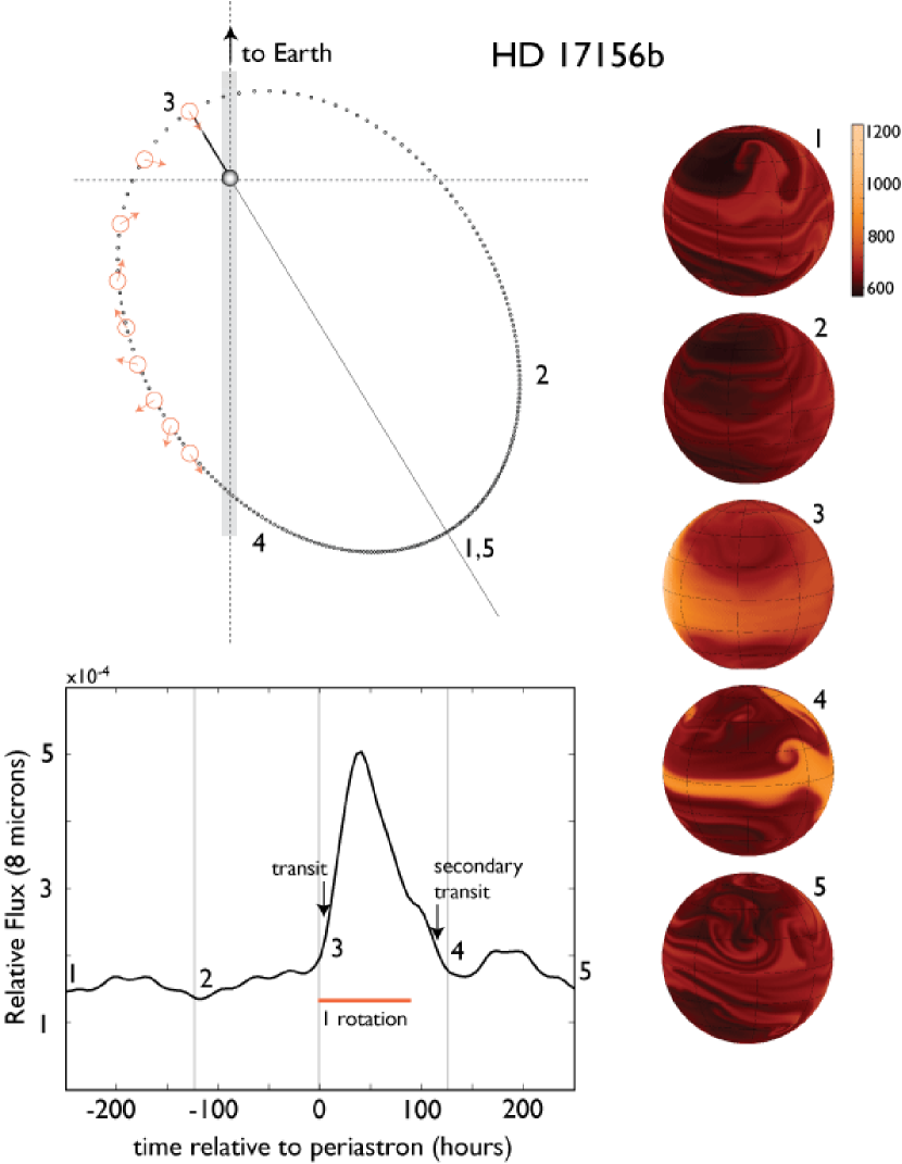
Figure 4.— Upper left hand panel: The orbital geometry of HD 17156b. The small dots show the position of the planet at 2.4 hour intervals throughout the 21.217 day orbit, and show the planet and star drawn to scale ($R_{\star}=1.2\,R_{\odot}$). The locations of the planet at successive time intervals equal to one quarter of an orbit (1-5) are marked. The small orange spheres indicate the 91.3 hour predicted spin frequency of the planet, which is expected to be in pseudo synchronous rotation. Right hand panels: Temperature maps of the planet at locations 1-5, as viewed from the Earth. The temperature scale is mapped to a black body color map that approximates the planet’s visual appearance in its own intrinsic radiation. Lower left panel: Predicted $8~{}{\mu}$m light curve for the planet during the course of one planetary orbit.

The predicted 8$\mu$m flux from the planet is shown in the lower-left corner of the figure, and features a rapid rise from a baseline of $F_{\rm p}/F_{\star}\sim 1.7\times 10^{-4}$ to $F_{\rm p}/F_{\star}\sim 5\times 10^{-4}$ during the $\sim 30$ hour interval following periastron. The magnitude of this rise is comparable with (but slightly less than) that expected for HAT-P-2b and HD 80606b (Langton & Laughlin 2007).

6. Concluding remarks

HD 17156 thus represents a highly interesting system for follow-up studies in the mid infra-red (e.g. using the Spitzer Space Telescope), even if it does not undergo secondary eclipses. Ground-based observations should also be pursued to continue the search for transit timing variations, and hence to constrain the presence of additional bodies in the system, which, given the high orbital eccentricity of the planet HD 17156b, may show interesting dynamical properties and place constraints on planetary formation and evolution scenarios. This discovery represents an important success for the Transitsearch.org project, and highlights the potential rewards of collaboration between distributed networks of amateur astronomers and the professional community.

References

- Adams & Swartztrauber (1999) Adams, J.C. & Swartztrauber, P. N. 1999, Monthly Weather Review, 127, 1872
- Agol et al. (2005) Agol, E., Steffen, J., Sari, R., & Clarkson, W. 2005, MNRAS, 359, 567
- Aigrain et al. (2007) Aigrain, S., Hodgkin, S., Irwin, J., Hebb, L., Irwin, M., Favata, F., Moraux, E. & Pont, F. 2007, MNRAS, 375, 29
- Bakos et al. (2007) Bakos, G. Á., et al. 2007, ApJ, 670, 826
- Barbieri et al. (2007) Barbieri, M., et al. 2007, A&A, 476, L13
- Bodenheimer et al. (2003) Bodenheimer, P., Laughlin, G. & Lin, D. N. C. 2003, ApJ, 592, 555
- Burkert et al. (2005) Burkert, A., Lin, D. N. C., Bodenheimer, P. H., Jones, C. A. & Yorke, H. W. 2005, ApJ, 618, 512
- Burrows et al. (2007) Burrows, A., Hubeny, I., Budaj, J. & Hubbard, W. B. 2007, ApJ, 661, 502
- Charbonneau et al. (2005) Charbonneau, D., et al. 2005, ApJ, 626, 523
- Charbonneau et al. (2007) Charbonneau, D., Brown, T. M., Burrows, A., & Laughlin, G. 2007, in Protostars and Planets V, ed. B. Reipurth, D. Jewitt & K. Keil (Tucson: University of Arizona Press), 701
- Chatterjee et al. (2007) Chatterjee, S., Ford, E. B., & Rasio, F. A. 2007, ApJ, submitted (astro-ph/0703166)
- Cho et al. (2003) Cho, J. Y.-K., Menou, K., Hansen, B. M. S. & Seager, S. 2003, ApJ, 587, L117
- Claret (2000) Claret, A. 2000, A&A, 363, 1081
- Claret (2004) Claret, A. 2000, A&A, 363, 1081
- Collier Cameron et al. (2007) Collier Cameron, A., et al. 2007, MNRAS, 375, 951
- Cooper & Showman (2005) Cooper, C. S. & Showman, A. P. 2005, ApJ, 629, 45
- Cooper & Showman (2006) Cooper, C. S. & Showman, A. P. 2006, ApJ, 649, 1048
- Cowan et al. (2007) Cowan, N. B., Agol, E., & Charbonneau, D. 2007, MNRAS, 379, 641
- Deming et al. (2005) Deming, D., Seager, S., Richardson, L. J., & Harrington, J. 2005, Nature, 434, 740
- Dobbs-Dixon & Lin (2007) Dobbs-Dixon, I. & Lin, D. N. C. 2007, preprint (arXiv:0704.3269)
- Fabrycky & Tremaine (2007) Fabrycky, D., & Tremaine, S. 2007, ApJ, 669, 1298
- Fischer et al. (2007) Fischer, D. A., et al. 2007, ApJ, 669, 1336
- Fortney et al. (2007a) Fortney, J. J., Marley, M. S. & Barnes, J. W. 2007a, ApJ, 659, 1661
- Fortney et al. (2007b) Fortney, J. J., Cooper, C. S., Showman, A. P., Marley, M. S. & Freedman, R. S. 2007b, ApJ, 652, 746
- Gaudi & Winn (2007) Gaudi, B. S., Winn, J. N. 2007, ApJ, 655, 550
- Gillon et al. (2007) Gillon, M., Triaud, A. H. M. J., Mayor, M., Queloz, D., Udry, S., & North, P. 2007, A&A, submitted (arXiv:0712.2073)
- Groth (1986) Groth, E. J. 1986, AJ, 91, 1244
- Harrington et al. (2006) Harrington, J., Hansen, B. M., Luszcz, S. H., Seager, S., Deming, D., Menou, K., Cho, J. Y.-K., & Richardson, L. J. 2006, Science, 314, 623
- Holman & Murray (2005) Holman, M. J., & Murray, N. W. 2005, Science, 307, 1288
- Johns-Krull et al. (2007) Johns-Krull, C. M., et al. 2007, ApJ, in press (arXiv:0712.4283)
- Knutson et al. (2007a) Knutson, H. A., Charbonneau, D., Allen, L. E., Burrows, A., & Megeath, S. T. 2007a, ApJ, in press (arXiv:0709.3984)
- Knutson et al. (2007b) Knutson, H. A., et al. 2007b, Nature, 447, 183
- Loeillet et al. (2007) Loeillet B., et al. 2007, A&A, submitted (arXiv:0707.0679)
- Irwin et al. (2007) Irwin, J., Irwin, M., Aigrain, S., Hodgkin, S., Hebb, L., & Moraux, E. 2007, MNRAS, 375, 1449
- Langton & Laughlin (2007) Langton, J., & Laughlin, G. 2007, ApJ, in press (arXiv:0711.2106)
- Mandel & Agol (2002) Mandel, K., & Agol, E. 2002, ApJ, 580, 171
- Mandushev et al. (2007) Mandushev, G., et al. 2007, ApJ, 667, L195
- Mardling (2007) Mardling, R. A. 2007, MNRAS, 382, 1768
- McLaughlin (1924) McLaughlin, D. B. 1924, ApJ, 60, 22
- Narita et al. (2007) Narita, N., Sato, B., Ohshima, O., & Winn, J. N. 2007, PASJ, submitted (arXiv:0712.2569)
- Press et al. (1992) Press, W. H., Teukolsky, S. A., Vetterling, W. T. & Flannery, B. P. 1992, Numerical Recipes in Fortran 77: The Art of Scientific Computing (Cambridge, UK: Cambridge University Press)
- Rossiter (1924) Rossiter, R. A. 1924, ApJ, 60, 15
- Seagroves et al. (2003) Seagroves, S., Harker, J., Laughlin, G., Lacy, J., & Castellano, T. 2003, PASP, 115, 1355
- Showman & Guillot (2002) Showman, A. P. & Guillot, T. 2002, A&A, 385, 166
- Steffen & Agol (2005) Steffen, J. H., & Agol, E. 2005, MNRAS, 364, L96
- Takeda et al. (2007) Takeda, G., Ford, E. B., Sills, A., Rasio, F., Fischer, D. A., & Valenti, J. A. 2007, ApJS, 168, 297
- Winn (2007) Winn, J. N. 2007, in ASP Conf. Ser. 366, Transiting Extrapolar Planets Workshop, ed. C. Afonso, D. Weldrake, & Th. Henning (San Francisco: ASP), 170
- Winn et al. (2007) Winn, J. N., Holman M. J. & Roussanova A. 2007, ApJ, 657, 1098
- Wu, Murray & Ramsahai (2007) Wu, Y., Murray, N. W., & Ramsahai, J. M. 2007, ApJ, 670, 820