FLCT: A Fast, Efficient Method for Performing Local Correlation Tracking

Abstract

We describe the computational techniques employed in the recently updated Fourier local correlation tracking (FLCT) method. The FLCT code is then evaluated using a series of simple, 2D, known flow patterns that test its accuracy and characterize its errors.

1. Introduction - What is the basic concept behind local correlation tracking (LCT)?

Given a pair of 2D maps (“images”) $I_{1}(x,y,t)$ and $I_{2}(x,y,t2=t1+\delta t)$ of some scalar quantity, with the second image taken slightly later than the first one, what is the 2-d flow field $(v_{x}[x,y],v_{y}[x,y])$ which, when applied to the scalar field in the first image, will most closely resemble the second image? This definition of LCT is not a precise one, and the LCT technique incorporates no physical conservation laws. Schuck (2005) showed that LCT methods are more consistent with an advection equation, rather than a continuity equation. Here, we acknowledge these shortcomings and forge ahead, noting that LCT results must be interpreted carefully.

In Solar Physics, the idea for LCT is generally attributed to November and Simon (1988). In the engineering literature, the problem is known as the “optical flow” problem (see Schuck [2006] and references therein). Here, we present the technique behind the recently upgraded Fourier LCT (FLCT) method, first described in Welsch, Fisher, & Abbett (2004).

2. The Mathematical Approach Used by FLCT

To construct a 2D velocity field that connects two images $I_{1}(x,y)$ and $I_{2}(x,y)$ taken at two different times $t_{1}$ and $t_{2}$, one must start from some given location within both images, compute a velocity vector, and then repeat the calculation while varying that location over all pixel positions. This involves three high-level operations: (1) windowing the input images to isolate the neighborhood around the pixel of interest; (2) computing the correlation function between the two images; and (3) locating the peak of the cross correlation function.

For each pixel at which a velocity is to be computed, a windowing function is used to de-emphasize parts of the image far away from that pixel. FLCT does this localization by multiplying each of the two images by a Gaussian of width $\sigma$, centered at pixel location $(x_{i},y_{j})$. We denote the resulting images as “sub-images” $S_{1}$ and $S_{2}$. The expressions for $S_{1}$ and $S_{2}$ are:

$$S_{1}^{(i,j)}(x,y) = I_{1}(x,y)e^{-[(x-x_{i})^{2}+(y-y_{j})]^{2}/\sigma^{2}}$$

$$S_{2}^{(i,j)}(x,y) = I_{2}(x,y)e^{-[(x-x_{i})^{2}+(y-y_{j})]^{2}/\sigma^{2}}~{}.$$ (1)

The quantity $\sigma$ is a free parameter in FLCT, and its optimal value changes depending on the nature of the image and the size scales present in the velocity field. As discussed in Welsch et al. (2007), one way to choose the optimal $\sigma$ for a given application is to select the $\sigma$ that statistically minimizes the difference between the final image and the advected initial image, $|I_{2}-\delta t(\mathbf{v}\cdot\nabla)I_{1}|.$

For the $(i,j)$th pixel, the cross-correlation function of sub-image 1 with sub-image 2 is defined by

$$C^{i,j}(\delta x,\delta y)=\int\int dx\,dy\,{S^{i,j}_{1}}^{*}(-x,-y)S^{i,j}_{2}(\delta x-x,\delta y-y)~{}.$$ (2)

We want to find, for each pair of sub-images $S_{1}$ and $S_{2}$ centered at position $(x_{i},y_{j})$, the shifts $\delta x$ and $\delta y$ that maximize $C(\delta x,\delta y)$. The amplitude of the shifts, divided by the time $\delta t=t_{2}-t_{1}$ between images 1 and 2 defines the velocity determined by FLCT: $v_{x}=\delta x/\delta t$, and $v_{y}=\delta y/\delta t$.

FLCT uses the convolution theorem to compute $C(\delta x,\delta y)$ using Fourier transforms. If we write ${\cal F}(S_{1})=s_{1}(k_{x},k_{y})$ and, ${\cal F}(S_{2})=s_{2}(k_{x},k_{y}),$ where ${\cal F}$ denotes Fourier transform, then the above equation can be written

$$C^{i,j}(\delta x,\delta y)={\cal F}^{-1}(s_{1}^{*}s_{2})~{},$$ (3)

where ${\cal F}^{-1}$ denotes the inverse Fourier transform. We sometimes find it useful to perform a low-pass Gaussian filter on the functions $s_{1}$ and $s_{2}$ before applying equation (3) if the original images are noisy. Other researchers have used different cross-correlation functions; some calculate the correlation in $x,y$-space, e.g., November and Simon (1988).

Next, we must find the peak of the cross-correlation function. Sub-pixel accuracy is required, as shifts are frequently substantially less than 0.1 pixel. As a practical matter, we find the peak of $f(\delta x,\delta y)=|C^{i,j}(\delta x,\delta y)|$, rather than $C(\delta x,\delta y)$ so that the operation does not involve complex arithmetic. For notational simplicity, we henceforth use $x,y$ for $\delta x,\delta y$ in the following discussion.

Previous versions of FLCT followed November and Simon (1988), and interpolated $f$ around its pixel-accuracy peak onto a finer grid, and took the location of the maximum of the resulting discretely sampled function as the shift. This approach, however, is only as accurate as the resolution of the interpolated grid, and is therefore computationally expensive — many unnecessary interpolations are required to reach the necessary spatial resolution.

Our current version employs a curve-fitting approach to find the peak in $f(x,y)$ that was inspired by that of Chae (2004, private communication; LCT code written in IDL). First, since the images and sub-images are computed at discrete points in space, we identify the pixel coordinates $(x_{m},y_{n})$ of the largest value of $f$, denoting the largest value of $f$ as $f(x_{m},y_{n}).$ Note that $(x_{m},y_{n})$ may not be equal to $(x_{i},y_{j})$, if the location of the peak of $f(x,y)$ has shifted by more than a pixel in $x$ or $y.$ To find the peak to sub-pixel resolution, we then Taylor-expand $f(x,y)$ to 2nd order about the $(x_{m},y_{n})$ location, denoting the expansion as $f_{T}(x,y)$,

$$f_{T}(x,y) \equiv f(x_{m},y_{n})+\frac{\partial f}{\partial x}(x-x_{m})+\frac{\partial f}{\partial y}(y-y_{n})$$

$$+ \frac{\partial^{2}f}{\partial x\partial y}(x-x_{m})(y-y_{n})+\frac{1}{2}\frac{\partial^{2}f}{\partial x^{2}}(x-x_{m})^{2}+\frac{1}{2}\frac{\partial^{2}f}{\partial y^{2}}(y-y_{n})^{2}~{},$$

where the partial derivatives are evaluated at the point $(x_{m},y_{n})$.

At the peak, we require that the $x$ and $y$ partial derivatives of the Taylor expansion $f_{T}(x,y)$ vanish. These conditions result in a pair of linear equations which allow us to solve for the location $(x_{\rm max},y_{\rm max})$ of the peak:

$$x_{\rm max}-x_{m} = \left(\frac{\partial^{2}f}{\partial y^{2}}\frac{\partial f}{\partial x}-\frac{\partial^{2}f}{\partial x\partial y}\frac{\partial f}{\partial y}\right)\left(\left(\frac{\partial^{2}f}{\partial x\partial y}\right)^{2}-\frac{\partial^{2}f}{\partial x^{2}}\frac{\partial^{2}f}{\partial y^{2}}\right)^{-1}$$ (5)

$$y_{\rm max}-y_{n} = \left(\frac{\partial^{2}f}{\partial x^{2}}\frac{\partial f}{\partial y}-\frac{\partial^{2}f}{\partial x\partial y}\frac{\partial f}{\partial x}\right)\left(\left(\frac{\partial^{2}f}{\partial x\partial y}\right)^{2}-\frac{\partial^{2}f}{\partial x^{2}}\frac{\partial^{2}f}{\partial y^{2}}\right)^{-1}~{}.$$ (6)

To evaluate the partial derivatives, we use standard, second-order finite difference expressions, assuming a uniform grid in the sub-images:

$$\frac{\partial f}{\partial x}=(f_{m+1,n}-f_{m-1,n})/2\Delta x \frac{\partial f}{\partial y}=(f_{m,n+1}-f_{m,n-1})/2\Delta y$$ ,

$$\frac{\partial^{2}f}{\partial x^{2}}=(f_{m+1,n}+f_{m-1,n}-2f_{m,n})/\Delta x^{2} \frac{\partial^{2}f}{\partial y^{2}}=(f_{m,n+1}+f_{m,n-1}-2f_{m,n})/\Delta y^{2}$$ ,

$$\frac{\partial^{2}f}{\partial x\partial y}=(f_{m+1,n+1}+f_{m-1,n-1} - f_{m-1,n+1}-f_{m+1,n-1})/4\Delta x\Delta y~{}.$$ (7)

The total shift in $(x,y)$ that corresponds to the peak in $f$ is then given by

$$\delta x=(x_{m}-x_{i})+(x_{\rm max}-x_{m})~{},~{}\delta y=(y_{n}-y_{j})+(y_{\rm max}-y_{n})~{}.$$ (8)

Equations (5) through (8) thus provide a simple and accurate method for finding the peak of the cross- correlation function to sub-pixel resolution.

3. The Computational Approach Used by FLCT

Our method requires two input images, $I_{1}$ and $I_{2}$, recorded at times $t_{1}$ and $t_{2}=t_{1}+dt$. The algorithm then loops over all pixels in $I_{1}$ and $I_{2}$ for which $|I_{1}+I_{2}|/2>I_{\rm thr}$, where $I_{\rm thr}$ is a user-set threshold. For each such pixel, it must:

1. Compute sub-images $S_{1}$ and $S_{2}.$

2. Compute Fourier transforms of $S_{1}$ and $S_{2}$, $s_{1}$ and $s_{2}.$

3. Perform low-pass filters on $s_{1}$, $s_{2}$ if needed.

4. Compute inverse Fourier transform of $s_{1}^{*}s_{2}$. This is $C^{i,j}$.

5. Compute the absolute value of $C^{i,j},|C^{i,j}|$.

6. Compute the shifts $\delta x,\delta y$ that maximize $|C^{i,j}|$.

7. Compute velocities $v_{x}=\delta x/\delta t,v_{y}=\delta y/\delta t.$

The FLCT code, which is currently called flct, was initially written in IDL, but has since been re-written in C for portability and speed. FLCT also uses its own endian-independent binary input format for the images and for the output velocity arrays. FLCT uses the FFTW library (version 3) for computing the Fast-Fourier Transforms needed to compute the cross-correlation functions. We have written IDL procedures which write the two images flct needs into an input file, and which read the flct output file, consisting of two-dimensional, floating point arrays of $v_{x},v_{y}$, and a mask array, $v_{m},$ equal to one in pixels with $|I_{1}+I_{2}|/2>I_{\rm thr}$ and zero elsewhere. These IDL i/o utilities enable flct to be run easily from within an IDL session.

4. Running FLCT

To compile the FLCT code, the only external library needed is the FFTW3 library. To download a copy of the FLCT source code and compilation instructions, along with IDL i/o procedures, go to our web site. Be sure to get the C version (not the IDL version), and get version test_13 or later.

The flct is code invoked from the command-line – either a terminal window on a Unix-like machine, from the command-prompt tool in MS Windows, or from within an IDL session using either a shell escape character or the spawn command. In all cases, the syntax for flct is as follows:

flct infile outfile deltat deltas sigma -t thr -k kr -h -q

Required Arguments:

• infile - Contains 2 images for local correlation tracking. To create infile use the IDL procedure vcimage2out.pro

• outfile - contains output $v_{x},v_{y},v_{m}$ ($x,y$ velocity and mask arrays). Mask array is zero where velocity not computed. To read outfile, use the IDL procedure vcimage3in.pro

• deltat - Amount of time between images.

• deltas - Units of length of the side of a single pixel; velocity is computed in units of deltas/deltat.

• sigma - Sub-images are weighted by Gaussian of width sigma. If sigma is set to 0, only single values of shifts are returned as $v_{x},v_{y}.$ These values correspond to the overall shifts between the two images, and these values can be used to co-register the images if desired.

Optional parameters:

• -t thr - Determines threshold parameter $I_{\rm thr}$. If $|I_{1}+I_{2}|/2<I_{\rm thr}$ in a pixel, then skip calculation of shifts for that pixel. For thr $\in(0,1),$ thr is assumed to be in relative units of the maximum absolute pixel value in $\{|I_{1}|,|I_{2}|\}$. To force thr values between zero and unity to be in absolute units, append an ’a’ to thr. If calculation is skipped for a pixel, then the $v_{m}$ mask array is set to zero at that pixel location. It is otherwise set to 1.

• -k kr - Apply a low-pass filter to the sub-images, with a Gaussian of a characteristic wavenumber that is a factor of $k_{r}$ times the largest possible wave numbers in $x,y$ directions. $k_{r}$ should be positive. (If $kr>>1$, the unfiltered result should be recovered). This option is sometimes useful for datasets that contain noise at high spatial frequencies. Test cases in which MDI Quiet-Sun magnetograms are shifted by 10 milli-pixels frequently result in a factor of two under-estimate by flct of the applied shift. By setting $k_{r}$ to numbers between 0.2 to 0.5, the full applied shifts can be recovered. Experimentation is recommended.

• -h - “hires” mode. Set this flag to use cubic convolution interpolation of the $f(x,y)$ function to re-grid it to higher resolution before finding shift. It is unclear that this interpolation improves accuracy. Currently, this option seldom used, and may be dropped in the future. It has been retained for heritage.

• -q - Flag to suppress printing of all non-error messages.

From within IDL, a simple demonstration of FLCT can be run using the following commands.

IDL$>$ f1=randomu(seed,101,101)
IDL$>$ f2=shift(f1,1,-1)
IDL$>$ vcimage2out,f1,f2,‘testin.dat’
IDL$>$ $flct testin.dat testout.dat 1. 1. 15.
IDL$>$ vcimage3in,vx,vy,vm,‘testout.dat’
IDL$>$ shade_surf,vx
IDL$>$ shade_surf,vy

5. FLCT Speed

How quickly does FLCT run? On a 1.6 GHz Pentium M (laptop processor) running MS Windows XP, the FLCT code flct can process roughly 200 pixels per second for images with over 40,000 pixels (time per pixel is much less than this for smaller images). The code is speeded up dramatically if the -t thr option is used, in which the velocity calculation is skipped if the image values are less than the chosen threshold. There are many avenues available for further speedup of the FLCT code. Very little experimentation has been done with multiple threads thus far. An experimental version of flct written in Fortran, using MPI has been tested on our Linux cluster, grizzly, and the compute speed was found to scale almost perfectly with the number of processors.

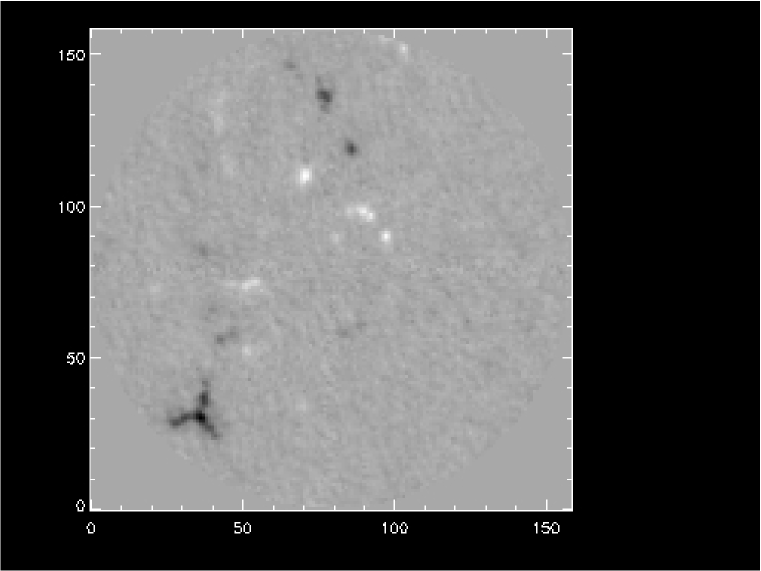
Figure 1.: An MDI magnetogram of the Quiet Sun. By applying known shifts and rotations to such magnetograms, we can test the performance of FLCT.

6. Tests of FLCT

Figure 1 shows an MDI Scherrer et al. (1995) magnetogram of the Quiet Sun. (For a discussion about applying tracking techniques like FLCT to magnetograms, see the paper Welsch and Fisher in this volume.) To test the ability of FLCT to reconstruct rotations, we rotated the image, using cubic-convolution interpolation, by a fixed angle about the center of the image to generate a second image. The applied “velocity field” then corresponds to simple, solid-body rotation, with the speed increasing linearly with radius, $r$, from image center.

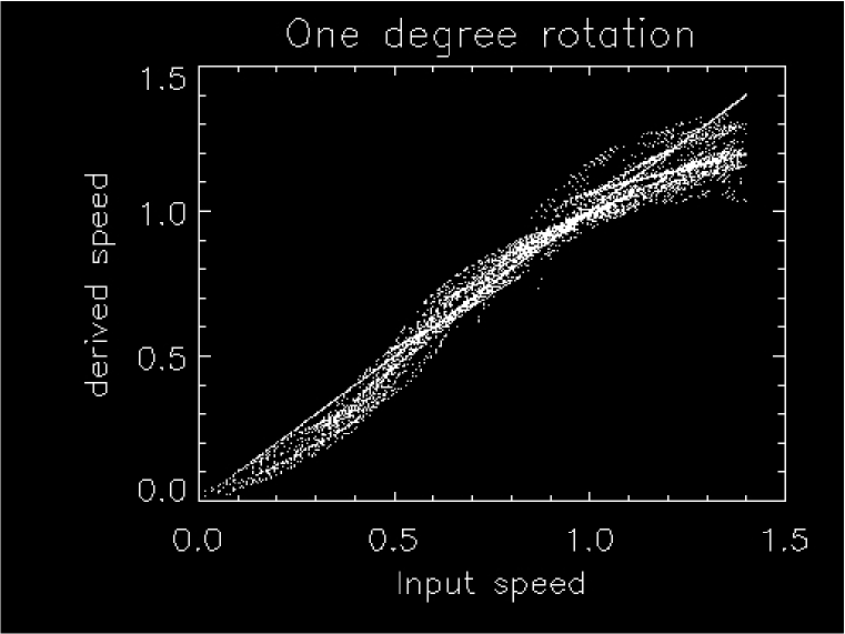
Figure 2.: A scatter plot of derived speeds versus input speeds, for an applied rotation of 1^∘. The straight line shows the applied speed. There is no significant bias in the derived speed.

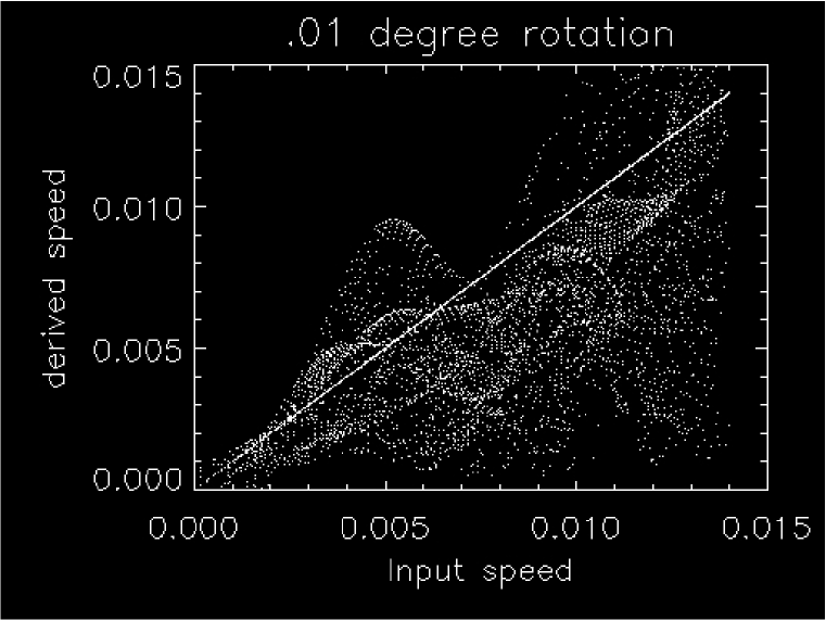
Figure 3.: A scatter plot of derived speeds versus input speeds, for an applied rotation of 0.01^∘. The scatter is significant, and the derived speeds are biased on the low side as compared to the applied speeds.

How well does FLCT recover the applied velocity field? In Figures 2 and 3, we show scatter plots of derived speeds versus input speeds for a rotations of 1^∘ and 0.01^∘, respectively. Units of velocity are in pixel widths per unit time. The straight lines show the applied speed, and the scatter plots show the inverted speeds for all inverted pixels (only points with $|B|>$ 10 G were inverted). $\sigma=$ 15 pixels was assumed. For the 1^∘ rotation, the scatter is typically 0.1-0.2, and there is no significant bias in the derived speed. For the 0.01^∘ rotation, the scatter is significant, and the derived speeds are biased on the low side as compared to the applied speeds. For the 1^∘ rotation, the recovered rotation profile (not shown) accurately reproduces the imposed rotation profile. These and other tests suggest that FLCT can accurately recover shifts $>0.1$ pixels, but smaller shifts can be problematic.

7. Discussion

What is the difference between the new (upgraded) FLCT code, described here, and that originally described in Welsch et al. (2004)? The main difference is in how the location of the peak of the cross-correlation function is determined to sub-pixel resolution. The old version used cubic convolution interpolation to compute the cross-correlation function on a much finer grid (0.1 or 0.02 pixel spacing) and then simply found the location of the largest value within the finer grid. We (and other users) found that this resulted in serious “quantization” errors when the time between images was small enough that shifts were of order 0.1-0.2 pixels or less. The new code uses equations (7) and (8) of this paper to find the location of the peak to sub-pixel resolution. We have found this to be more accurate, and more computationally efficient — and therefore much faster — than the old technique. We strongly recommend that users use the new version and not any of the old versions.

Acknowledgments.

This work was supported by NSF grant ATM-064130, NASA Heliophysics Division through funding from the SR&T and Theory Programs, by NSF-ATM through the SHINE program, and by the DoD MURI grant, ”Understanding Magnetic Eruptions on the Sun and their Interplanetary Consequences”.

References

- November and Simon (1988) November, L. and Simon, G. 1988, ApJ 333, 427.
- Scherrer et al. (1995) Scherrer, P., Bogart, R. S., Bush, R. I., Hoeksema, J. T., Kosovichev, A., Schou, J., Rosenberg, W., Springer, L., Tarbell, T., Title, A., Wolfson, C., Zayer, I., and The MDI Team, 1995, Solar Phys. 162, 129 .
- Schuck (2005) Schuck, P. W. 2005, ApJ 632, L53.
- Schuck (2006) Schuck, P. W. 2006, ApJ646, 1358.
- Welsch et al. (2004) Welsch, B. T., Fisher, G., and Abbett, W. 2004, ApJ 610, 1148.
- Welsch et al. (2007) Welsch, B. T. Abbett, W. P., DeRosa, M. L., Fisher, G. H., Georgoulis, M. K. Kusano, K., Longcope, D. W., Ravindra, B., and Schuck, P. W. 2007, ApJ 670, 1434.111http://solarmuri.ssl.berkeley.edu/welsch/public/manuscripts/Shootout/MaxMil/ms.pdf.