Voter Models on Heterogeneous Networks

Abstract

We study simple interacting particle systems on heterogeneous networks, including the voter model and the invasion process. These are both two-state models in which in an update event an individual changes state to agree with a neighbor. For the voter model, an individual “imports” its state from a randomly-chosen neighbor. Here the average time $T_{N}$ to reach consensus for a network of $N$ nodes with an uncorrelated degree distribution scales as $N\mu_{1}^{2}/\mu_{2}$, where $\mu_{k}$ is the $k^{\rm th}$ moment of the degree distribution. Quick consensus thus arises on networks with broad degree distributions. We also identify the conservation law that characterizes the route by which consensus is reached. Parallel results are derived for the invasion process, in which the state of an agent is “exported” to a random neighbor. We further generalize to biased dynamics in which one state is favored. The probability for a single fitter mutant located at a node of degree $k$ to overspread the population—the fixation probability—is proportional to $k$ for the voter model and to $1/k$ for the invasion process.

I Introduction

Recent studies of statistical physics models on complex networks have elucidated the effect of heterogeneity in link structure on dynamical properties and critical behavior. For scale-free networks, the source of heterogeneity is the broad distribution of node degrees, where node degree is defined as the number of links attached to a node. This dispersity leads, for example, to a vanishing percolation threshold CEAH , allows epidemics to thrive even with a vanishingly small infection rate PV , and causes the Ising model to be ordered at all temperatures DGM .

For many of these models, the dynamics can be understood by accounting for the broadness of the degree distribution within a mean-field description. In this article we show how to implement such an approach for two of the simplest interacting particle systems on heterogeneous networks, namely, the voter model (VM) L ; K92 and its close relative the invasion process (IP) C05 , as well as their generalizations to biased evolution M ; nowak ; WB ; LHN .

For the VM and the IP, each node of an $N$-node network can be in one of two discrete states: $\mathbf{0}$ and $\mathbf{1}$. In a social context, these states represent two possible opinions of the individual at that node. In a biological context, the states represent the phenotype of the individual, with state $\mathbf{0}$ representing resident individuals and $\mathbf{1}$ for mutant individuals. The evolution consists of changing the state of a node at a rate that depends on its local environment. The difference between the VM and IP is in the order in which the “invader” node (whose state is adopted) and the “receiver” node (whose state changes) are chosen. This ordering is immaterial on degree-regular graphs, such as regular lattices, but it plays an essential role on heterogeneous degree networks. Understanding the basic difference between the VM and IP on such graphs is one of the main goals of this work.

We will also study the biased voter model and the biased invasion process in which there is a preference for one of the two states. This generalization describes the evolution of a fitter mutant in an otherwise homogeneous resident population. We will determine the probability for a single fitter mutant to overspread a population with biased VM and biased IP dynamics. Our main result here is that the probability for a single fitter mutant at a node of degree $k$ to overspread a population—the fixation probability—is proportional to $k$ for the VM and to $1/k$ for the IP.

In Sec. II, we define the models of this paper. In Sec. III, we summarize the properties of the VM on the complete graph. We then investigate the VM on heterogeneous networks in Sec. IV, including the complete bipartite graph, the two-clique graph, and general degree-heterogeneous graphs. In Sec. V, we treat the complementary IP. Finally, in Sec. VI, we investigate the biased versions of the VM and the IP and determine the fixation probabilities on general heterogeneous networks.

II Formulation of the Models

II.1 Update Rules

VM evolution consists of the following two steps:

1. pick a random node (a voter);

2. the voter adopts the state of a random neighbor.

In the closely related IP the evolution steps are:

1. pick a random node (an invader);

2. the invader exports its state to a random neighbor.

We also mention an intermediate model, link dynamics (LD), whose evolution steps are:

1. pick a random link;

2. one of the nodes on the link, adopts the state of the other end node.

In these models, the time is incremented by $1/N$ in each update. Thus $N$ updates corresponds to each node being updated once, on average, after which the time increases by 1. Steps (i) and (ii) are then repeated ad infinitum or until the system reaches consensus, an event that is certain to occur in a finite time when the network is finite.

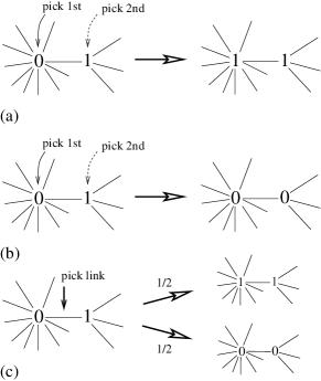
Figure 1: Illustration of the update rules. (a) Voter model (VM): a voter is chosen at random and it adopts the state of random neighbor. (b) Invasion process (IP): a randomly chosen voter exports its state to a neighbor. (c) Link dynamics (LD): an active link is randomly picked and a randomly chosen node at the end of this link is updated.

The interpretation of VM dynamics is that individuals lack any self-confidence. In an update, an individual therefore consults one of its neighbors and adopts the neighbor’s state. On the contrary, in the IP an individual imposes its state to one of its neighbors. Here we can think of the selected individual as replicating, and its offspring invades and replaces the individual at a neighboring node. While the different update details of the three models might appear superficially trivial, we shall show that these differences are fundamental when the dynamics occurs on degree-heterogeneous networks.

In general, such a network may be specified by its adjacency matrix $\mathbf{A}$, with $A_{xy}=1$ if nodes $x$ and $y$ are connected, and $A_{xy}=0$ otherwise. The degree distribution of such a heterogeneous network is specified by

$$n_{k}=\frac{N_{k}}{N}~{},$$ (1)

where $N_{k}$ is the number of nodes of degree $k$ and $N$ is the total number of nodes in the network. The moments of the degree distribution are then

$$\mu_{m}=\frac{1}{N}\sum_{x}k_{x}^{m}=\sum_{k}k^{m}n_{k}\,.$$ (2)

Special cases of relevance for the VM and IP are the average degree $\mu_{1}$, the second moment $\mu_{2}$, and the average inverse degree $\mu_{-1}$. Normalization also fixes the zeroth moment $\mu_{0}=1$.

Let $\eta$ represent the state of the entire network, and define $\eta(x)$, which can take the values 0 or 1, as the state of node $x$. In each update event in the three models, the state of a single node changes from $\mathbf{0}$ to $\mathbf{1}$ or vice versa (Fig. 1). We represent by $\mathbf{\eta}_{x}$ the state of the system that results after changing the state of the node at $x$:

$$\eta_{x}(y)=\begin{cases}\eta(y)&y\neq x\\ 1-\eta(x)&y=x\end{cases}$$ (3)

Transitions are specified by the probability that the state of node $x$ changes, which we term a flip event. For the VM, IP, and LD, the transition probability at node $x$ is

$$\textbf{P}[\eta\to\eta_{x}]=\sum_{y}\frac{A_{xy}}{N\mathcal{Q}}\,[\Phi(x,y)+\Phi(y,x)],$$ (4)

where $\Phi(x,y)\equiv\eta(x)[1-\eta(y)]$, and the quantity

$$A_{xy}\,[\Phi(x,y)+\Phi(y,x)]$$

is non-zero only when nodes $x$ and $y$ are connected (the factor $A_{xy}$) and in opposite states (expression in square brackets), so that an update can actually occur. Finally $\mathcal{Q}$ is

$$\mathcal{Q}\equiv\begin{cases}k_{x}&\textrm{~{}~{}~{}~{}~{}VM},\\ \mu_{1}&\textrm{~{}~{}~{}~{}~{}LD},\\ k_{y}&\textrm{~{}~{}~{}~{}~{}IP}.\end{cases}$$ (5)

For the VM, the factor $(N\mathcal{Q})^{-1}$ in (4) accounts for first choosing node $x$ with probability $1/N$, and then any of its neighbors $y$ with probability $1/\mathcal{Q}=1/k_{x}$. Conversely, in the IP, one first chooses node $y$ (a neighbor of $x$) with probability $1/N$, and then one chooses $x$ with probability $1/\mathcal{Q}=1/k_{y}$. In LD, each link is chosen with the same probability $2/N\mu_{1}$ and then one of the nodes at the end of this link is updated with probability $1/2$, which then leads to $\mathcal{Q}=\mu_{1}$. As we shall discuss, VM, IP, and LD dynamics are distinct for networks with heterogeneous node degrees.

The above models have been defined as discrete-time processes, where one node is chosen in each update step. Alternatively, these models can be formulated as continuous-time processes by increasing the time by a random increment that is chosen from an exponential distribution with mean $1/N$. This stochastic update is equivalent to each update event occurring with unit rate in the three models. For both discrete and continuous time dynamics, the fixation probabilities and the average time to consensus (for long times) are the same. However, there is an essential difference between discrete and continuous time dynamics for biased models that will be discussed in Sec. VI.

II.2 Conservation Laws and Exit Probability

An important aspect of the VM, IP, and LD is that each model has its own dynamically conserved quantity. This conservation law determines the fundamental exit probability $\mathcal{E}_{\mathbf{1}}(\rho)$, namely, the probability that a finite system with an initial density $\rho$ of $\mathbf{1}$s reaches a consensus of all $\mathbf{1}$s. This quantity is also called the fixation probability in the biology literature.

The simplest case is LD, for which the state of the system changes only when an active link—where the nodes at the ends of the link are in opposite states—is chosen. Because the invader and the receiver are assigned randomly, the probability of increasing or decreasing the number of $\mathbf{1}$ nodes (mutants) are the same. The dynamics is thus equivalent to a symmetric random walk on the integers, with absorbing states at $0$ and at $N$ mutants. Because of the symmetry of the random walk, the initial and final densities of nodes in state $\mathbf{1}$ are the same. Consequently, the exit probability is

$$\mathcal{E}_{\mathbf{1}}(\rho)=\rho=\frac{1}{N}\sum_{x}\eta(x)\,.$$ (6)

This result is also valid for the VM and the IP on degree-regular graphs, due to their equivalence to LD when every node has the same degree.

We now extend Eq. (6) to general networks. Consider the average change in $\eta(x)$ at node $x$, $\langle\Delta\eta(x)\rangle$. Here the angle brackets denote the average over all realizations of the update dynamics. This change equals the probability that $\eta(x)$ increases from 0 to 1 minus the probability that $\eta(x)$ decreases from 1 to 0. Hence

$$\langle\Delta\eta(x)\rangle=\left[1-2\eta(x)\right]\mathbf{P}[\eta\rightarrow\eta_{x}]\,.$$ (7)

Substituting the transition probability from Eq. (4), we obtain

$$\langle\Delta\eta(x)\rangle=\sum_{y}\frac{A_{xy}}{N\mathcal{Q}}\left[\eta(y)-\eta(x)\right],$$ (8)

where we use the fact that $\eta(x)^{2}=\eta(x)$. The change in the average density in the entire network, $\langle\Delta\rho\rangle$, is obtained by summing over all nodes $x$ to give

$$\langle\Delta\rho\rangle=\sum_{x}\langle\Delta\eta(x)\rangle=\sum_{x,y}\frac{A_{xy}}{N\mathcal{Q}}\left[\eta(y)-\eta(x)\right]\,.$$ (9)

For LD, and for any of the three models on regular graphs, $\mathcal{Q}$ is constant. Hence the summand in the expression on the right is antisymmetric in $x$ and $y$ and $\langle\Delta\rho\rangle=0$. As a consequence $\langle\rho\rangle$ is conserved, so that the mutant fixation probability equals the initial mutant density $\rho$.

To compute the exit probability on arbitrary networks for general models, we generalize the notion of density by introducing the degree-weighted moments

$$\omega_{m}=\frac{1}{N\mu_{m}}\sum_{x}k_{x}^{m}\eta(x)=\frac{1}{\mu_{m}}\sum_{k}k^{m}n_{k}\rho_{k}\,,$$ (10)

where

$$\rho_{k}\equiv\frac{1}{N_{k}}\sideset{}{{}^{\prime}}{\sum}_{x}\eta(x)\,,$$ (11)

is the density of $\mathbf{1}$s on the subset of nodes of degree $k$. Here the prime on the sum denotes the restriction that all nodes $x$ have fixed degree $k$. Note that $\omega_{0}$ coincides with the density $\rho$. To obtain a conserved quantity, it is clear that the factor $\mathcal{Q}$ in the denominator of the transition rate in (4) must be canceled out. For the VM, we thus consider $\Delta\langle\omega_{1}\rangle$ and repeat the calculation that led to Eq. (9) to obtain

$$\Delta\langle\omega_{1}\rangle=\sum_{x,y}\frac{A_{xy}}{Nk_{x}}k_{x}\left[\eta(y)-\eta(x)\right].$$ (12)

Similarly, the IP, we consider $\Delta\langle\omega_{-1}\rangle$ and obtain

$$\Delta\langle\omega_{-1}\rangle=\sum_{x,y}\frac{A_{xy}}{Nk_{x}k_{y}}\left[\eta(y)-\eta(x)\right].$$ (13)

Because of the $x$-$y$ antisymmetry of the summand in Eqs. (12) and (13), both sums vanish so that the conserved quantity in the three models are:

$$\langle\omega_{1}\rangle$$       VM,

      LD,

      IP.

(14)

We can understand these conservation laws intuitively. For the VM, although nodes are selected uniformly, there are relatively more low-degree nodes that are neighbors of high-degree nodes (see Fig. 1). Thus low-degree nodes change their state more often than high-degree nodes. Weighting each node by its degree compensates this disparity and leads to the conserved quantity $\omega_{1}$. Thus the mean density $\rho$ is not conserved, as first pointed out in Ref. SEM for the VM on heterogeneous graphs. In contrast, For the IP low-degree nodes change their state less often than high degree nodes, and this disparity may be compensated by weighting each node by its inverse degree. This leads to the conserved quantity $\omega_{-1}$.

Figure 2: A star graph.

Since the initial value of the conserved quantity equals its value in the final unanimous state, we obtain, for the exit probability

$$\mathcal{E}_{\mathbf{1}}(\omega_{1})=\omega_{1}$$ VM,

LD & degree regular graphs,

IP,

(15)

An instructive example is the extreme case of a star graph, where $N$ nodes are connected only to a single central hub (Fig. 2). For the VM, if the hub is in state $\mathbf{1}$ and all other nodes are in state $\mathbf{0}$, then Eq. (15) predicts that the probability of reaching $\mathbf{1}$ consensus is 1/2 ! Thus a single individual with a macroscopic number of neighbors largely determines the final state. Conversely, for the IP, this same initial state reaches $\mathbf{1}$ consensus with probability that is $\mathcal{O}(1/N^{2})$. We will discuss this dramatic disparity between VM and IP dynamics in detail in Sec. VI.

III VOTER MODEL ON THE COMPLETE GRAPH

As a preliminary for degree-heterogeneous graphs, we discuss the well-known dynamics of the VM on the complete graph L ; E ; R01 , where each node is connected to every other node. Because the complete graph is degree regular, the VM, IP, and LD are all equivalent and we treat the system in the framework of the VM. Let $\rho(t)$ be the density of voters in state $\mathbf{1}$. In each update event $\rho\to\rho\pm\delta\rho$, with $\delta\rho=1/N$, corresponding to the respective state changes $\mathbf{0}\to\mathbf{1}$ or $\mathbf{1}\to\mathbf{0}$. The probabilities for these events are

$$\begin{split}\mathbf{R}(\rho)\equiv\mathbf{P}[\rho\rightarrow\rho+\delta\rho]=(1-\rho)\rho\\ \mathbf{L}(\rho)\equiv\mathbf{P}[\rho\rightarrow\rho-\delta\rho]=\rho(1-\rho).\end{split}$$ (16)

Here $\mathbf{R}$ and $\mathbf{L}$ denote raising and lowering operators that give the transition probabilities from $\rho$ to $\rho\pm\delta\rho$, respectively.

Let $c(\rho,t)$ be the probability that the density of $\mathbf{1}$’s is $\rho$ at time $t$. After one update event, this density evolves according to

$$c(\rho,t+\delta t) = \mathbf{R}(\rho-\delta\rho)c(\rho-\delta\rho,t)$$ (17)

$$+\mathbf{L}(\rho+\delta\rho)c(\rho+\delta\rho,t)$$

$$+[1-\mathbf{R}(\rho)-\mathbf{L}(\rho)]c(\rho,t).$$

Here $\delta t=1/N$ and the first two terms on the right account for the inflow to the state with density $\rho$ in an update and the last term accounts for outflow. Expanding Eq. (17) to second order in $\delta\rho$ gives the forward Kolmogorov or Fokker-Planck equation VK ,

$$\frac{\partial c(\rho,t)}{\partial t}=\frac{\partial}{\partial\rho}[v(\rho)c(\rho,t)]+\frac{\partial^{2}}{\partial\rho^{2}}[D(\rho)c(\rho,t)],$$ (18)

where

$$v(\rho)\equiv\frac{\delta\rho}{\delta t}[\mathbf{R}(\rho)-\mathbf{L}(\rho)],$$

is the drift term (called the selection term in biology K83 ) that is caused by the bias in the transition probabilities, and

$$D(\rho)\equiv\frac{1}{2}\frac{\delta\rho^{2}}{\delta t}[\mathbf{R}(\rho)+\mathbf{L}(\rho)],$$

is the diffusion term (paradoxically called the random drift term in biology) that quantifies the stochastic noise in the kinetics. On the complete graph, the selection term is zero and the Fokker-Planck equation (18) becomes

$$\frac{\partial c(\rho,t)}{\partial t}=\frac{1}{N}\frac{\partial^{2}}{\partial\rho^{2}}[\rho(1-\rho)c(\rho,t)].$$ (19)

In a similar fashion, the equation for the exit probability with initial density $\rho$ is

$$\mathcal{E}_{\mathbf{1}}(\rho) = \mathbf{R}(\rho)\mathcal{E}_{\mathbf{1}}(\rho\!+\!\delta\rho)+\mathbf{L}(\rho)\mathcal{E}_{\mathbf{1}}(\rho\!-\!\delta\rho)$$ (20)

$$+[1-\mathbf{R}(\rho)-\mathbf{L}(\rho)]\mathcal{E}_{\mathbf{1}}(\rho).$$

This equation expresses $\mathcal{E}_{\mathbf{1}}(\rho)$ as the probability of making a transition to $\rho\pm\delta\rho$ or $\rho$, respectively, times the exit probability from this intermediate point R01 . Expanding Eq. (20) to second order in $\delta\rho$ gives the backward Kolmogorov equation for the exit probability

$$v(\rho)\frac{d\mathcal{E}_{\mathbf{1}}(\rho)}{d\rho}+D(\rho)\frac{d^{2}\mathcal{E}_{\mathbf{1}}(\rho)}{d\rho^{2}}\equiv\mathbf{B}\,\mathcal{E}_{\mathbf{1}}=0,$$ (21)

with $\mathbf{B}$ the generator of the backward Kolmogorov equation. For the boundary conditions $\mathcal{E}_{\mathbf{1}}(\rho\!=\!0)=0$ and $\mathcal{E}_{\mathbf{1}}(\rho\!=\!1)=1$, the solution is simply $\mathcal{E}_{\mathbf{1}}(\rho)=\rho$. This result reproduces Eq. (15) that was obtained by magnetization conservation.

In analogy with Eq. (20), the average time to reach consensus, $T(\rho)$, as a function of the initial density $\rho$, obeys the backward Kolmogorov equation R01

$$T(\rho) = \delta t+\mathbf{R}(\rho)T(\rho\!+\!\delta\rho)+\mathbf{L}(\rho)T(\rho\!-\!\delta\rho)$$ (22)

$$+[1-\mathbf{R}(\rho)-\mathbf{L}(\rho)]T(\rho).$$

This equation expresses the average consensus time as the time for a single step plus the average time to reach consensus after taking this step. The three terms account for the transitions $\rho\rightarrow\rho\pm\delta\rho$ or $\rho\rightarrow\rho$, respectively, and the factor $\delta t$ in each term accounts for the time elapsed in a single update. Expanding Eq. (22) to second order in $\delta\rho$ gives the backward Kolmogorov equation for the average consensus time

$$v(\rho)\frac{dT(\rho)}{d\rho}+D(\rho)\frac{d^{2}T(\rho)}{d\rho^{2}}\equiv\mathbf{B}\,T=-1.$$ (23)

Using the transition probabilities in Eqs. (16) and setting $\delta t=\delta\rho=1/N$, the above equation reduces to

$$\frac{\rho(1-\rho)}{N}\,\frac{d^{2}T(\rho)}{d\rho^{2}}=-1.$$ (24)

For the boundary conditions $T(0)=T(1)=0$, the solution is

$$T(\rho)=N\left[(1-\rho)\ln\frac{1}{1-\rho}+\rho\ln\frac{1}{\rho}\right],$$ (25)

which is symmetric about $\rho=1/2$. Important special cases are $T(1/2)=N\ln 2$, corresponding to starting with equal densities of voters of each opinion, and $T(1/N)\approx\ln N$, corresponding to starting with a single mutant.

In addition to the time to reach either type of consensus, consider the fixation times, namely, the conditional times to reach $\mathbf{1}$ consensus, defined as $T_{\mathbf{1}}(\rho)$, or $\mathbf{0}$ consensus, $T_{\mathbf{0}}(\rho)$, as a function $\rho$. We obtain these times by extending the backward Kolmogorov approach R01 to account for the conditioning on type of consensus. The conditional fixation times satisfy

$$\mathbf{B}\left[\mathcal{E}_{\mathbf{0}}T_{\mathbf{0}}\right]=-\mathcal{E}_{\mathbf{0}}\qquad\mathbf{B}\left[\mathcal{E}_{\mathbf{1}}T_{\mathbf{1}}\right]=-\mathcal{E}_{\mathbf{1}},$$ (26)

with $\mathcal{E}_{\mathbf{0}}=1-\mathcal{E}_{\mathbf{1}}$ and $\mathbf{B}$ is the generator in Eq. (23), subject to absorbing boundaries for both $\mathcal{E}_{\mathbf{0}}T_{\mathbf{0}}$ and $\mathcal{E}_{\mathbf{1}}T_{\mathbf{1}}$. The solution to Eq. (26) is

$$T_{\mathbf{0}}(\rho)=N\frac{\rho}{1-\rho}\ln\frac{1}{\rho}\quad T_{\mathbf{1}}(\rho)=N\frac{1-\rho}{\rho}\ln\frac{1}{1-\rho}~{}.$$ (27)

These fixation times then satisfy the sum rule $\mathcal{E}_{\mathbf{1}}(\rho)T_{\mathbf{1}}(\rho)+\mathcal{E}_{\mathbf{0}}(\rho))T_{\mathbf{0}}(\rho)=T(\rho)$ that reflects the fact that the consensus time is the suitably weighted average of the fixation times. One important limit is the initial state of a single $\mathbf{1}$ mutant, for which the fixation time to all $\mathbf{1}$s is $T_{\mathbf{1}}(1/N)\approx N$. In contrast, the consensus time from this same starting state is much smaller, $T(1/N)\approx\ln N$, because the system can exit via the nearby boundary at $\rho=0$.

IV VOTER MODEL ON COMPLEX NETWORKS

IV.1 The Complete Bipartite Graph

To understand how degree dispersity affects VM dynamics, we first study a simple degree-heterogeneous network, the complete bipartite graph $K_{a,b}$, in which $a+b$ nodes are partitioned into two subgraphs of size $a$ and $b$ (Fig. 3). Each node in the $\mathbf{a}$ subgraph is connected only to all nodes in $\mathbf{b}$, and vice versa. Thus $\mathbf{a}$ nodes all have degree $b$, while $\mathbf{b}$ nodes all have degree $a$.

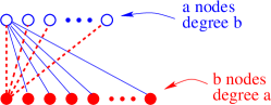
Figure 3: (Color online) The complete bipartite graph $K_{a,b}$.

Consider the voter model on this graph. Let $N_{\mathbf{a},\mathbf{b}}$ be the respective number of voters in state $\mathbf{1}$ on each subgraph and let $\rho_{\mathbf{a}}=N_{\mathbf{a}}/a$, $\rho_{\mathbf{b}}=N_{\mathbf{b}}/b$ be the respective subgraph densities. In an update, these numbers change according to transition probabilities,

$$\begin{split}\mathbf{R}_{\mathbf{a}}\equiv\mathbf{P}[\rho_{\mathbf{a}},\rho_{\mathbf{b}}\rightarrow\rho_{\mathbf{a}}^{+},\rho_{\mathbf{b}}]=\frac{a}{a+b}\,\,\rho_{\mathbf{b}}(1-\rho_{\mathbf{a}}),\\ \mathbf{L}_{\mathbf{a}}\equiv\mathbf{P}[\rho_{\mathbf{a}},\rho_{\mathbf{b}}\rightarrow\rho_{\mathbf{a}}^{-},\rho_{\mathbf{b}}]=\frac{a}{a+b}\,\,\rho_{\mathbf{a}}(1-\rho_{\mathbf{b}}),\end{split}$$ (28)

with $\rho_{\mathbf{a}}^{\pm}=\rho_{\mathbf{a}}\pm a^{-1}$. Here $\mathbf{R}_{\mathbf{a}}$ is the probability to increase the number of $\mathbf{1}$s in subgraph $\mathbf{a}$ by 1, for which we need to first choose a $\mathbf{0}$ in subgraph $\mathbf{a}$ that then interacts with a $\mathbf{1}$ in subgraph $\mathbf{b}$. Similarly, $\mathbf{L}_{\mathbf{a}}$ gives the corresponding the probability for reducing the number of $\mathbf{1}$s in $\mathbf{a}$. Analogous definitions hold for $\mathbf{R}_{\mathbf{b}}$ and $\mathbf{L}_{\mathbf{b}}$ by interchanging $a\leftrightarrow b$.

From these transition probabilities, the rate equations for average subgraph densities are $\frac{d\rho_{\mathbf{a},\mathbf{b}}}{dt}=\rho_{\mathbf{b},\mathbf{a}}-\rho_{\mathbf{a},\mathbf{b}}$ SR , with solution

$$\rho_{\mathbf{a},\mathbf{b}}(t)\!=\!\frac{\rho_{\mathbf{a}}(0)\!+\!\rho_{\mathbf{b}}(0)}{2}\!+\!\frac{[\rho_{\mathbf{a},\mathbf{b}}(0)\!-\!\rho_{\mathbf{b},\mathbf{a}}(0)]e^{-2t}}{2}~{}.$$ (29)

Thus the subgraph densities are driven to the common value $(\rho_{\mathbf{a}}(0)+\rho_{\mathbf{b}}(0))/2$ in a time of the order of one. As a result, the density of $\mathbf{1}$s in the entire graph, which evolves as

$$\frac{d\rho}{dt}=\frac{1}{a+b}\left(a\frac{d\rho_{\mathbf{a}}}{dt}+b\frac{d\rho_{\mathbf{b}}}{dt}\right)=\frac{b-a}{a+b}(\rho_{\mathbf{a}}-\rho_{\mathbf{b}}),$$

becomes conserved in the long-time limit. Thus there is a two-time scale approach to consensus: at early times, there is a non-zero bias that quickly drives the system to equal subgraph densities $\rho_{\mathbf{a}}=\rho_{\mathbf{b}}$; subsequently, diffusive fluctuations drive the eventual approach to consensus.

We can understand this behavior in a more fundamental way by studying the probability that the graph has density of $\mathbf{1}$s equal to $\rho_{\mathbf{a}}$ and $\rho_{\mathbf{b}}$ in each subgraph at time $t$, $c(\rho_{\mathbf{a}},\rho_{\mathbf{b}},t)$. This probability density evolves as

$$c(\rho_{\mathbf{a}},\rho_{\mathbf{b}},t+\delta t)=$$ (30)

$$~{}~{}~{}\mathbf{R}_{\mathbf{a}}(\rho_{\mathbf{a}}^{-},\rho_{\mathbf{b}})\,c(\rho_{\mathbf{a}}^{-},\rho_{\mathbf{b}},t)+\mathbf{L}_{\mathbf{a}}(\rho_{\mathbf{a}}^{+},\rho_{\mathbf{b}})\,c(\rho_{\mathbf{a}}^{+},\rho_{\mathbf{b}},t)$$

$$~{}~{}~{}+\mathbf{R}_{\mathbf{b}}(\rho_{\mathbf{a}},\rho_{\mathbf{b}}^{-})\,c(\rho_{\mathbf{a}},\rho_{\mathbf{b}}^{-},t)+\mathbf{L}_{\mathbf{b}}(\rho_{\mathbf{a}},\rho_{\mathbf{b}}^{+})\,c(\rho_{\mathbf{a}},\rho_{\mathbf{b}}^{+},t)$$

$$~{}~{}~{}~{}~{}+\big{[}1-\mathbf{R}_{\mathbf{a}}(\rho_{\mathbf{a}},\rho_{\mathbf{b}})-\mathbf{L}_{\mathbf{a}}(\rho_{\mathbf{a}},\rho_{\mathbf{b}})$$

$$~{}~{}~{}~{}~{}~{}~{}-\mathbf{R}_{\mathbf{b}}(\rho_{\mathbf{a}},\rho_{\mathbf{b}})-\mathbf{L}_{\mathbf{b}}(\rho_{\mathbf{a}},\rho_{\mathbf{b}})\big{]}\,c(\rho_{\mathbf{a}},\rho_{\mathbf{b}},t).$$

Expanding to second order in $a^{-1}$ and $b^{-1}$ gives the Fokker-Planck equation,

$$\frac{\partial c}{\partial t} \!\!=\!\! -\frac{1}{a\delta t}\frac{\partial}{\partial\rho_{\mathbf{a}}}[(\mathbf{R}_{\mathbf{a}}-\mathbf{L}_{\mathbf{a}})\,c\,]-\frac{1}{b\delta t}\frac{\partial}{\partial\rho_{\mathbf{b}}}[(\mathbf{R}_{\mathbf{b}}-\mathbf{L}_{\mathbf{b}})\,c\,]$$

$$+\frac{1}{2a^{2}\delta t}\frac{\partial^{2}}{\partial\rho_{\mathbf{a}}^{2}}[(\mathbf{R}_{\mathbf{a}}\!+\!\mathbf{L}_{\mathbf{a}})\,c\,]+\frac{1}{2b^{2}\delta t}\frac{\partial^{2}}{\partial\rho_{\mathbf{b}}^{2}}[(\mathbf{R}_{\mathbf{b}}\!+\!\mathbf{L}_{\mathbf{b}})\,c\,].$$

Using $\delta t=1/(a+b)$, we identify the drift velocities for the two subgraph densities as

$$v_{\mathbf{a}} \equiv \frac{a+b}{a}(\mathbf{R}_{\mathbf{a}}-\mathbf{L}_{\mathbf{a}})=\rho_{\mathbf{b}}-\rho_{\mathbf{a}},$$

$$v_{\mathbf{b}} \equiv \frac{a+b}{b}(\mathbf{R}_{\mathbf{b}}-\mathbf{L}_{\mathbf{b}})=\rho_{\mathbf{a}}-\rho_{\mathbf{b}},$$ (32)

that again illustrates the early-time bias in the VM dynamics on the complete bipartite graph. This two-time-scale dynamics is illustrated in Fig. 4, where a bipartite network of size $a=b=10^{5}$ is initialized with $(\rho_{\mathbf{a}}(0),\rho_{\mathbf{b}}(0))=(1,0)$. The dotted curve shows the convective transient that lasts for 3 time steps before the subsequent diffusive approach to the final consensus after 9999.0 steps (solid curve). We define the end of the transient when the trajectory first approaches to within the extent of diffusive fluctuations about the diagonal.

To determine the exit probability, we use the fact that $\omega\equiv(\rho_{\mathbf{a}}+\rho_{\mathbf{b}})/2$ is conserved [see Eq. (15)], so that

$$\mathcal{E}_{\mathbf{1}}(\rho_{\mathbf{a}},\rho_{\mathbf{b}})=\omega(\rho_{\mathbf{a}},\rho_{\mathbf{b}})=\frac{1}{2}(\rho_{\mathbf{a}}+\rho_{\mathbf{b}}).$$ (33)

Strikingly, when one subgraph contains only $\mathbf{0}$s and the other only $\mathbf{1}$s, the probabilities of ending with all $\mathbf{1}$s is 1/2, independent of the subgraph size. To determine the average time $T(\rho_{\mathbf{a}},\rho_{\mathbf{b}})$ to reach consensus—either all $\mathbf{1}$s or all $\mathbf{0}$s—as a function of $\rho_{\mathbf{a}}$ and $\rho_{\mathbf{b}}$, we follow the same steps SR as in Eqs. (22) and (23) to obtain the backward Kolmogorov equation

$$N\delta t \!=\! (\rho_{\mathbf{a}}-\rho_{\mathbf{b}})\left(\frac{\partial T}{\partial\rho_{\mathbf{a}}}-\frac{\partial T}{\partial\rho_{\mathbf{b}}}\right)$$ (34)

$$-\frac{1}{2}(\rho_{\mathbf{a}}\!+\!\rho_{\mathbf{b}}\!-\!2\rho_{\mathbf{a}}\rho_{\mathbf{b}})\left(\frac{1}{a}\frac{\partial^{2}T}{\partial\rho_{\mathbf{a}}^{2}}+\frac{1}{b}\frac{\partial^{2}T}{\partial\rho_{\mathbf{b}}^{2}}\right).~{}~{}~{}~{}~{}~{}$$

The first term on the right accounts for the bias that drives the system to equal subgraph densities while the second term accounts for the diffusion that ultimately drives the system to consensus.

Since the subgraph densities $\rho_{\mathbf{a}}$ and $\rho_{\mathbf{b}}$ asymptotically approach each other and $\omega=(\rho_{\mathbf{a}}+\rho_{\mathbf{b}})/2$, we replace $\rho_{\mathbf{a}}$ and $\rho_{\mathbf{b}}$ by $\omega$ and also $\frac{\partial~{}~{}~{}}{\partial\rho_{\mathbf{a},\mathbf{b}}}$ by $\frac{1}{2}\frac{\partial}{\partial\omega}$ in Eq. (34) to yield

$$\omega(1-\omega)\frac{\partial^{2}T}{\partial\omega^{2}}=-\frac{4ab}{a+b}.$$ (35)

For the boundary conditions $T(0)=T(1)=0$, the solution is [compare with Eq. (25)],

$$T(\omega)=\frac{4ab}{a+b}\left[(1-\omega)\ln\frac{1}{1-\omega}+\omega\ln\frac{1}{\omega}\right].$$ (36)

The consensus time has a similar form to that of the complete graph, but with an effective population size $N_{\mathrm{eff}}\equiv 4ab/(a+b)$. If both components of a bipartite graph have a similar size, $a,b\approx N/2$, then $N_{\rm eff}\approx N$. However, if the two components are disparate, e.g., for $a\sim\mathcal{O}(1)$ and $b\approx N$ then $T\sim\mathcal{O}(1)$ ! Thus one highly-connected node strongly facilitates reaching consensus.

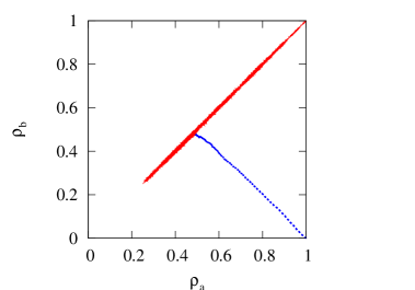
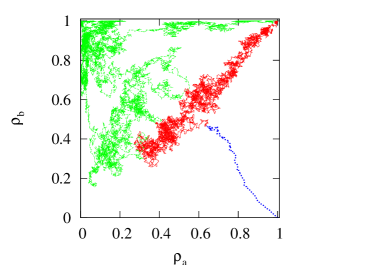
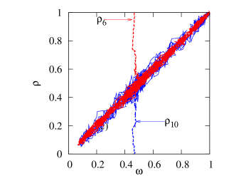
Figure 4: (Color online) Subgraph densities $\rho_{\mathbf{b}}(t)$ versus $\rho_{\mathbf{a}}(t)$ for single realizations of the voter model on (top to bottom): (a) a bipartite graph of $2\times 10^{5}$ nodes; (b) a 2-clique graph of $2\times 10^{4}$ nodes, with $C=1$ (upper trajectory) and $C=100$ (lower trajectory); (c) a Molloy-Reed graph of $2\times 10^{5}$ nodes with degree distribution $n_{k}\sim k^{-2.5}$. For the last example, the densities $\rho_{6}$ and $\rho_{10}$ are shown.

IV.2 The Two-Clique Graph

Another instructive example that reveals the two-time-scale route to consensus is the two-clique graph (Fig. 5). This graph consists of two separate complete graphs of $N$ nodes, $\mathbf{a}$ and $\mathbf{b}$, with each node in one clique also possessing $C$ random cross links to the nodes in the other clique. As we now show, the extent of cross-linking strongly affects how the system reaches consensus.

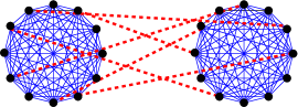
Figure 5: (Color online) The two-clique graph with $N=12$ and $C=1/2$.

For the two-clique network, the respective probabilities that the clique density $\rho_{\mathbf{a}}$ increases or decreases are:

$$\begin{split}&\mathbf{R}_{\mathbf{a}}=\frac{1}{2}(1-\rho_{\mathbf{a}})\left[\frac{N}{N+C}\,\rho_{\mathbf{a}}+\frac{C}{N+C}\,\rho_{\mathbf{b}}\right]\\ &\mathbf{L}_{\mathbf{a}}=\frac{1}{2}\rho_{\mathbf{a}}\left[\frac{N}{N+C}\,(1-\rho_{\mathbf{a}})+\frac{C}{N+C}\,(1-\rho_{\mathbf{b}})\right]\,,\end{split}$$ (37)

with analogous expressions for the rates on clique $\mathbf{b}$. For $\mathbf{R}_{\mathbf{a}}$, the leading factor $\frac{1}{2}$ is the probability of choosing clique $\mathbf{a}$ and $(1-\rho_{\mathbf{a}})$ is the probability of choosing a $\mathbf{0}$ in clique $\mathbf{a}$. The density of $\mathbf{1}s$ in clique $\mathbf{a}$ increases if we choose a $\mathbf{0}$ in clique $\mathbf{a}$ (factor $\frac{N}{N+C}\,\rho_{\mathbf{a}}$) or in clique $\mathbf{b}$ (factor $\frac{C}{N+C}\,\rho_{\mathbf{b}}$). Similar explanations apply for $\mathbf{L}_{\mathbf{a}}$ and for the operators on clique $\mathbf{b}$.

The drift velocity for the density $\rho_{\mathbf{a}}$ is then

$$v_{\mathbf{a}} = \frac{\delta\rho_{\mathbf{a}}}{\delta t}\,(\mathbf{R}_{\mathbf{a}}-\mathbf{L}_{\mathbf{a}})=\frac{C}{N+C}\,\left(\rho_{\mathbf{b}}-\rho_{\mathbf{a}}\right).$$ (38)

When $C$ is $\mathcal{O}(1)$, the drift term is $\mathcal{O}(1/N)$ and is therefore comparable to the diffusive term,

$$D_{\mathbf{a}}=\frac{1}{2}\frac{(\delta\rho_{\mathbf{a}})^{2}}{\delta t}(\mathbf{R}_{\mathbf{a}}+\mathbf{L}_{\mathbf{a}})\propto\frac{(1/N)^{2}}{1/N}\,\frac{N}{N+C}~{},$$ (39)

which remains $\mathcal{O}(1/N)$ for all densities. The clique densities $\rho_{\mathbf{a}}$ and $\rho_{\mathbf{b}}$ thus evolve diffusively and independently until consensus which is reached. This behavior is illustrated in the upper dashed (green online) trajectory of Fig. 4(b) for a single realization of a 2-clique graph with $a=b=10^{4}$ nodes in each clique and with a single crosslink per node for the initial condition $(\rho_{\mathbf{a}}(0),\rho_{\mathbf{b}}(0))=(0,1)$.

Conversely, for $C>\mathcal{O}(1)$ the drift is dominant and the clique densities are driven to a common value that subsequently evolves diffusively along the $\rho_{\mathbf{a}}=\rho_{\mathbf{b}}$ diagonal until consensus is reached as illustrated in the lower trajectory in Fig. 4(b). Shown is the trajectory of a single realization when there are 100 crosslinks per node for the initial condition $(\rho_{\mathbf{a}}(0),\rho_{\mathbf{b}}(0))=(1,0)$. The dotted (blue online) line shows the initial transient of 100 time steps and the solid (red online) line shows the subsequent diffusive approach to consensus at $\rho_{a}=\rho_{b}=1$ in 6437 time steps.

IV.3 Heterogeneous-Degree Networks

We now study the VM on networks with arbitrary degree distributions. Following Eq. (4), the fundamental transition probabilities for increasing and decreasing the density of voters of type $\mathbf{1}$ on nodes of fixed degree $k$ are:

$$\begin{split}\mathbf{R}_{k}[\{\rho_{k}\}]&\!\!\equiv\!\!\mathbf{P}[\rho_{k}\rightarrow\rho_{k}^{+}]=\frac{1}{N}\sideset{}{{}^{\prime}}{\sum}_{x,y}\!\frac{1}{k_{x}}\,A_{xy}\,\Phi(y,x)\\ \mathbf{L}_{k}[\{\rho_{k}\}]&\!\!\equiv\!\!\mathbf{P}[\rho_{k}\rightarrow\rho_{k}^{-}]=\frac{1}{N}\sideset{}{{}^{\prime}}{\sum}_{x,y}\!\frac{1}{k_{x}}\,A_{xy}\,\Phi(x,y),\end{split}$$ (40)

where $\rho_{k}^{\pm}=\rho_{k}\pm N_{k}^{-1}$, and the prime on the sums again denote the restriction to nodes $x$ with fixed degree $k$. In Eq. (40) the densities associated with nodes of degrees $k^{\prime}\neq k$ are unaltered.

We now make the approximation that the degrees of neighboring nodes are uncorrelated, such as in the Molloy-Reed (MR) network MR . Then we may replace the elements of the adjacency matrix elements by their expected values to give

$$A_{xy}\to\langle A_{xy}\rangle=\frac{k_{x}k_{y}}{\mu_{1}N}.$$ (41)

This relation expresses the fact that in the absence of degree correlations, the probability that nodes $x,y$ are connected is proportional to $k_{x}k_{y}$, and the proportionality constant in (41) is determined by using the fact that the average node degree is just $\mu_{1}=\frac{1}{N}\sum_{x,y}A_{xy}$ Substituting the mean-field assumption (41) for $A_{xy}$ in Eq. (40), and using Eqs. (1), (10), and (11), the transition probabilities simplify to

$$\mathbf{R}_{k}=n_{k}\omega(1-\rho_{k}),\qquad\mathbf{L}_{k}=n_{k}\rho_{k}(1-\omega).$$ (42)

Similar to Eq. (22), the recursion formula for the mean consensus time, starting with initial densities $\{\rho_{k}\}$, is

$$T(\{\rho_{k}\}) \!\!=\!\! \delta t+\sum_{k}\mathbf{R}_{k}[\{\rho_{k}\}]T(\rho_{k}^{+})+\sum_{k}\mathbf{L}_{k}[\{\rho_{k}\}]T(\rho_{k}^{-})$$

$$+\Big{[}1-\sum_{k}(\mathbf{R}_{k}[\{\rho_{k}\}]+\mathbf{L}_{k}[\{\rho_{k}\}])\Big{]}T(\{\rho_{k}\}).$$

Expanding (IV.3) to second order in $N_{k}^{-1}$ gives the backward Kolmogorov equation for the consensus time

$$\sum_{k}v_{k}\frac{\partial T}{\partial\rho_{k}}+\sum_{k}D_{k}\frac{\partial^{2}T}{\partial\rho_{k}^{2}}=-1,$$ (44)

with degree-dependent velocity and diffusion coefficients

$$\begin{split}v_{k}&\equiv\frac{\delta\rho_{k}}{\delta t}(\mathbf{R}_{k}-\mathbf{L}_{k})=\omega-\rho_{k},\\ D_{k}&\equiv\frac{(\delta\rho_{k})^{2}}{2\delta t}(\mathbf{R}_{k}+\mathbf{L}_{k})=\frac{\omega+\rho_{k}-2\omega\rho_{k}}{2Nn_{k}}~{}.\end{split}$$ (45)

To simplify the backward equation (44) for the consensus time, we start with the forward Kolmogorov equation for the probability distribution

$$\begin{split}c(\{\rho_{k}\},t\!+\!\delta t)&\!=\!\sum_{k}\mathbf{F}_{k}[\rho_{k}-\delta_{k}]c(\rho_{k}-\delta_{k},t)\\ &\!+\!\sum_{k}\mathbf{B}_{k}[\rho_{k}+\delta_{k}]c(\rho_{k}+\delta_{k},t)\\ &\!+\!\Big{[}1\!-\!\sum_{k}(\mathbf{F}_{k}[\{\rho_{k}\}]\!+\!\mathbf{B}_{k}[\{\rho_{k}\}])\Big{]}c(\{\rho_{k}\},t),\end{split}$$ (46)

and expand to second order to obtain the Fokker-Planck equation

$$\partial_{t}c(\{\rho_{k}\},t)=-\sum_{k}\frac{\partial}{\partial\rho_{k}}v_{k}c+\sum_{k}\frac{\partial^{2}}{\partial\rho_{k}^{2}}D_{k}c.$$ (47)

Now we compute the mean value of the average density $\rho_{k}$ with respect to the above probability distribution to obtain the time dependence

$$\frac{d\langle\rho_{k}\rangle}{dt}=\langle\omega\rangle-\langle\rho_{k}\rangle.$$ (48)

whose solution is, using the conservation of $\omega$,

$$\langle\rho_{k}(t)\rangle=\omega(0)-[\omega(0)-\rho_{k}(0)]e^{-t}.$$ (49)

Thus after a time scale that is of the order of one, all the $\rho_{k}$ approach the common value of the conserved quantity $\omega$ and the drift velocity in (45) vanishes. This dynamics is illustrated in Fig. 4(c) where the trajectory of a single VM realization is shown for a Molloy-Reed network of $2\times 10^{5}$ nodes, with degree distribution $n_{k}\sim k^{-2.5}$. The initial state is $(\rho_{k>\mu_{1}}(0),\rho_{k\leq\mu_{1}}(0))=(0,1)$. Shown are $\rho_{6}(t)$ (degree less than $\mu_{1}=8$) and $\rho_{10}(t)$ (degree greater than $\mu_{1}$) versus $\omega$. The initial transient, which lasts 1.78 time steps, is shown dotted, while consensus occurs after 1742 time steps.

As a result of this rapid approach to the locus $\rho_{k}=\omega$ for each $k$, we may drop the drift term in Eq. (44) and also convert to derivatives with respect to $\omega$ by using

$$\frac{\partial T}{\partial\rho_{k}}=\frac{\partial T}{\partial\omega}\frac{\partial\omega}{\partial\rho_{k}}=\frac{kn_{k}}{\mu_{1}}\frac{\partial T}{\partial\omega},$$

to reduce (44) to

$$\frac{1}{N}\sum_{k}\left(\frac{k^{2}}{\mu_{1}^{2}}n_{k}\right)\omega(1-\omega)\,\,\frac{\partial^{2}T}{\partial\omega^{2}}=-1.$$ (50)

We now define the effective population size by

$$N_{\mathrm{eff}}=N\,\frac{\mu_{1}^{2}}{\mu_{2}},$$ (51)

and comparing Eq. (50) with (24), the consensus time is

$$T_{N}(\omega)=N_{\rm eff}\left[(1-\omega)\ln\frac{1}{1-\omega}+\omega\ln\frac{1}{\omega}\right]~{}.$$ (52)

To compute $N_{\rm eff}$ for a network of $N$ nodes with a power-law degree distribution, $n_{k}\sim k^{-\nu}$, we first determine the maximum degree in the network. We obtain this quantity from the extremal criterion KR02 , $\int_{k_{\textrm{max}}}k^{-\nu}\,dk=\frac{1}{N}$. This condition gives $k_{\textrm{max}}\sim N^{1/(\nu-1)}$, which holds for all $\nu\geq 2$, while for $\nu<2$, the maximum degree remains of the order of $N$. With this upper cutoff, the $m^{\textrm{th}}$ moment of the degree distribution is

$$\mu_{m} \!\!\sim\!\! \int^{k_{\textrm{max}}}k^{m}\,n_{k}\,dk$$ (53)

$$\!\!\sim\!\! \begin{cases}N^{(m\!+\!1\!-\!\nu)/(\nu\!-\!1)}&m\!+\!1\!-\!\nu>0,~{}\nu\geq 2\\ N^{(m\!+\!1\!-\!\nu)}&m\!+\!1\!-\!\nu>0,~{}\nu<2\\ \ln N&m\!+\!1\!-\!\nu=0\\ \mathcal{O}(1)&m\!+\!1\!-\!\nu<0.\end{cases}$$

Using these results, the asymptotic behaviors of $N_{\rm eff}$ and $T_{N}$ are

$$T_{N}\propto N_{\rm eff}\sim\begin{cases}N&\nu>3,\\ N/\ln N&\nu=3,\\ N^{2(\nu-2)/(\nu-1)}&2<\nu<3,\\ (\ln N)^{2}&\nu=2,\\ {\cal O}(1)&\nu<2.\end{cases}$$ (54)

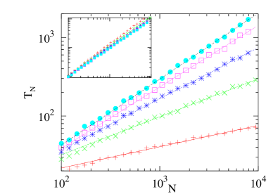
Figure 6: (Color online) Consensus time $T_{N}$ versus $N$ on the Molloy-Reed network with degree distribution $n_{k}=k^{-\nu}$ for $\nu=2.1$ $(+)$, $2.3$ $(\times)$, $2.5$ $(\ast)$, $2.7$ $(\circ)$ and $2.9$ $(\bullet)$. Each data point is based on 100 realizations of the graph and 10 realizations of the voter model on each graph. The lines represent the theoretical prediction of Eq. (54). The inset shows the same data plotted in the scaled form $\mu_{2}T_{N}/\mu_{1}^{2}$ versus $N$.

The main feature of Eq. (54) is that consensus is achieved quickly for the VM, that is, $T_{N}\ll N$ for all $\nu<3$ SR . This consensus time is also much faster than the corresponding behavior on regular lattices in $d$ spatial dimensions L ; K92 : $T_{N}\propto N^{2}$ for $d=1$, $T_{N}\propto N\ln N$ for $d=2$, and $T_{N}\propto N$ for $d>2$. We tested our prediction (54) by simulations of the voter model on both the MR network (Fig. 6) and also a network that is grown by the the redirection algorithm KR01 . This method generates a network with shifted linear attachment rate; that is, the probability of attaching to a node of degree $k$ is given by $k+\lambda$. This growth rule leads to a power-law degree distribution network with tunable exponent $\nu=3+\lambda$. For a network that is generated by the redirection algorithm, the $N$ dependence of $T_{N}$ is essentially the same as that for the MR network (see Fig. 3 of Ref. SR ), and both these numerical results are in good agreement with our theory.

One important feature of the network that is built by the redirection algorithm is that degrees of neighboring nodes are correlated KR01 . In spite of this correlation, the actual values of the consensus times for the MR and the redirection networks are numerically within 15% of each other. Thus evidently degree correlations have a secondary role in determining the consensus time; the broadness of the degree distribution is much more important.

V INVASION PROCESS

We now study the role of degree heterogeneity on IP dynamics, a question that was first studied by Castellano C05 . In analogy with our approach for the voter model, we replace the adjacency matrix elements by their average values, as in Eq. (41), so that the transition probability of Eq. (4) becomes

$$\mathbf{P}[\eta\rightarrow\eta_{x}]=\frac{k_{x}}{\mu_{1}N}[\eta(x)(1-\rho)+(1-\eta(x))\rho].$$ (55)

From this expression, and following exactly the same steps that led to Eq. (42), the transition probabilities for nodes of a fixed given degree are:

$$\mathbf{R}_{k}=n_{k}\frac{k}{\mu_{1}}\rho(1-\rho_{k})\qquad\mathbf{L}_{k}=n_{k}\frac{k}{\mu_{1}}\rho_{k}(1-\rho),$$ (56)

where again $\rho_{k}^{\pm}=\rho\pm N_{k}^{-1}$. The corresponding $k$-dependent drift velocity and diffusion coefficient are then:

$$\begin{split}v_{k}&=\frac{\delta\rho_{k}}{\delta t}(\mathbf{R}_{k}-\mathbf{L}_{k})=\frac{k}{\mu_{1}}(\rho-\rho_{k}),\\ D_{k}&=\frac{(\delta\rho_{k})^{2}}{2\delta t}(\mathbf{R}_{k}+\mathbf{L}_{k})=\frac{k(\rho+\rho_{k}-2\rho\rho_{k})}{2Nn_{k}\mu_{-1}}\end{split}$$ (57)

From the drift velocity, the time dependence of the average density $\rho_{k}$ is determined from

$$\frac{d\langle\rho_{k}\rangle}{dt}=\frac{k}{\mu_{1}}\langle(\rho-\rho_{k})\rangle.$$ (58)

which shows that the densities $\rho_{k}$ again approach the common value $\rho$ after a time scale of $\mathcal{O}(1)$. Once this concurrence happens, we may asymptotically replace $\rho$, and concomitantly all the $\rho_{k}$, by $\omega_{-1}$ in the expressions (57) for $v_{k}$ and $D_{k}$.

With this simplification, we now follow exactly the same steps that led from Eq. (IV.3) to Eq. (52) in the previous section to write backward Kolmogorov equation for the consensus time:

$$\frac{1}{\mu_{1}\mu_{-1}N}\,\,\omega_{-1}\,(1-\omega_{-1})\frac{\partial^{2}T}{\partial\omega_{-1}}=-1.$$ (59)

By comparing with Eqs. (52) and (59), we deduce the average consensus time

$$T_{N}(\omega_{-1})=N_{\rm eff}\left[(1-\omega_{-1})\ln\frac{1}{1-\omega_{-1}}+\omega_{-1}\ln\frac{1}{\omega_{-1}}\right]$$ (60)

with $N_{\rm eff}=N\mu_{1}\mu_{-1}$. For graphs with power-law degree distributions we use the moments written in Eq. (53) to obtain

$$T_{N}\propto N_{\rm eff}\sim\begin{cases}N&\nu>2,\\ N\ln N&\nu=2,\\ N^{3-\nu}&\nu<2.\end{cases}$$ (61)

Thus for all reasonable graphs, those with $\nu>2$, the consensus time for the IP is strictly linear in $N$, in sharp distinction to much faster consensus for the VM.

VI DYNAMICS WITH SELECTION

We now study the VM and IP when the two states $\mathbf{0}$ and $\mathbf{1}$ have different fitnesses. We define resident $\mathbf{0}$s as having fitness $f=1$, and mutant $\mathbf{1}$s having fitness $f=r$, which can, in principle, be either smaller or larger than 1. Our goal is to determine the fixation probability, namely, the probability that a single fitter mutant (i.e., we consider only the case $r>1$) overspreads a population under biased dynamics ARS06 . Such a phenomenon provides a natural description for epidemic propagation AM ; PV01 ; BBPV , the emergence of fads W ; GH ; BHW , social cooperation nowak ; szabo ; SP , or the invasion of an ecological niche by a new species LHN ; nowak ; WB .

We define the update steps in the biased VM as:

1. pick a voter with probability proportional to its inverse fitness ($f^{-1}/N\langle f^{-1}\rangle$);

2. the voter adopts the state of a random neighbor.

Here $\langle f^{-1}\rangle$ is the mean inverse fitness of the population. Thus a weaker voter is more likely to be picked and to be influenced by a neighbor. We can equivalently view the fitness as the inverse of a death rate. Similarly, the evolution steps in the biased IP are:

1. pick an invader with probability proportional to its fitness ($f/N\langle f\rangle$);

2. the invader exports its state to a random neighbor.

We denote by $\langle f\rangle$ the mean fitness of the population that we can equivalently view as the number of offspring produced by an individual. Thus a fitter mutant is more likely to spread its progeny. For both the biased VM and biased IP, we focus on the weak selection limit, with $r=1+s$ and $s\ll 1$.

Thus far, we have studied the VM and IP in discrete time, where the time is incremented by $1/N$ after each update event. For the biased models, it turns out to be simpler to treat continuous-time versions. Thus for the biased VM with continuous dynamics, each individual adopts the state of a random neighbor at a rate proportional to its inverse fitness. Similarly, in the biased IP, each individual exports its progeny to a random neighbor at a rate proportional to its fitness. This rate-based update rule is equivalent to a discrete-time update with the time increment chosen from an exponential distribution, with mean value $1/N\langle f^{-1}\rangle$ for the voter model and $1/N\langle f\rangle$ for the invasion process. The discrete and continuous models are then equivalent except for this overall factor in the time scale.

VI.1 Biased Voter Model

For the biased VM on a general network, the probability of changing the state at node $x$ is, in close analogy with the unbiased case [compare with Eq. (4)],

$$\textbf{P}[\eta\to\eta_{x}]=\sum_{y}\frac{A_{xy}}{Nk_{x}\langle f^{-1}\rangle}\!\!\left[\Phi(y,x)+\frac{1}{r}\,\Phi(x,y)\right],$$ (62)

Following the same approach as in Sec. IV.3, the density $\rho_{k}$ of $\mathbf{1}$s at nodes of degree $k$ increases by $\delta\rho_{k}=1/N_{k}$ with probability $\mathbf{R}_{k}(\eta)$ and decreases by $1/N_{k}$ with probability $\mathbf{L}_{k}(\eta)$ in a single update, where

$$\mathbf{R}_{k}(\eta) = \frac{1}{Nk\langle f^{-1}\rangle}\sideset{}{{}^{\prime}}{\sum}_{xy}A_{xy}\Phi(y,x)$$

$$\mathbf{L}_{k}(\eta) = \frac{1-s}{Nk\langle f^{-1}\rangle}\sideset{}{{}^{\prime}}{\sum}_{xy}A_{xy}\Phi(x,y)$$ (63)

are the respective transition probabilities for ($\mathbf{0}\rightarrow\mathbf{1)}$ and ($\mathbf{1}\rightarrow\mathbf{0})$ in the weak selection limit $s\ll 1$. The primes on the sums again denote the restriction to nodes $x$ of degree $k$. We seek the fixation probability $\mathcal{E}_{\mathbf{1}}$ to the state consisting of all $\mathbf{1}$s as a function of the initial densities of $\mathbf{1}$. This probability obeys the backward Kolmogorov equation $\mathbf{B}\,\mathcal{E}_{\mathbf{1}}=0$ VK ; R01 , subject to the boundary conditions $\mathcal{E}_{\mathbf{1}}(\rho=0)=0$ and $\mathcal{E}_{\mathbf{1}}(\rho=1)=1$. In the diffusion approximation, the generator $\mathbf{B}$ of this equation may be expressed as a sum of the changes in $\rho_{k}$ over all $k$,

$$\mathbf{B}=\frac{1}{\delta t}\sum_{k}\left[\delta\rho_{k}(\mathbf{R}_{k}-\mathbf{L}_{k})\frac{\partial}{\partial\rho_{k}}+\frac{(\delta\rho_{k})^{2}}{2}(\mathbf{R}_{k}+\mathbf{L}_{k})\frac{\partial^{2}}{\partial\rho_{k}^{2}}\right]\,,$$ (64)

with $\delta t=1/N\langle f^{-1}\rangle$.

On degree-regular graphs, the sums in Eq. (63) include all nodes and hence count the total number of active links. For uncorrelated node degrees, the fraction of active links reduces to $\rho(1-\rho)$, and the generator (64) for $s\ll 1$ becomes

$$\mathbf{B}\approx\rho(1-\rho)\left[s\frac{\partial}{\partial\rho}+\frac{1}{N}\frac{\partial^{2}}{\partial\rho^{2}}\right]\,,$$ (65)

The drift and diffusion terms differ by a factor $\mathcal{O}(sN)$, so that selection dominates when the population size $N$ is larger than $\mathcal{O}(1/s)$, while diffusion, or random genetic drift, dominates otherwise. Since the probability of increasing the density of 1s at each update is $r$ times larger than the probability of decreasing this density, the fixation process is the same as the absorption of a uniformly biased random walk in a finite interval. The fixation probability is thus given by the well-known exact formula E

$$\mathcal{E}_{\mathbf{1}}(\rho)=\frac{1-r^{-N\rho}}{1-r^{-N}}.$$ (66)

In the small-selection limit $s\ll 1$, this result approaches the solution of the backward Kolmogorov equation $\mathbf{B}\,\mathcal{E}_{\mathbf{1}}=0$, with generator $\mathbf{B}$ given in (65),

$$\mathcal{E}_{\mathbf{1}}(\rho)=\frac{1-e^{-sN\rho}}{1-e^{-sN}}\equiv\mathcal{F}(sN,\rho)\,,$$ (67)

where for later usage we introduce the notation $\mathcal{F}$ for the fixation probability.

Now we return to degree-heterogeneous networks. Here the conserved quantity for unbiased dynamics is the average degree-weighted density $\omega$ [Eq. (14)]. This conservation law suggests that we study the evolution of $\langle\omega\rangle$ when $r\neq 1$. When node $x$ is updated, $\omega$ changes by

$$\omega(\eta_{x})-\omega(\eta)=k_{x}(1-2\eta(x))/\mu_{1}N,$$ (68)

where $\eta_{x}$ again denotes the state of the system after the update. Thus $\langle\omega\rangle$ evolves as

$$\frac{\partial\langle\omega\rangle}{\partial t} = \frac{1}{\delta t}\sum_{x}[\omega(\eta_{x})-\omega(\eta)]\mathbf{P}[\eta\rightarrow\eta_{x}]$$ (69)

$$= \frac{s}{\mu_{1}N}\sum_{x,y}A_{xy}\Phi(x,y),$$

for $s\ll 1$. Now we use the mean-field assumption (41) for $A_{xy}$ to reduce Eq. (63) to

$$\begin{split}\mathbf{R}_{k}(\eta)&=\frac{1}{\langle f^{-1}\rangle}\,n_{k}\omega(1-\rho_{k}),\\ \mathbf{L}_{k}(\eta)&=\frac{1-s}{\langle f^{-1}\rangle}\,n_{k}\rho_{k}(1-\omega),\end{split}$$ (70)

and Eq. (69) to

$$\frac{\partial\langle\omega\rangle}{\partial t}=s\langle\omega\rangle(1-\langle\omega\rangle),$$ (71)

whose solution is

$$\langle\omega(t)\rangle=\left\{1-[1-\omega(0)^{-1}]e^{-st}\right\}^{-1}\,.$$ (72)

Then the time evolution of $\langle\rho_{k}\rangle$ becomes

$$\frac{\partial\langle\rho_{k}\rangle}{\partial t}\!=\!\frac{\delta\rho_{k}(\mathbf{R}_{k}\!-\!\mathbf{L}_{k})}{\delta t}=\langle\omega\rangle-\langle\rho_{k}\rangle+s(1-\langle\omega\rangle)\langle\rho_{k}\rangle.$$ (73)

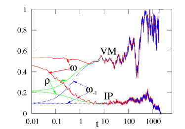
Figure 7: (Color online) Illustration of the two-time-scale dynamics. Moments of the 1 density in the biased VM and the biased IP on a Molloy-Reed network of $10^{4}$ nodes with a power-law degree distribution $n_{k}\sim k^{-\nu}$ and $\nu=2.5$. Nodes with degree larger than the mean degree are initialized to 1 while all other nodes are 0. Here $s=8.13\times 10^{-4}$ for the VM and $s=6.6\times 10^{-5}$ for the IP. These $s$ values were chosen to be $1/N_{\rm eff}$, with $N_{\rm eff}=N\mu_{1}^{2}/\mu_{2}$ for the VM and $N_{\rm eff}=N\mu_{1}\mu_{-1}$ for the IP.

To solve this equation we combine it with Eq. (71) to yield

$$\frac{\partial\langle\omega-\rho_{k}\rangle}{\partial t}=-(1-s)\langle\omega-\rho_{k}\rangle\langle 1-\omega\rangle,$$

with solution

$$\langle\rho_{k}(t)\rangle=\langle\omega(t)\rangle-e^{-t}[\omega(0)-\rho_{k}(0)]\{\omega(0)+[1-\omega(0)]e^{-st}\}\,.$$ (74)

For small selective advantage ($s\ll 1$), this equation involves two distinct time scales. In a time of the order of 1, all the $\rho_{k}$ become equal to $\omega$, the conserved quantity for the unbiased VM. Subsequently, the evolution of $\omega$ itself occurs on a longer time scale of order $s^{-1}\gg 1$ and is driven by the bias (Fig. 7).

We now determine the fixation probability by replacing the $\rho_{k}$ by $\omega$ in the transition probabilities $\mathbf{R}$ and $\mathbf{L}$ in Eqs. (70), and the derivative $\frac{\partial}{\partial\rho_{k}}$ by $\frac{kn_{k}}{\mu_{1}}\frac{\partial}{\partial\omega}$. Then the generator (64) becomes, in the limit $s\ll 1$,

$$\mathbf{B} \approx \omega(1-\omega)\left[s\frac{\partial}{\partial\omega}+\frac{\mu_{2}}{\mu_{1}^{2}N}\frac{\partial^{2}}{\partial\omega^{2}}\right],$$ (75)

which is the same as the generator for degree-regular graphs in Eq. (65) with the population size $N$ replaced by $N_{\rm eff}=N\mu_{1}^{2}/\mu_{2}$. Consequently, the solution to $\mathbf{B}\,\mathcal{E}_{\mathbf{1}}=0$ is simply $\mathcal{E}_{\mathbf{1}}(\omega)=\mathcal{F}(sN_{\rm eff},\omega)$, with $\mathcal{F}$ defined in Eq. (67), that is in excellent agreement with our simulation data (Fig. 8).

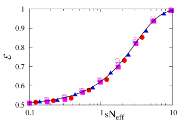
Figure 8: (Color online) Scaling plot of fixation probabilities for VM and IP dynamics for a Molloy-Reed graph with degree distribution $n_{k}\sim k^{-\nu}$ and $\nu=2.5$, with $N=10^{3}$ and $\mu_{1}=8$. The empty symbols correspond to IP dynamics with $s=0.004$ ($\square$), $s=0.008$ ($\circ$) and $s=0.016$ ($\triangle$); the filled symbols correspond to VM dynamics with $s=0.01$, ($\blacksquare$), $s=0.02$ ($\bullet$) and $s=0.08$ ($\blacktriangle$). The smooth curve is the prediction of Eq. (67).

When a single mutant is initially located at a node of degree $k$, then $\omega=k/N\mu_{1}$. Substituting this value into $\mathcal{F}(sN_{\rm eff},\omega)$, we obtain the general result that the fixation probability starting with a single mutant on a node of degree $k$ is proportional to $k$; $\mathcal{E}_{\mathbf{1}}\propto k$ for all $s\ll 1$ (Fig. 9). More precisely, $\mathcal{E}_{\mathbf{1}}\equiv\mathcal{F}(sN_{\rm eff},\omega=k/N\mu_{1})$ has two distinct limiting behaviors:

$$\mathcal{E}_{\mathbf{1}}\to\begin{cases}{\displaystyle\frac{1}{N\mu_{1}}\,\,k}&\quad s\ll 1/N_{\mathrm{eff}};\\ \\ {\displaystyle\frac{s\mu_{1}}{\mu_{2}}\,\,k}&\quad 1/N_{\mathrm{eff}}\ll s\ll 1.\end{cases}$$ (76)

In the $s\ll 1/N_{\mathrm{eff}}$ limit, we recover the results given in Eq. (15) for unbiased evolution. Notice also that the relative influence of selection and random genetic drift is determined by the variable combination $sN_{\textrm{eff}}$. Because $N_{\rm eff}$ can be much less than $N$, diffusion can be important for much larger populations compared to degree-regular graphs.

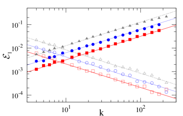
Figure 9: (Color online) Fixation probability of a single mutant initially at a node of degree $k$ on a Molloy-Reed network with $n_{k}\sim k^{-\nu}$ and $\nu=2.5$, with $N=10^{3}$ and $\mu_{1}=8$. The empty symbols correspond to IP dynamics with $s=0.004$ ($\square$), $s=0.008$ ($\circ$) and $s=0.016$ ($\triangle$); the filled symbols correspond to VM dynamics with $s=0.01$, ($\blacksquare$), $s=0.02$ ($\bullet$) and $s=0.08$ ($\blacktriangle$). The solid lines, with slopes $+1$ and $-1$, correspond to the second of Eqs. (76) and (81).

VI.2 Biased Invasion Process

In the complementary biased invasion process, each individual reproduces at a rate proportional to its fitness. Hence the transition probability is

$$\textbf{P}[\eta\to\eta_{x}]=\sum_{y}\frac{A_{xy}}{Nk_{y}\langle f\rangle}\left[r\,\Phi(y,x)+\Phi(x,y)\right]\,.$$ (77)

For degree-uncorrelated graphs and weak selection $s\ll 1$, the transition probabilities for increasing and decreasing $\rho_{k}$ in a single update become

$$\begin{split}\mathbf{R}_{k}(\eta)&=\frac{(1+s)k}{\mu_{1}\langle f\rangle}~{}n_{k}\rho(1-\rho_{k}),\\ \mathbf{L}_{k}(\eta)&=\frac{k}{\mu_{1}\langle f\rangle}~{}n_{k}\rho_{k}(1-\rho).\end{split}$$ (78)

Following the same steps that led to Eq. (73) and using $\delta t=1/N\langle f\rangle$ for continuous-time dynamics, $\rho_{k}$ evolves as

$$\frac{\partial\rho_{k}}{\partial t}=\frac{k}{\mu_{1}}\left[\rho-\rho_{k}+s\rho_{k}(1-\rho)\right],$$ (79)

which implies that all the $\rho_{k}$ rapidly become equal, and, as a consequence, all moments $\omega_{m}$ also become equal. For the unbiased IP, the conserved quantity is $\omega_{-1}$; thus for weak selection, $\omega_{-1}$ is now the most slowly changing quantity, as illustrated in Fig. 7. Hence we replace all $\rho_{k}$ by $\omega_{-1}$, and transform all derivatives with respect to $\rho_{k}$ to derivatives with respect to $\omega_{-1}$ in the generator (64) to obtain

$$\mathbf{B}=\frac{\omega_{-1}(1-\omega_{-1})}{\mu_{1}\mu_{-1}}\left[s\frac{\partial}{\partial\omega_{-1}}+\frac{1}{N}\frac{\partial^{2}}{\partial\omega_{-1}^{2}}\right]$$ (80)

from which, in close analogy with our previous analysis of the VM, the fixation probability is $\mathcal{E}_{\mathbf{1}}(\omega_{-1})=\mathcal{F}(sN,\omega_{-1})$, with $\mathcal{F}$ again defined in Eq. (67).

As a basic corollary, consider the fixation probability when the initial state consists of a single mutant at a node of degree $k$. Substituting $\omega_{-1}=1/kN\mu_{-1}$ into $\mathcal{F}$, we obtain the general results that in the small selection limit $s\ll 1$ the fixation probability is inversely proportional to the node degree, $\mathcal{E}_{1}\sim 1/k$ (fig. 9. The limiting behaviors of the fixation probability are

$$\mathcal{E}_{\mathbf{1}}=\begin{cases}{\displaystyle\frac{1}{N\mu_{-1}}\,\,\frac{1}{k}}&\quad s\ll 1/N;\\ \\ {\displaystyle\frac{s}{\mu_{-1}}\,\,\frac{1}{k}}&\quad 1/N\ll s\ll 1.\end{cases}$$ (81)

In the $s\ll 1/N$ limit we again recover the results in the neutral case (15).

VII DISCUSSION

We developed a unified framework to investigate the dynamics of the voter model (VM), the invasion process (IP), as well as link dynamics (LD) on complex networks. When the relative fitness of the two states, $\mathbf{0}$ and $\mathbf{1}$, are the same, the variable $q$ defined by

$$q\equiv\begin{cases}\omega&\textrm{~{}~{}~{}~{}~{}VM},\\ \rho&\textrm{~{}~{}~{}~{}~{}on regular graphs},\\ \omega_{-1}&\textrm{~{}~{}~{}~{}~{}IP},\end{cases}$$ (82)

is conserved by the dynamics. Because of this conservation law, the exit probability $\mathcal{E}_{\mathbf{1}}$ to $\mathbf{1}$ consensus is simply equal to this conserved variable. This simple result has far-reaching consequences on complex networks, where high-degree nodes can have a disproportionately strong influence.

On complex networks, the evolution of the VM and the IP is governed by two disparate time scales. Initially there is a quick approach to a homogeneous state in which the density of $\mathbf{1}$s on nodes of degree $k$ becomes independent of $k$ for any initial condition. Diffusive fluctuations then drive the system to a final consensus state on a much slower time scale. For a network of $N$ nodes with a power-law degree distribution, $n_{k}\sim k^{-\nu}$, the VM consensus time $T_{N}$ scales slower than linearly with $N$ for all $\nu<3$. This result seems to hold independent of the extent of degree correlations. Thus when the degree distribution is sufficiently broad, high degree nodes facilitate the approach to consensus. In contrast, in the IP, $T_{N}$ scales linearly with $N$ for power-law degree networks for all $\nu>2$.

We also studied the VM and IP with the additional feature of selection, in which individuals in state $\mathbf{1}$ are fitter than those in the $\mathbf{0}$ state. The populations in these two models can be characterized by an effective size

$$N_{\mathrm{eff}}=\begin{cases}{\displaystyle\frac{N\mu_{1}^{2}}{\mu_{2}}}&\quad{\rm VM},\\ \\ N\mu_{1}\mu_{-1}\sim N&\quad{\rm IP\ (\&\ regular\ graphs)}.\end{cases}$$ (83)

The equivalence $N_{\rm eff}\sim N$ applies for the physically accessible case where the mean degree of a graph is finite. From the fixation probabilities given in the previous section, the fundamental parameter for both models is $\alpha\equiv sN_{\mathrm{eff}}$, which is just the Péclet number in the language of biased diffusion. The interesting limit is $s\to 0$ and $N\to\infty$, such that $\alpha$ is constant. Now the general form of the backward Kolmogorov generator is

$$\mathbf{B}=\frac{1}{N_{\mathrm{eff}}}\,\,q(1-q)\left[\alpha\frac{\partial}{\partial q}+\frac{\partial^{2}}{\partial q^{2}}\right]\,.$$ (84)

An important characteristic of the dynamics is the probability that a single $\mathbf{1}$ mutant overspreads an otherwise homogeneous population of $\mathbf{0}$s. This fixation probability satisfies $\mathbf{B}\,\mathcal{E}_{\mathbf{1}}(q)=0$, with solution

$$\mathcal{E}_{\mathbf{1}}(q)=\frac{1-e^{-\alpha q}}{1-e^{-\alpha}}~{},$$ (85)

that depends on the scaling combination $sN{\rm eff}$ and is independent of $s$ and $N_{\mathrm{eff}}$ separately. Another important feature of fixation is its dependence on the degree of the node at which a mutant first appears. For the VM, the probability for a mutant on a node of degree $k$ to fixate is proportional to $k$ [Eq. (76)], while in the complementary IP, the fixation probability is proportional to $1/k$ [Eq. (81)]. The origin of this behavior is simple to understand. In the VM, a well-connected mutant is more likely to be asked its opinion before the mutant queries one of its neighbors. In the IP, a mutant on a high-degree node is more likely to be invaded by a neighbor before the mutant itself can invade. Thus network heterogeneity leads to effective evolutionary heterogeneity.

The above results also allow us to understand the fixation probability for the case where a mutant spontaneously appears at random in the network. For the VM in the selection-dominated regime ($sN_{\rm eff}\gg 1$), averaging Eq. (76) over all nodes gives a fixation probability that is smaller by a factor $\mu_{1}^{2}/\mu_{2}\leq 1$ than that on regular graphs. Thus a heterogeneous graph is an inhospitable environment for a mutant with VM dynamics. The source of this inhospitability is that a spontaneously-appearing mutant is likely to be on a low-degree node, and its state is then quickly erased by interactions with higher-degree nodes. Conversely, for the IP, averaging Eq. (81) over all nodes gives a fixation probability that is independent of the node degree.

Finally, with our general formalism, we can determine the average consensus time from the solution of the backward Kolmogorov equation $\mathbf{B}\,T(q)=-1$. For the unbiased VM and the unbiased IP, this solution has the generic form:

$$T_{N}(q)=N_{\rm eff}\left[(1-q)\ln\frac{1}{1-q}+q\ln\frac{1}{q}\right]~{},$$ (86)

where $q$ is the conserved quantity given in Eq. (82). In the biased case the solution of Eq. (84) can be written as an integral but it is quite cumbersome E . From the form of the generator in Eq. (84), however, it is clear that $T_{N}(q)=N_{\rm eff}\,\tau(q,\alpha)$, and $\tau(q,\alpha)$ is a function that is non singular at $\alpha=0$. Hence, the dependence on effective population size $N_{\mathrm{eff}}$ is not affected by the bias when $\alpha$ is kept constant.

- (1) R. Cohen, K. Erez, D. ben-Avraham, and S. Havlin, Phys. Rev. Lett. 85, 4626 (2000).
- (2) R. Pastor-Satorras and A. Vespignani, Phys. Rev. E 63, 066117 (2001).
- (3) S. N. Dorogovtsev, A. V. Goltsev, and J. F. F. Mendes, Phys. Rev. E 66, 016104 (2002).
- (4) T. M. Liggett, Interacting Particle Systems, (Springer-Verlag, Berlin, 2005).
- (5) P. L. Krapivsky, Phys. Rev. A 45, 1067 (1992).
- (6) C. Castellano, AIP Conference Proceedings 779, 114 2005).
- (7) P. A. P Moran, The Statistical Processes of Evolutionary Theory (Clarendon Press, Oxford, 1962).
- (8) M. A. Nowak, Evolutionary Dynamics, (Harvard Univ. Press, Cambridge MA 2006).
- (9) M. C. Whitlock and N. H. Barton, Genetics 146, 427 (1997).
- (10) E. Lieberman, C. Hauert, and M. A. Nowak, Nature 433, 312 (2005).
- (11) K. Suchecki, V. M. Eguiluz, and M. San Miguel, Europhys. Lett. 69 228 (2005).
- (12) W. Ewens, Mathematical Population Genetics I. Theoretical Introduction, (Springer-Verlag, Berlin, 2004).
- (13) S. Redner, A Guide to First-Passage Processes, (Cambridge University Press, New York, 2001).
- (14) N. G. van Kampen, Stochastic Processes in Physics and Chemistry, ed. (North-Holland, Amsterdam, 1997).
- (15) M. Kimura, The Neutral Theory of Molecular Evolution, (Cambridge University Press, Cambridge, 1983).
- (16) V. Sood and S. Redner, Phys. Rev. Lett. 94, 178701 (2005).
- (17) M. Molloy and B. Reed, Random Structures & Algorithms 6, 161 (1995).
- (18) P. L. Krapivsky and S. Redner, J. Phys. A 35, 9517 (2002).
- (19) P. L. Krapivsky and S. Redner, Phys. Rev. E 63, 066123 (2001).
- (20) T. Antal, S. Redner, and V. Sood, Phys. Rev. Lett. 96, 188104 (2006)
- (21) R. M. Anderson and R. M. May, Infectious Diseases in Humans, (Oxford University Press, Oxford, 1992).
- (22) R. Pastor-Satorras and A. Vespignani, Phys. Rev. Lett. 86, 3200 (2001).
- (23) M. Barthelemy, A. Barrat, R. Pastor-Satorras, and A. Vespignani, Phys. Rev. Lett. 92, 178701 (2004).
- (24) D. J. Watts, Proc. Natl. Acad. Sci. 99, 5766 (2002).
- (25) A. Gronlund and P. Holme, Adv. Complex Systems 8, 261 (2005).
- (26) J. Bendor, B. A. Huberman, and F. Wu, arXiv.org:physics/0509217.
- (27) G. Szabó, G. Fáth, Physics Reports 446, 97 (2007).
- (28) F. C. Santos and J. M. Pacheco, Phys. Rev. Lett. 95, 098104 (2005).