Updating Probabilities: A Complex Agent Based Example

Abstract

It has been shown that one can accommodate data (Bayes) and constraints (MaxEnt) in one method, the method of Maximum (relative) Entropy (ME) (Giffin 2007). In this paper we show a complex agent based example of inference with two different forms of information; moments and data. In this example, several agents each receive partial information about a system in the form of data. In addition, each agent agrees or is informed that there are certain global constraints on the system that are always true. The agents are then asked to make inferences about the entire system. The system becomes more complex as we add agents and allow them to share information. This system can have a geometrical form, such as a crystal structure. The shape may dictate how the agents are able to share information, such as sharing with nearest neighbors. This method can be used to model many systems where the agents or cells have local or partial information but must adhere to some global rules.

1 Introduction

There are many examples of systems where agents respond to both local information as well as global information. Nature yields many such examples where cells react to local stimuli yet carry some global instructions, such as reproduction. The examples get more complex when the cells interact locally or share information. This is the case in physics when one has a lattice or group of many atoms where each is only affected by its nearest neighbor. In all of these cases we would like to infer something about the system or better, what each agent infers about the system. It is this latter case that we will be specifically addressing. The main purpose of this paper is to examine a situation where each agent in a network (of varying degrees of complexity) infers something about the whole system based on limited information. By doing this we hope to attain clues about the system’s emergent properties, such as its dynamics, evolution, etc.

The two preeminent inference methods are the MaxEnt [1] method, which has evolved to a more general method, the method of Maximum (relative) Entropy (ME) [2, 3, 4] and Bayes’ rule. The choice between the two methods has traditionally been dictated by the nature of the information being processed (either constraints or observed data). However, it has been shown that one can accommodate both types of information in one method, ME [5]. In fact, this new ME method can reproduce every aspect of Bayesian and MaxEnt inference and tackle problems that the two methods alone could not address. In this paper we will show how the ME method can be used to infer properties of the system under investigation.

We start by showing a general example of the ME method by inferring a probability with two different forms of information: expected values and data, simultaneously. The solution resembles Bayes’ Rule. In fact, if there are no moment constraints then the method produces Bayes rule exactly. If there is no data, then the MaxEnt solution is produced.

Finally we solve a toy problem where we include global information in the form of a moment constraint or expected value and then introduce local information in the form of data. This will show how the agents infer aspects of the whole system using the same process yet come to different conclusions. Complexity is increased as the number of agents are increased yet the complexity of the process does not grow proportionately. This illustrates the advantages to using the ME method.

2 Simultaneous updating

Our first concern when using the ME method to update from a prior to a posterior distribution is to define the space in which the search for the posterior will be conducted. We wish to infer something about the values of one or several quantities, $\theta\in\Theta$, on the basis of three pieces of information: prior information about $\theta$ (the prior), the known relationship between $x$ and $\theta$ (the model), and the observed values of the data $x\in\mathcal{X}$. Since we are concerned with both $x$ and $\theta$, the relevant space is neither $\mathcal{X}$ nor $\Theta$ but the product $\mathcal{X}\times\Theta$ and our attention must be focused on the joint distribution $P(x,\theta)$. The selected joint posterior $P_{\text{new}}(x,\theta)$ is that which maximizes the entropy,

$$S[P,P_{\text{old}}]=-\int dxd\theta~{}P(x,\theta)\log\frac{P(x,\theta)}{P_{\text{old}}(x,\theta)}~{},$$ (1)

subject to the appropriate constraints. $P_{\text{old}}(x,\theta)$ contains our prior information which we call the joint prior. To be explicit,

$$P_{\text{old}}(x,\theta)=P_{\text{old}}(\theta)P_{\text{old}}(x|\theta)~{},$$ (2)

where $P_{\text{old}}(\theta)$ is the traditional Bayesian prior and $P_{\text{old}}(x|\theta)$ is the likelihood. It is important to note that they both contain prior information. The Bayesian prior is defined as containing prior information. However, the likelihood is not traditionally thought of in terms of prior information. Of course it is reasonable to see it as such because the likelihood represents the model (the relationship between $\theta$ and $x)$ that has already been established. Thus we consider both pieces, the Bayesian prior and the likelihood to be prior information.

The new information is the observed data, $x^{\prime}$, which in the ME framework must be expressed in the form of a constraint on the allowed posteriors. The family of posteriors that reflects the fact that $x$ is now known to be $x^{\prime}$ is such that

$$C_{1}:P(x)=\int d\theta~{}P(x,\theta)=\delta(x-x^{\prime})~{}.$$ (3)

This amounts to an infinite number of constraints: there is one constraint on $P(x,\theta)$ for each value of the variable $x$ and each constraint will require its own Lagrange multiplier $\lambda(x)$. Furthermore, we impose the usual normalization constraint,

$$\int dxd\theta~{}P(x,\theta)=1~{},$$ (4)

and include additional information about $\theta$ in the form of a constraint on the expected value of some function $f(\theta)$,

$$C_{2}:\int dxd\theta\,P(x,\theta)f(\theta)=\left\langle f(\theta)\right\rangle=F~{}.$$ (5)

We emphasize that constraints imposed at the level of the prior need not be satisfied by the posterior. What we do here differs from the standard Bayesian practice in that we require the constraint to be satisfied by the posterior distribution.

Maximize (1) subject to the above constraints,

$$\delta\left\{\begin{array}[]{c}S+\alpha\left[\int dxd\theta P(x,\theta)-1\right]\\ +\beta\left[\int dxd\theta P(x,\theta)f(\theta)-F\right]\\ +\int dx\lambda(x)\left[\int d\theta P(x,\theta)-\delta(x-x{\acute{}})\right]\end{array}\right\}=0~{},$$ (6)

yields the joint posterior,

$$P_{\text{new}}(x,\theta)=P_{\text{old}}(x,\theta)\frac{e^{\lambda(x)+\beta f(\theta)}}{Z}~{},$$ (7)

where $Z$ is determined by using (4),

$$Z=e^{-\alpha+1}=\int dxd\theta e^{\lambda(x)+\beta f(\theta)}P_{\text{old}}(x,\theta)$$ (8)

and the Lagrange multipliers $\lambda(x)$ are determined by using (3)

$$e^{\lambda(x)}=\frac{Z}{\int d\theta e^{\beta f(\theta)}P_{\text{old}}(x,\theta)}\delta(x-x{\acute{}})~{}.$$ (9)

The posterior now becomes

$$P_{\text{new}}(x,\theta)=P_{\text{old}}(x,\theta)\delta(x-x{\acute{}})\frac{e^{\beta f(\theta)}}{\zeta(x,\beta)}~{},$$ (10)

where $\zeta(x,\beta)=\int d\theta e^{\beta f(\theta)}P_{\text{old}}(x,\theta).$

The Lagrange multiplier $\beta$ is determined by first substituting the posterior into (5),

$$\int dxd\theta\left[P_{\text{old}}(x,\theta)\delta(x-x{\acute{}})\frac{e^{\beta f(\theta)}}{\zeta(x,\beta)}\right]f(\theta)=F~{}.$$ (11)

Integrating over $x$ yields,

$$\frac{\int d\theta e^{\beta f(\theta)}P_{\text{old}}(x^{\prime},\theta)f(\theta)}{\zeta(x^{\prime},\beta)}=F~{},$$ (12)

where $\zeta(x,\beta)\rightarrow\zeta(x^{\prime},\beta)=\int d\theta e^{\beta f(\theta)}P_{\text{old}}(x^{\prime},\theta)$. Now $\beta$ can be determined by

$$\frac{\partial\ln\zeta(x^{\prime},\beta)}{\partial\beta}=F~{}.$$ (13)

The final step is to marginalize the posterior, $P_{\text{new}}(x,\theta)$ over $x$ to get our updated probability,

$$P_{\text{new}}(\theta)=P_{\text{old}}(x^{\prime},\theta)\frac{e^{\beta f(\theta)}}{\zeta(x^{\prime},\beta)}$$ (14)

Additionally, this result can be rewritten using the product rule as

$$P_{\text{new}}(\theta)=P_{\text{old}}(\theta)P_{\text{old}}(x^{\prime}|\theta)\frac{e^{\beta f(\theta)}}{\zeta^{\prime}(x^{\prime},\beta)}~{},$$ (15)

where $\zeta^{\prime}(x^{\prime},\beta)=\int d\theta e^{\beta f(\theta)}P_{\text{old}}(\theta)P_{\text{old}}(x^{\prime}|\theta).$ The right side resembles Bayes theorem, where the term $P_{\text{old}}(x^{\prime}|\theta)$ is the standard Bayesian likelihood and $P_{\text{old}}(\theta)$ is the prior. The exponential term is a modification to these two terms. Notice when $\beta=0$ (no moment constraint) we recover Bayes’ rule. For $\beta\neq 0$ Bayes’ rule is modified by a “canonical” exponential factor.

It must be noted that MaxEnt has been traditionally used for obtaining a prior for use in Bayesian statistics. When this is the case, the updating is sequential. This is not the case here where both types of information are processed simultaneously. In the sequential updating case, the multiplier $\beta$ is chosen so that the posterior $P_{\text{new}}$ only satisfies $C_{2}$. In the simultaneous updating case the multiplier $\beta$ is chosen so that the posterior $P_{\text{new}}$ satisfies both $C_{1}$ and $C_{2}$ or $C_{1}\wedge C_{2}$ [5].

3 The agent example

Let us start with a very simple example: There is a class with $3$ students sitting in desks next to each other and one professor. The professor announces that he has a loaded, $3$ sided die and he would like his students to try to discern the probability of getting a $1$, a $2$ or a $3$. He tells them that he has created this die in such a way that on the average, side $1$ is twice as likely to come up as side $3$. Now he rolls the die without showing them the results. He announces that he has rolled the die 10 times. Then he writes down how many times a $1$ came up on a piece of paper and hands it to student A, careful not to let the other students see it. He proceeds to do this for each of the other students, giving student B the results of side $2$ and student C the results of side $3.$ What would each student determine the probabilities of the sides to be? Each needs to determine the probability of getting any particular outcome in one draw ($\theta_{i}$) given the information.

We summarize the information the following way: there are $3$ agents, A, B and C. The die is rolled and the counts of each side are represented by, $m_{1},m_{2}$ and $m_{3}$ respectively with $n$ representing the total count so that $n=\sum\nolimits_{i=1}^{3}m_{i}.$ Additionally, we know that on the average one side, $s_{1}$ is twice as likely to be rolled as $s_{3}.$

The first task is to realize that the correct mathematical model for the probability of getting a particular side where the information that we have is the number of sides counted is a multinomial distribution. The probability of finding $k$ sides in $n$ counts which yields $m_{i}$ instances for the $i^{th}$ side is

$$P_{\text{old}}(m|\theta,n)=P_{\text{old}}(m_{1}\ldots m_{k}|\theta_{1}\ldots\theta_{k},n)=\frac{n!}{m_{1}!\ldots m_{k}!}\theta_{1}^{m_{1}}\ldots\theta_{k}^{m_{k}}~{},$$ (16)

where $m=(m_{1},\ldots,m_{k})$ with $\sum\nolimits_{i=1}^{k}m_{i}=n$, and $\theta=(\theta_{1},\ldots,\theta_{k})$ with $\sum\nolimits_{i=1}^{k}\theta_{i}=1$. The general problem is to infer the parameters $\theta$ on the basis of information about the data, $m^{\prime}.$

Additionally we can include information about the bias of the sides by using the following general constraint,

$$\left\langle f(\theta)\right\rangle=F\quad\text{where}\quad f(\theta)=\sum\nolimits_{i}^{k}f_{i}\theta_{i}~{},$$ (17)

where $f_{i}$ is used to represent the die bias. For our example, on the average, we will find twice the number of $s_{1}$ as compared to $s_{3}$ thus, on the average, the probability of finding one of the sides will be twice that of the other, $\left\langle\theta_{1}\right\rangle=2\left\langle\theta_{3}\right\rangle$. In this case, $f_{1}=1,$ $f_{3}=-2$ and $f_{2}=F=0.$

Next we need to write the data (counts) as a constraint which in general is

$$P(m|n)=\delta(m-m^{\prime})~{},$$ (18)

where $m^{\prime}=\{m_{1}^{\prime},\ldots,m_{k}^{\prime}\}.$ Finally we write the appropriate entropy to use,

$$S[P,P_{\text{old}}]~{}\text{=}-\sum\limits_{m}\int d\theta P(m,\theta|n)\log\frac{P(m,\theta|n)}{P_{\text{old}}(m,\theta|n)}~{},$$ (19)

where

$$\sum\limits_{m}=\sum\limits_{m_{1}\ldots m_{k}=0}^{n}\delta(\sum\nolimits_{i=1}^{k}m_{i}-n)~{},$$ (20)

and

$$\int d\theta=\int d\theta_{1}\ldots d\theta_{k}\,\delta\left(\sum\nolimits_{i=1}^{k}\theta_{i}-1\right)~{},$$ (21)

and where $P_{\text{old}}(m,\theta|n)=P_{\text{old}}(\theta|n)P_{\text{old}}(m|\theta,n).$ The prior $P_{\text{old}}(\theta)$ is not important for our current purpose so for the sake of definiteness we can choose it flat for our example (there are most likely better choices for priors). We then maximize this entropy with respect to $P(m,\theta|n)$ subject to normalization and our constraints which after marginalizing over $m^{\prime}$ yields,

$$P(\theta)=P_{\text{old}}(m^{\prime}|\theta,n)\frac{e^{\beta f(\theta)}}{\zeta}~{},$$ (22)

where

$$\zeta=\int d\theta\,e^{\beta f(\theta)}P_{\text{old}}(m^{\prime}|\theta,n)\quad\text{and}\quad F=\frac{\partial\log\zeta}{\partial\beta}~{}.$$ (23)

Notice that if one has no information relating the sides then $\beta=0.$

For our 3 sided die the probability distribution is

$$P_{\text{e}_{\text{1}}}(\theta_{1},\theta_{2})=\frac{1}{\zeta_{\text{e}}}e^{\beta(3\theta_{1}+2\theta_{2}-2)}\theta_{1}^{m_{1}^{\prime}}\theta_{2}^{m_{2}^{\prime}}(1-\theta_{1}-\theta_{2})^{n-m_{1}^{\prime}-m_{2}^{\prime}}~{}.$$ (24)

However, each student only has the $m^{\prime}$ that corresponds to their side. For example, student A has $m_{1}^{\prime}.$ Therefore student A must marginalize over the unknown information. The result is

$$\sum_{m_{2}=0}^{n-m_{1}}P_{\text{e}_{\text{1}}}(\theta_{1},\theta_{2})=\frac{1}{\zeta_{\text{e}_{\text{1}}}}e^{\beta(3\theta_{1}+2\theta_{2}-2)}\theta_{1}^{m_{1}^{\prime}}(1-\theta_{1})^{n-m_{1}^{\prime}}~{},$$ (25)

where $\zeta_{\text{e}_{\text{1}}}$ is the normalization constant. This is the probability distribution that student A would assign to the die. Since all of the students will follow the same proper inference method (ME), we need only look at one of the student’s solutions. Notice that all students or agents agree on some global information, the bias of the die and the number of total die rolls. However, in general they will determine a different probability distribution that is dependent on the local information, in this case the number of rolls of a particular side.

Now imagine that each student’s desk is at a vertex of an equilateral triangle (so that they are equidistant from each other). They notice that the teacher is looking the other way so they each glance at their neighbor’s paper. Since each of them now have all of the information they should all come up with the same answers.

Next let us create a more complex example by increasing the number of students. We enlarge the class by adding $k$ students with a professor rolling a $k$ sided die that is loaded in some given way. The students are arranged in a lattice structure such as in Figure 1. where there is one student at each of the vertices. Each student that is not on an edge now has six neighbors. Thus if they are allowed to ’look’ at their nearest neighbors, the form of the probability distribution that each student would assign is

$$P_{\text{e}_{\text{2}}}(\theta_{1}...\theta_{k-1})=\frac{1}{\zeta_{\text{e}_{\text{2}}}}e^{\beta f_{k}\left(1-\sum\limits_{i}^{k-1}\theta_{i}\right)}(1-\sum\limits_{i}^{7}\theta_{i})^{n-\sum\limits_{i}^{7}m_{i}}\prod\limits_{i=1}^{7}\theta_{i}^{m_{i}^{\prime}}\prod\limits_{i=1}^{k-1}e^{\beta f_{i}\theta_{i}}~{}.$$ (26)

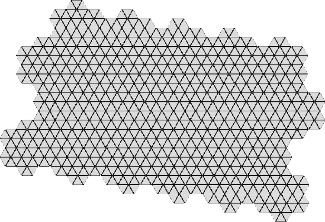
Figure 1: An example structure that relates agents in a system. Here each vertex is an agent.

4 Conclusions

We demonstrated that the ME method can easily lend itself to agent based modeling. Whether the agents are skin cells, atoms in a lattice, banks in a network or students in a classroom, the methodology of ME can be applied in order to model many of these systems. Any system where agents agree on some global information yet react to local information should be able to be modeled with this method. It was further shown that the complexity of the computation can be kept to a minimum since we can marginalize over non-local data.

By determining what each agent ’thinks’ we can predict many properties of the system. An obvious extension of this work would be to apply decision theory concepts to the model so as to not only describe how the agents ’think’ but what they ’choose’ to do as well. This could illustrate how the agents evolve and could illuminate emergent behavior of the system.

By using the ME method we can include additional information which allows us to go beyond what Bayes’ rule and MaxEnt methods alone could do. Therefore, we would like to emphasize that anything one can do with Bayesian or MaxEnt methods, one can now do with ME. Additionally, in ME one now has the ability to apply additional information that Bayesian or MaxEnt methods could not process. Further, any work done with Bayesian techniques can be implemented into the ME method directly through the joint prior.

A currently popular technique is to use entropic concepts on systems. Whether applying entropy in the thermodynamic sense or from the information perspective, ME can help here as well. The realization that the ME entropy $S_{ME}=\log\zeta+\beta F~{}$is of the exact same form as the thermodynamic entropy is of no small consequence. All of the concepts that thermodynamics utilizes can now also be utilized in models using the ME methodology, whether it be energy considerations or equilibrium conditions, etc. In addition, one can get a measure of diversity directly from this method [8]. To see a detailed method for calculating $\zeta,$ see [5]

Acknowledgements: We would like to acknowledge many valuable discussions with A. Caticha.

Bibliography

- [1] E. T. Jaynes, Phys. Rev. 106, 620 and 108, 171 (1957); R. D. Rosenkrantz (ed.), E. T. Jaynes: Papers on Probability, Statistics and Statistical Physics (Reidel, Dordrecht, 1983); E. T. Jaynes, Probability Theory: The Logic of Science (Cambridge University Press, Cambridge, 2003).
- [2] J. E. Shore and R. W. Johnson, IEEE Trans. Inf. Theory IT-26, 26 (1980); IEEE Trans. Inf. Theory IT-27, 26 (1981).
- [3] J. Skilling, “The Axioms of Maximum Entropy”, Maximum-Entropy and Bayesian Methods in Science and Engineering, G. J. Erickson and C. R. Smith (eds.) (Kluwer, Dordrecht, 1988).
- [4] A. Caticha and A. Giffin, “Updating Probabilities”, Bayesian Inference and Maximum Entropy Methods in Science and Engineering, ed. by Ali Mohammad-Djafari (ed.), AIP Conf. Proc. 872, 31 (2006) (http://arxiv.org/abs/physics/0608185).
- [5] A. Giffin and A. Caticha, “Updating Probabilities with Data and Moments”, Bayesian Inference and Maximum Entropy Methods in Science and Engineering, ed. by Kevin Knuth, et all, AIP Conf. Proc. 954, 74 (2007) (http://arxiv.org/abs/0708.1593).
- [6] A. Gelman, et al., Bayesian Data Analysis, 2nd edition (CRC Press, 2004).
- [7] A. Giffin, “Updating Probabilities with Data and Moments: An Econometric Example”, presented at the 3rd Econophysics Colloquium, Ancona, Italy, 2007 (http://arxiv.org/abs/0710.2912).
- [8] A. Giffin, “Infering Diversity: Life after Shannon”, presented at the 7th International Conference on Complex Systems, Boston, 2007 (http://arxiv.org/abs/0709.4079).