The Nature of the Superconducting phase Transitions in Strongly type-II Superconductors in the Pauli Paramagnetic limit

Abstract

Superconducting phase transitions in strongly type-II superconductors in the Pauli paramagnetic limit are considered within the framework of the Gorkov-Ginzburg-Landau approach in the lowest Landau level approximation for both s and d-wave electron pairing. Simple analytical expressions for the quadratic and quartic coefficients in the order parameter expansion of the superconducting free energy are derived without relying on gradient or wavenumber expansions. The existence of a changeover from continuos to discontinuos superconducting phase transitions predicted to occur in the clean limit is shown to depend only on the dimensionality of the underlying electronic band structure. Such a changeover can take place in the quasi 2D regime below a critical value of a 3D-2D crossover parameter.

I Introduction

In recent years a number of unusual superconducting (SC) states have been discovered in different new materials Bennemann04 . Most of these materials are strongly type-II superconductors, possessing highly anisotropic or even quasi-two-dimensional (2D) electronic structures. Of special interest in the present paper are SC materials showing peculiar clean-limit features at high magnetic fields and low temperatures, notably the recently discovered family of heavy-fermion compounds CeRIn₅ (R = Rh, Ir and Co) Petrovic01 , and some of the organic charge transfer salts of the type (BEDT-TTF)₂X Ishiguro90 ,Wosnitza96 .

The heavy-fermion compound CeCoIn₅, for example, which is believed to be an unconventional ( $d$-wave) superconductor Izawa01 similar to the high-Tc cuprates, exhibits the highest Tc ($\sim 2.3$ K) among the Ce-based heavy-Fermion compounds. This material is characterized by exceptionally strong Pauli paramagnetic pair-breaking Clogston62 ,Chandrasekhar62 due to its extremely large electron effective mass and small Fermi velocity, which could lead to discontinuous (first-order) SC phase transitions at sufficiently high magnetic fields Sarma63 ,Maki64 ,Fulde69 .

Recently Bianchi et.al.Bianchi0203 have observed a dramatic changeover of the second-order SC phase transition to a first-order transition in specific heat measurements performed on this material as the magnetic field is increased above some critical values for both parallel and perpendicular field orientations with respect to the easy conducting planes.  Similar effect has been very recently observed by Lortz et.al. Lortz07 in the nearly 2D organic superconductor $\kappa$-(BEDT-TTF)₂Cu(NCS)₂, but only for magnetic field orientation parallel to the superconducting layers, where the orbital (diamagnetic) pair-breaking is completely suppressed. Under these conditions the usual (uniform) SC state is expected to be unstable with respect to formation of a nonuniform SC state, predicted more than 40 years ago by Fulde and Ferrel FF64 , and by Larkin and Ovchinikov LO64 (FFLO). The corresponding SC order parameter is spatially-modulated along the field direction with a characteristic wavenumber, $q$ , whose kinetic energy cost is compensated by the Pauli pair-breaking energy. The critical temperature, $T_{fflo}$, for the appearance of the FFLO phase is found to equal $0.56T_{c}$. At the corresponding tricritical point the normal, the uniform and non-uniform SC phases are all met.

The possibility of a changeover to first-order transitions can be effectively investigated within the Ginzburg-Landau (GL) theory of superconductivity since for the uniform SC phase (i.e. for $q=0$) the coefficient (usually denoted by $\beta$) of the quartic term in the GL expansion changes sign at a temperature $T^{\ast}$, which coincides with $T_{fflo}$ Saint-James69 . The identity of $T^{\ast}$ with $T_{fflo}$ is peculiar to the clean limit of a superconductor with no orbital pair-breaking. In conventional s-wave superconductors electron scattering by non-magnetic impurities shifts $T_{fflo}$ below the critical temperature $T^{\ast}$ Agterberg01 , allowing discontinuous phase transitions at temperatures $T_{fflo}<T\leq T^{\ast}$, since (following Anderson’s theorem) $\beta$ is not influenced by nonmagnetic impurities. In superconductors with unconventional electron pairing, where $\beta$ is strongly influenced by non-magnetic impurity scattering, the situation is reversed, i.e. $T^{\ast}<T_{fflo}$.

The interplay between orbital and spin depairing in a pure $s$-wave isotropic 3D superconductor was first discussed by Gruenberg and Gunthergruenberg66 , who conjectured (i.e. without presenting any result for the coefficient $\beta$ ) that for $T<0.56T_{c}$ the N-SC transition is of the second order whereas at lower field there should be a first-order transition to a uniform SC phase.  Houzet and Buzdinhouzet01 have essentially confirmed this picture by exploiting order-parameter and gradient expansions in the GL theory to find that $T^{\ast}<T_{fflo}$ so that at temperatures $T^{\ast}<T<T_{fflo}$, there are second order transitions to either the LO or FF phase. It should be noted, however, that the orbital effect was treated there by using gradient expansions, which is a valid approximation only at very low magnetic fields.

In contrast to all the works outlined above, Adachi and Ikeda have recently found adachi03 that, in a clean, $d$-wave, 2D (layered) superconductor, the orbital effect always shifts $T_{fflo}$ below $T^{\ast}$. In this work the authors have used order parameter expansion in the Gorkov Green’s function approach to the GL theory up to six order, avoiding the restrictions of gradient expansion by exploiting the lowest Landau level (LLL) approximation for the condensate of Cooper-pairs. Accounting for impurity scattering destroys the FFLO phase and, in contrast to the pure paramagnetic situation, somewhat reduces $T^{\ast}$. The effect of SC thermal fluctuations was found in this work to broaden the discontinuous mean-field transition at $T^{\ast}$ into a crossover. The reliance on (FFLO) wavenumber expansion and on extensive numerical computations in this work has saved formidable analytical efforts, leaving however, interesting questions unanswered. In particular, the origin of the relative shift of $T_{fflo}$ below $T^{\ast}$ by the orbital effect found in this work, in contrast to all the other works, remains unknown.

In the present paper we develop a formalism based on order parameter expansion within the Gorkov theory for a strongly type-II superconductor, with both $s$- and $d_{x^{2}-y^{2}}$-wave electron pairing at high magnetic fields, which is sufficiently simple to yield useful analytical expressions for the SC free energy to any desired order in the expansion. The fundamental interplay between spin induced paramagnetic and orbital diamagnetic effects at an arbitrary magnetic field is studied, within a model of anisotropic electron systems covering the entire 3D-2D crossover range, without relying on gradient or wavenumber expansions. These advantages enable us to shed new light on the yet undecided debate concerning the order of the SC phase transitions in the presence of strong Zeeman spin splitting, and to push our investigation into the unexplored region of very low temperatures, where quantum magnetic oscillations have been shown to be observable in the heavy fermion compounds Settai02 ; Shishido03 .

Specifically, it is found that the relevant parameter controlling the relative position of $T_{fflo}$ with respect to $T^{\ast}$ is the dimensionality of the electronic orbital motion in the crystal lattice, through its influence on the orbital (diamagnetic) pair-breaking effect. For a 3D Fermi surface (isotropic or anisotropic), where the electron motion along the magnetic field direction reduces the cyclotron kinetic energy, the shift of $T^{\ast}$ to low temperatures is larger than that of $T_{fflo}$. In this case the kinetic energy of Cooper-pairs associated with their motion along the field can compensate the spin-splitting effect, and thus leading to an increase of $\beta$ and disappearance of the first-order transition. The corresponding phase diagram is similar to that suggested in Ref. gruenberg66 , where the N-SC transition is of second order, whereas the transition between non-uniform and uniform (along the field) SC states is of first order. In the quasi-2D limit (i.e. for quasi-cylindrical Fermi surfaces) the enhanced orbital pair-breaking shifts $T_{fflo}$ below $T^{\ast}$, in agreement with Adachi and Ikeda adachi03 .

II Order parameter expansion in the presence of spin-splitt Landau levels

Our starting point is an effective BCS-like Hamiltonian with a $d_{x^{2}-y^{2}}$-wave pairing interaction similar to that exploited,e.g. by Agterberg and Yang Agterberg01 . The conventional $s$-wave situation can be similarly worked out and so will not be presented in detail here. The thermodynamical potential (per unit volume) for the corresponding $d$-wave superconductor, as expanded in the order parameter with nonlocal normal electron kernels, may be written as:

$$\Omega=\frac{\Delta_{0}^{2}}{V}+\sum\limits_{m=1}\frac{\left(-1\right)^{m}}{m}\widetilde{\Omega}_{2m}\left\{\Delta\left(\mathbf{R},\mathbf{r}\right)\right\}$$ (1)

where $\widetilde{\Omega}_{2m}\left\{\Delta\left(\mathbf{R},\mathbf{r}\right)\right\}$ is a functional of the SC order parameter, $\Delta\left(\mathbf{R},\mathbf{r}\right)$, having a power-low dependence $\sim|\Delta_{0}|^{2m}$ on the global amplitude, $\Delta_{0}$ , of the order parameter, and $V$ is a BCS coupling constant (given in units of energy$\times$ volume). The corresponding $d$-wave order parameter depends on both the center of mass ($\mathbf{R}$) and relative ($\mathbf{r}$) coordinates of a condensate of electron pairs: $\Delta(\mathbf{R},\mathbf{r})=\Delta(\mathbf{R})\varphi(\mathbf{r})$. It should be determined self-consistently from the corresponding pair-correlation functions. Only stationary solutions are considered, neglecting quantum and thermal fluctuations. In addition the order parameter in the mean field approximation is selected as a hexagonal vortex lattice. Actually this assumption is not very important since the second order term in the order parameter expansion does not depend on the vortex lattice structure whereas the lattice structure dependence of the quartic term is very weak (for reviews see Rasolt-Tesanovic92 ,MRVW92 ).

For the underlying system of normal electrons we assume a simple model of quadratic energy dispersion $\varepsilon\left(k_{x},k_{y},k_{z}\right)=\hbar^{2}\left(k_{x}^{2}+k_{y}^{2}\right)/2m^{\ast}+\hbar^{2}k_{z}^{2}/2m_{z}^{\ast}$ and anisotropic effective mass tensor: $m^{\ast}\leq m_{z}^{\ast}$. A quasi-2D situation is characterized by a sufficiently large anisotropy parameter $\chi_{a}=\sqrt{m_{z}^{\ast}/m^{\ast}}$, corresponding to an elongated Fermi surface with a Fermi momentum $k_{F}$ and Fermi energy $\varepsilon_{F}\equiv\hbar^{2}k_{F}^{2}/2m^{\ast}$, which is truncated by the Brillouin zone (BZ) face at $k_{z,\max}=\pi/d$ , where $d$ is the lattice constant perpendicular to the easy planes. A parameter determining the dimensionality of the Fermi surface may be defined by: $v_{0}=\sqrt{\frac{\varepsilon_{z,\max}}{\varepsilon_{F}}}$ , where $\varepsilon_{z,\max}\equiv\hbar^{2}k_{z,\max}^{2}/2m_{z}^{\ast}$ is the maximal value of the electron energy along the field. Thus, in the 2D limit, $\ k_{z,\max}\ll k_{F}$ , we have $v_{0}\rightarrow 0$ , while the system may be regarded 3D (isotropic or anisotropic ) if $\ k_{z,\max}\simeq k_{F}$ for which the Fermi surface is contained entirely within the first BZ, namely for $v_{0}=1$.

At any order of the expansion, Eq.(1), the nonlocal electronic kernel of the corresponding functional (see e.g. Eqs. (3),(5), and Eqs. (25),(26)) consists of a product of $m=1,2,...$ pairs of normal electron Green’s functions in a constant magnetic field,$\mathbf{H}=H\widehat{z}$ (i.e. perpendicular to the easy conducting layers), which are written in the form:  $G_{\uparrow\downarrow}\left(\mathbf{R}_{1},\mathbf{R}_{2},\omega_{\nu}\right)=G_{0\uparrow\downarrow}\left(\mathbf{R}_{2}-\mathbf{R}_{1},\omega_{\nu}\right)g\left(\mathbf{R}_{1},\mathbf{R}_{2}\right)$, where the gauge factor is given by$\ g\left(\mathbf{R}_{1},\mathbf{R}_{2}\right)=e^{-\frac{i}{2a_{H}}\left[\mathbf{R}_{1}\times\mathbf{R}_{2}\right]\cdot\widehat{z}}$, $a_{H}=\sqrt{c\hbar/eH}$ , and the gauge invariant part can be calculated by the well known expressionBychkov62

$$G_{0\uparrow\downarrow}\left(\mathbf{R}_{2}-\mathbf{R}_{1},\omega_{\nu}\right)=\frac{1}{2\pi a_{H}^{2}}\int\frac{dk_{z}}{2\pi}e^{ik_{z}(Z_{2}-Z_{1})}\sum_{n}\dfrac{e^{-\rho^{2}/4}L_{n}(\rho^{2}/2)}{\mu-\varepsilon_{nk_{z}\uparrow\downarrow}+i\hbar\omega_{\nu}+i\mathrm{sign}\left(\omega_{\nu}\right)\hbar\Gamma}$$ (2)

Here $\omega_{\nu}=\pi k_{B}T\left(2\nu+1\right)/\hbar$ with $\nu=0,\pm 1,...$ is Matzubara frequency, $\varepsilon_{nk_{z}\uparrow}=\hbar\omega_{c}\left(n+1/2+x^{2}-g/2\right)$ ,  $\varepsilon_{nk_{z}\downarrow}=\omega_{c}\left(n+1/2+x^{2}+g/2\right)$, the spin-split normal electron energy levels, $\omega_{c}=eH/m^{\ast}$-the in-plane electronic cyclotron frequency, $x^{2}=\xi^{2}k_{z}^{2}\equiv\frac{k_{z}^{2}}{2m_{z}^{\ast}\omega_{c}}$is a dimensionless longitudinal (parallel to the magnetic field) kinetic energy, $\omega_{c}g\equiv eH/m_{0}$, is the Zeeman spin splitting energy, $\Gamma$- the impurity scattering relaxation rate, and $\mu=\hbar\omega_{c}\left(n_{F}+1/2\right)\approx\varepsilon_{F}=\hbar^{2}k_{F}^{2}/2m^{\ast}$ is the chemical potential. The spatial variables are dimensionless in-plane (perpendicular to the magnetic field) coordinates, $\mathbf{\rho}=\frac{\mathbf{R}_{2\bot}-\mathbf{R}_{1\bot}}{a_{H}}$, and longitudinal coordinates:$\ Z_{1}=\mathbf{R}_{1}\cdot\widehat{z}$ , and $Z_{2}=\mathbf{R}_{2}\cdot\widehat{z}$.

II.1 The quadratic term

In the expansion, Eq.(1), the second order term, which describes the SC condensation energy of spin-singlet electron-pairs, propagating from initial ($i=1$) to final ($i=2$) coordinates $\mathbf{R}_{i}\pm\frac{\mathbf{r}_{i}}{2}$, is given by:

$$\Omega_{2}=\frac{\Delta_{0}^{2}}{V}-\frac{1}{\mathcal{V}_{0}}\int d^{3}\mathbf{R}_{1}d^{3}\mathbf{R}_{2}\tilde{\Gamma}_{2}\left(\mathbf{R}_{1},\mathbf{R}_{2}\right)\tilde{K}_{2}\left(\mathbf{R}_{1},\mathbf{R}_{2}\right)\equiv\frac{\Delta_{0}^{2}}{V}-A_{0}\Delta_{0}^{2}$$ (3)

where $\mathcal{V}_{0}=SL_{z}$ is the volume of the system. The vertex part, $\tilde{\Gamma}_{2},$ is a product of two order parameters multiplied by the gauge factors, $g\left(\mathbf{R}_{2},\mathbf{R}_{1}\right)$, which are functions of the center of mass coordinates only, due to cacellation by the corresponding phase factors of the order parameters, namely:

$$\tilde{\Gamma}_{2}\left(\mathbf{R}_{1},\mathbf{R}_{2}\right)=g^{\ast}\left(\mathbf{R}_{1},\mathbf{R}_{2}\right)g\left(\mathbf{R}_{2},\mathbf{R}_{1}\right)\Delta\left(\mathbf{R}_{1}\right)\Delta^{\star}\left(\mathbf{R}_{2}\right)$$ (4)

The kernel $\tilde{K}_{2}$ is a product of two translational invariant Green’s functions, convoluted with the corresponding factors of the order parameters, which depend only on the relative pair coordinates, namely:

$$\tilde{K}_{2}\left(\mathbf{R}_{1},\mathbf{R}_{2}\right)=k_{B}T\sum_{\nu}\int d^{3}\mathbf{r}_{1}d^{3}\mathbf{r}_{2}\varphi\left(\mathbf{r}_{1}\right)\varphi^{\ast}\left(\mathbf{r}_{2}\right)$$ (5)

$$\times G_{0\uparrow}^{\ast}\left(\mathbf{R}_{2}-\mathbf{R}_{1}+\frac{\mathbf{r}_{2}-\mathbf{r}_{1}}{2},\omega_{\nu}\right)G_{0\downarrow}\left(\mathbf{R}_{1}-\mathbf{R}_{2}+\frac{\mathbf{r}_{2}-\mathbf{r}_{1}}{2},\omega_{\nu}\right)$$

The factor of the order parameter which depends on the pair center of mass coordinates is written asRMP01 :

$$\Delta\left(\mathbf{R}\right)=c(Z)\sum\limits_{n}e^{i\pi n^{2}/2}\phi_{n}\left(\mathbf{R}_{\bot}\right);\ \ \ \ \ \ \ \ \phi_{n}\left(\mathbf{R}_{\bot}\right)=e^{i\frac{2\pi n}{a_{x}}X-\left(Y-\frac{\pi n}{a_{x}}\right)^{2}};\ \ \ \ \ \ a_{x}=$$ (6)

where $c(Z)=c_{0}e^{iqZ}$ is the Fulde-Ferrell modulation factor. Exploiting the fact that the kernel $\tilde{K}_{2}\left(\mathbf{R}_{1},\mathbf{R}_{2}\right)$ depends only on the difference $\mathbf{R}_{1}-\mathbf{R}_{2}$, one may carry out the integration in Eq.(3) first over the in-plane mean coordinates $\mathbf{R}_{\perp}\mathbf{=}\left(\mathbf{R}_{\bot,1}+\mathbf{R}_{\bot,2}\right)/2$ to get the following average vertex part Stephen92

$$\left\langle\tilde{\Gamma}_{2}\right\rangle=\frac{1}{V}\int\tilde{\Gamma}_{2}\left(\mathbf{R}_{1},\mathbf{R}_{2}\right)d^{2}R_{\bot}=|c_{0}|^{2}\frac{a_{x}}{\sqrt{2\pi}}e^{-\rho^{2}/2-iq(Z_{2}-Z_{1})}=\Delta_{0}^{2}e^{-\rho^{2}/2-iq(Z_{2}-Z_{1})}$$ (7)

where $\Delta_{0}^{2}=\frac{1}{\mathcal{V}_{0}}\int d^{3}R|\Delta\left(\mathbf{R}\right)|^{2}$ ($\mathcal{V}_{0}=SL_{z}$), and then integrate over the rest of the coordinates $\mathbf{\rho=}\left(\mathbf{\mathbf{R}_{\bot,2}}-\mathbf{R}_{\bot,1}\right)/a_{H}$ and $\rho_{z}=\left(Z_{2}-Z_{1}\right)/a_{H}$.

Since, among other things, we are interested in the effect of quantum magnetic oscillations, we apply a technique of exact summation over LLs suggested in Ref.hait . It is similar to the Poisson summation formula, which transforms the summation over LLs into summation over harmonics of the inverse magnetic field, and allows to deal seperately with the uniform (quasi-classical) contribution and the various quantum corrections. This technique can be briefly described as follows. Let us consider the integral representation of the Green’s functions, $\left[n_{F}-n-x^{2}\pm i\omega\right]^{-1}=\int_{0}^{\infty}d\tau e^{\pm i\tau\left[n_{F}-n-x^{2}\pm i\omega\right]}$ and perform the summation over LLs using the well known identity, $\sum_{n=0}^{\infty}z^{n}L_{n}\left(t\right)=\left(1-z\right)^{-1}\exp\left(\frac{tz}{z-1}\right)$ with $z=e^{\pm i\tau}$ and $t=\rho^{2}/2$. Taking advantage of these relations the gauge invariant part of the Green’s function for $\omega_{\nu}\geq 0$ can be transformed to:

$$G_{0\uparrow\downarrow}\left(\mathbf{R}_{2}-\mathbf{R}_{1};\omega_{\nu}\right)=\frac{1}{2\pi a_{H}^{2}\hbar\omega_{c}}\int\frac{dk_{z}}{2\pi}e^{ik_{z}(Z_{2}-Z_{1})}\int_{0}^{\infty}d\tau\frac{e^{i\tau\left[n_{F}-x^{2}+g+i\widetilde{\omega}_{\nu}+i\widetilde{\Gamma}\right]}}{\left(1-e^{-i\tau}\right)}\exp\left(\frac{\rho^{2}}{4}\frac{1+e^{i\tau}}{1-e^{i\tau}}\right)$$ (8)

where $\widetilde{\omega}_{\nu}\equiv\omega_{\nu}/\omega_{c}$, $\widetilde{\Gamma}\equiv\Gamma/\omega_{c}$. For $\omega_{\nu}<0$ one should replace $\tau$ with $-\tau$ (or $\omega_{\nu}$ with $-|\omega_{\nu}|$).

The scattering of electrons by non-magnetic impurities is taken into account here as a self-energy correction to the single electron Green’s functions using the standard relaxation time approximation. Vertex corrections to the quadratic kernel $\tilde{K}_{2}\left(\mathbf{R}_{1},\mathbf{R}_{2}\right)$ (as well as to higher order ones), which are known to exactly cancel the self-energy insertions in the very weak magnetic field regime of convensional s-wave superconductors (see e.g. Werthamer69 ), are not so crucial in the strong magnetic field regime of both the s and d-wave situations investigated here, and will be therefore neglected in our calculations, as done, e.g. in Refs.adachi03 ; Mineev . In any event, for the high magnetic field and relatively clean superconductors considered here, the length scale, $a_{H}$, corresponding to the diamagnetic pair-breaking is much smaller than the electron mean free path $v_{F}/\Gamma$, and the effect of impurity scattering is marginal.

Utilizing this approximation we rewrite the kernel in the following form:

$$\tilde{K}_{2}\left(\mathbf{\rho},\rho_{z}\right) = \frac{k_{B}T}{\left(2\pi a_{H}^{2}\hbar\omega_{c}\right)^{2}}\sum_{\nu}\int dz_{1}dz_{2}\int\frac{dk_{z,1}}{2\pi}e^{ik_{z,1}(\rho_{z}+\sigma_{z}/2)}\int\frac{dk_{z,2}}{2\pi}e^{ik_{z,2}(\rho_{z}-\sigma_{z}/2)}$$

$$\int_{0}^{\infty}d\tau_{1}e^{i\tau_{1}\left[n_{F}-\xi^{2}k_{z,1}^{2}+g+i\widetilde{\omega}_{\nu}+i\widetilde{\Gamma}\right]}\int_{0}^{\infty}d\tau_{2}e^{-i\tau_{2}\left[n_{F}-\xi^{2}k_{z,2}^{2}-g-i\widetilde{\omega}_{\nu}-i\widetilde{\Gamma}\right]}J\left(\tau_{1},\tau_{2,}\mathbf{\rho}\right)$$

where    $\mathbf{\sigma=}\left(\mathbf{r}_{\perp,2}-\mathbf{r}_{\perp,1}\right)/a_{H}$ , $\sigma_{z}=\left(z_{2}-z_{1}\right)/a_{H}$, and

$$J\left(\tau_{1},\tau_{2,}\mathbf{\rho}\right) = \int d^{2}\mathbf{r}_{\perp,1}d^{2}\mathbf{r}_{\perp,2}f^{\ast}\left(\mathbf{r}_{2}\right)\left(1-e^{-i\tau_{1}}\right)^{-1}\exp\left(\frac{\left(\mathbf{\rho}+\mathbf{\sigma}/2\right)^{2}}{4}\frac{1+e^{i\tau_{1}}}{1-e^{i\tau_{1}}}\right)$$ (10)

$$\times\left(1-e^{i\tau_{2}}\right)^{-1}\exp\left(\frac{\left(\mathbf{\rho}-\mathbf{\sigma}/2\right)^{2}}{4}\frac{1+e^{-i\tau_{2}}}{1-e^{-i\tau_{2}}}\right)$$

In Eq.(II.1) we use the representation $\varphi\left(\mathbf{r}\right)=\delta\left(z\right)f\left(\mathbf{r}_{\perp}\right)$ , where $f\left(\mathbf{r}_{\perp}\right)=\int\frac{d^{2}k}{\left(2\pi\right)^{2}}f_{\mathbf{k}}e^{i\left(\mathbf{k\cdot r}_{\perp}\right)}$ describes the two types of the electron pairing, the symmetric $s$-wave pairing with

$$f_{sk}=\frac{1}{2}\left(\cos\left(k_{x}d\right)+\cos\left(k_{y}d\right)\right)$$ (11)

and $d_{x^{2}-y^{2}}$-wave pairing,

$$f_{dk}=\frac{1}{2}\left(\cos\left(k_{x}d\right)-\cos\left(k_{y}d\right)\right)$$ (12)

producing nodes in the order parameter along the $k_{x}=\pm k_{y}$ directions. The $\delta$-dependence on $z$ enables us to readily perfom the first two integrations in Eq. (II.1).

Using the resulting expression for $\tilde{K}_{2}\left(\mathbf{\rho},\rho_{z}\right)$, and the vertex function $\left\langle\tilde{\Gamma}_{2}\right\rangle$ one can calculate the nontrivial coefficient $A_{0}$ in Eq.(3) by performing the integrals over $\mathbf{\rho}$,and $\rho_{z}$

$$A_{0}=\int d^{2}\mathbf{\rho}d\rho_{z}\tilde{K}_{2}\left(\mathbf{\rho},\rho_{z}\right)e^{-\rho^{2}/2-iq\rho_{z}}$$ (13)

with the other integrals incorporated in the kernel as appearing in Eq.(II.1). It is convenient to perform the integration over $\mathbf{\rho}$ first since both the function $J\left(\tau_{1},\tau_{2,}\mathbf{\rho}\right)$and the vertex part have a gaussian dependence on $\mathbf{\rho}$ which can be readily carried out with the result:

$$J\left(\tau_{1},\tau_{2}\right)=\int d^{2}\mathbf{\rho}e^{-\rho^{2}/2}J\left(\tau_{1},\tau_{2,}\mathbf{\rho}\right)=\frac{2\pi J_{p}\left(\tau_{1},\tau_{2}\right)}{2-e^{-i\tau_{1}}-e^{i\tau_{2}}}$$ (14)

where

$$J_{p}\left(\tau_{1},\tau_{2}\right)=\int d^{2}\mathbf{r}_{\perp,1}d^{2}\mathbf{r}_{\perp,2}f\left(\mathbf{r}_{1}\right)f^{\ast}\left(\mathbf{r}_{2}\right)e^{-\frac{\gamma_{\tau}}{8}\mathbf{\sigma}^{2}}$$ (15)

and $\gamma_{\tau}=\frac{2+e^{-i\tau_{1}}+e^{i\tau_{2}}}{2-e^{-i\tau_{1}}-e^{i\tau_{2}}}$.  It should be noted here that the type of pairing influences the SC condensation energy through the functional dependence of $J_{p}$ on the pairing function $f_{\mathbf{k}}$.

Performing the straightforward calculation of $J_{p}\left(\tau_{1},\tau_{2}\right)$ for both functions one obtains,

$$J_{sp}\left(\tau_{1},\tau_{2}\right)=\frac{1}{4}\left(1+e^{-\frac{1}{4}\gamma_{\tau}d^{2}}\right)^{2}\simeq 1$$ (16)

$$J_{dp}\left(\tau_{1},\tau_{2}\right)=\frac{1}{4}\left(1-e^{-\frac{1}{4}\gamma_{\tau}d^{2}}\right)^{2}\simeq\frac{1}{4}\left(\frac{\gamma_{\tau}d^{2}}{4}\right)^{2}$$ (17)

where the last approximate step is obtained in the limit $\frac{\gamma_{\tau}}{4}d^{2}\ll 1.$  This can be justified by noting that the scale of the function $\gamma_{\tau}$ is of the order unity whereas $d$ (in units of the magnetic length) is much smaller than one. In the opposite limit: $J_{sp}\left(\tau_{1},\tau_{2}\right)=J_{dp}\left(\tau_{1},\tau_{2}\right)=\frac{1}{4}$.

Thus, noting that the integration of $A_{0}$ over the center of mass coordinates yields just the total volume of the system, and performing the integration over the relative coordinate $\rho_{z}$,

$$\int d\rho_{z}\int\frac{dk_{z,1}}{2\pi}e^{ik_{1,z}\rho_{z}}\int\frac{dk_{z,2}}{2\pi}e^{ik_{z,2}\rho_{z}}\ e^{i\tau_{1}\left[n_{F}-\xi^{2}k_{z,1}^{2}+g+i\widetilde{\omega}_{\nu}+i\widetilde{\Gamma}\right]}e^{-i\tau_{2}\left[n_{F}-\xi^{2}k_{z,2}^{2}-g-i\widetilde{\omega}_{\nu}-i\widetilde{\Gamma}\right]}e^{-iq\rho_{z}}$$ (18)

$$= \int\frac{dk_{z}}{2\pi}\ e^{i\tau_{1}\left[n_{F}-\xi^{2}\left(k_{z}+q/2\right)^{2}+g+i\widetilde{\omega}_{\nu}+i\widetilde{\Gamma}\right]}e^{-i\tau_{2}\left[n_{F}-\xi^{2}\left(k_{z}-q/2\right)^{2}-g-i\widetilde{\omega}_{\nu}-i\widetilde{\Gamma}\right]},$$

one obtaines for a $d$-wave superconductor:

$$A_{0}^{\left(d\right)} = \frac{6k_{B}T}{\left(\hbar^{2}k_{z,\max}^{2}/2m^{\ast}\right)^{2}a_{H}^{2}}\sum_{\nu}\int\frac{dk_{z}}{2\pi}\int_{-\infty}^{\infty}d\tau_{1}d\tau_{2}\$$

$$\times\frac{e^{i\tau_{1}\left[n_{F}-\xi^{2}\left(k_{z}+q/2\right)^{2}+g+i\widetilde{\omega}_{\nu}+i\widetilde{\Gamma}\right]}e^{-i\tau_{2}\left[n_{F}-\xi^{2}\left(k_{z}-q/2\right)^{2}-g-i\widetilde{\omega}_{\nu}-i\widetilde{\Gamma}\right]}}{\left(2-e^{-i\tau_{1}}-e^{i\tau_{2}}\right)^{3}}.$$

A similar expression can be derived for an $s$-wave superconductor. Below we will present only the final result for this case ( see Eqs. 22,24).

Eq. (II.1) is an exact representation for the coefficient of the quadratic term in the order parameter expansion, Eq.3, which includes low temperature quantum corrections and quantum magnetic oscillations. It can be written as a sum of contributions from poles at the 2D lattice: $\tau_{1}=2\pi n_{1}$ and $\tau_{2}=2\pi n_{2}$ , with $n_{1,2}=0,1,...$. The dominant (zero harmonic) quasiclassical contribution arises from the pole at $n_{1}=n_{2}=0$ whereas the quantum corrections are associated with the poles at $n_{1}=n_{2}\not=0$. It is easy to see that the oscillating terms correspond to the off-diagonal poles, $n_{1}\not=n_{2}$, in the $\left(\tau_{1},\tau_{2}\right)$-plane.

In the present paper we are interested mainly in the quasiclassical contribution for which a further simplification can be achieved. Changing to new variables: $\tau_{2}=\rho_{0}+\frac{\tau}{2};$    $\tau_{1}=\rho_{0}-\frac{\tau}{2}$, and exploiting the expansion $2-e^{-i\tau_{1}}-e^{i\tau_{2}}\simeq\rho_{0}^{2}-i\tau$ near the ”quasiclassical” pole $\tau_{1}=\tau_{2}=0$ , one carries out the integral over $\tau$ in Eq. (II.1) to have:

$$A_{0}^{\left(d\right)} = \frac{6k_{B}T}{\left(\hbar^{2}k_{z,\max}^{2}/2m^{\ast}\right)^{2}a_{H}^{2}}\sum_{\nu}\int dk_{z}\int_{0}^{\infty}d\rho_{0}e^{2i\rho_{0}\left[\xi^{2}qk_{z}+g+i\widetilde{\omega}_{\nu}+i\widetilde{\Gamma}\right]}$$ (20)

$$\times\left[n_{F}-\xi^{2}\left(k_{z}^{2}+\left(q/2\right)^{2}\right)\right]^{2}e^{-\rho_{0}^{2}\left[n_{F}-\xi^{2}\left(k_{z}^{2}+\left(q/2\right)^{2}\right)\right]}$$

Note that the lowest order expansion of the denominator in Eq.(II.1) about $\tau_{1}=\tau_{2}=0$ is kept under the entire range of integration since the important integration inerval is of the order $\tau\sim\rho_{0}^{2}\ll\rho_{0}\sim\frac{1}{\sqrt{n_{F}}}\ll 1$. Note also that throughout this paper we assume that $n_{F}\gg 1$.

It is convenient to rescale variables as

$$u\equiv\sqrt{n_{F}}\rho_{0};\ \ \ x_{0}\equiv\xi q;\ \ \ v\equiv\frac{\xi k_{z}}{\sqrt{n_{F}}}$$ (21)

and neglect the energy of an electron pair along the $z$-axis, $\left(\xi q\right)^{2}$, with respect to Fermi energy, $n_{F}$. Perfoming the explicit summation over Matsubara frequencies one obtains, in terms of the new variables, the following result:

$$A_{0}^{\left(d\right)}=N\left(0\right)\lambda_{d}\frac{2\pi k_{B}T}{\sqrt{\mu\hbar\omega_{c}}}\int_{0}^{\infty}du\frac{1-e^{-\frac{2\omega_{D}}{\sqrt{\mu\hbar\omega_{c}}}u}}{\sinh\left(\frac{2\pi k_{B}T}{\sqrt{\mu\hbar\omega_{c}}}u\right)}e^{-\frac{2\widetilde{\Gamma}}{\sqrt{n_{F}}}u}\cos\left(\frac{2g}{\sqrt{n_{F}}}u\right)\Theta_{2}^{\left(d\right)}\left(u,x_{0}\right)$$ (22)

where $\lambda_{d}=3\left(\frac{k_{F}d}{\pi}\right)^{4}$, $N(0)$ is the electron density of states per spin at the Fermi energy( $N(0)=\frac{\sqrt{m^{\ast}m_{z}^{\ast}}k_{F}}{2\pi\hbar^{3}}\$), and:

$$\Theta_{2}^{\left(d\right)}\left(u,x_{0}\right)=\int_{0}^{1}d\nu\left(1-v^{2}\right)^{2}\cos\left(2x_{0}uv\right)e^{-u^{2}\left(1-v^{2}\right)}.$$ (23)

A similar result is obtained for an $s$-wave superconductor. In this case $\lambda_{d}\rightarrow\lambda_{s}=1$ and

$$\Theta_{2}^{\left(s\right)}\left(u,x_{0}\right)=\int_{0}^{1}d\nu\cos\left(2x_{0}uv\right)e^{-u^{2}\left(1-v^{2}\right)}.$$ (24)

For $g=x_{0}=\widetilde{\Gamma}=0$ Eqs. (22)(24) reduces to the quadratic term derived by Helfand-Werthammer WHH .

II.2 The quartic term

The quartic term in the perturbation expansion, Eq.(1), which corresponds to a closed loop diagram with four vertices, is given by:

$$\Omega_{4}^{(s,d)}=\frac{1}{\mathcal{V}_{0}}\int d^{3}\mathbf{R}_{1}d^{3}\mathbf{R}_{2}d^{3}\mathbf{R}_{3}d^{3}\mathbf{R}_{4}\widetilde{\Gamma}_{4}\left(\mathbf{R}_{1},\mathbf{R}_{2},\mathbf{R}_{3},\mathbf{R}_{4}\right)\tilde{K}_{4}\left(\mathbf{R}_{1},\mathbf{R}_{2},\mathbf{R}_{3},\mathbf{R}_{4}\right),$$ (25)

where the kernel, containing the gauge invariant factors of the four electron Green’s functions, is:

$$\tilde{K}_{4}\left(\mathbf{R}_{1},\mathbf{R}_{2},\mathbf{R}_{3},\mathbf{R}_{4}\right)=k_{B}T\sum_{\nu}\int d^{3}\mathbf{r}_{1}d^{3}\mathbf{r}_{2}d^{3}\mathbf{r}_{3}d^{3}\mathbf{r}_{4}\varphi\left(\mathbf{r}_{1}\right)\varphi^{\ast}\left(\mathbf{r}_{2}\right)\varphi\left(\mathbf{r}_{3}\right)\varphi^{\ast}\left(\mathbf{r}_{4}\right)$$

$$\times G_{0\uparrow}^{\ast}\left(\mathbf{R}_{2}-\mathbf{R}_{1}+\frac{\mathbf{r}_{2}-\mathbf{r}_{1}}{2},\omega_{\nu}\right)G_{0\downarrow}\left(\mathbf{R}_{3}-\mathbf{R}_{2}-\frac{\mathbf{r}_{3}-\mathbf{r}_{2}}{2},\omega_{\nu}\right)$$

$$\times G_{0\uparrow}^{\ast}\left(\mathbf{R}_{4}-\mathbf{R}_{3}+\frac{\mathbf{r}_{4}-\mathbf{r}_{3}}{2},\omega_{\nu}\right)G_{0\downarrow}\left(\mathbf{R}_{1}-\mathbf{R}_{4}-\frac{\mathbf{r}_{1}-\mathbf{r}_{4}}{2},\omega_{\nu}\right)$$ (26)

and the vertex part:

$$\widetilde{\Gamma}_{4}\left(\mathbf{R}_{1},\mathbf{R}_{2},\mathbf{R}_{3},\mathbf{R}_{4}\right)=g^{\ast}\left(\mathbf{R}_{1},\mathbf{R}_{2}\right)g\left(\mathbf{R}_{2},\mathbf{R}_{3}\right)g^{\ast}\left(\mathbf{R}_{3},\mathbf{R}_{4}\right)g\left(\mathbf{R}_{4},\mathbf{R}_{1}\right)\Delta\left(\mathbf{R}_{1}\right)\Delta^{\ast}\left(\mathbf{R}_{2}\right)\Delta\left(\mathbf{R}_{3}\right)\Delta^{\ast}\left(\mathbf{R}_{4}\right)$$ (27)

which consists of the gauge factors $g(\mathbf{R}_{i},\mathbf{R}_{j})$ and the order parameter values at the four center of mass positions for two electron pairs.

Since the dependence of the order parameter on the relative pair coordinates is separable from that of the center of mass coordinates, the latter dependence is selected to have the usual Abrikosov lattice structure,

$$\Delta\left(\mathbf{R}\right)=c_{0}\ e^{iqZ}e^{-\frac{1}{2}\left(|u|^{2}-u^{2}\right)}\sum_{n=0,\pm 1,\pm 2,...}e^{iq_{n}u-q_{n}^{2}/4},$$ (28)

with $q_{n}=2\pi n/a_{x}$  and $u=X+iY$, . To simplfy the calculation of the vertex part we exploit several assumptions. Substituting Eq.(28) to Eq.(27), one may keep only diagonal terms with $q_{n1}=q_{n2}=q_{n3}=q_{n4}=p$ , since all off-diagonal terms are small by the gaussian factor $\sim\exp\left[-\left(q_{n4}-q_{n1}\right)^{2}-\left(q_{n4}-q_{n1}\right)^{2}\right]$. Furthermore, we may replace summation over $p$ with an appropriate integration. Both of these assumptions are equivalent to neglecting particular vortex lattice structures, corresponding to replacement of the Abrikosov structure parameter, $\beta_{A}$, with $\frac{\sqrt{\pi}}{a_{x}}$ RMP01 , which yields only a small error.

With the above assumptions the vertex part reduces to:

$$\widetilde{\Gamma}_{4}\left(\mathbf{R}_{1},\mathbf{R}_{2},\mathbf{R}_{3},\mathbf{R}_{4}\right)=\frac{a_{x}\sqrt{\pi}}{2\pi}|c_{0}|^{4}e^{iq\left(Z_{1}-Z_{2}+Z_{3}-Z_{4}\right)}e^{-\frac{1}{4}\sum_{l=1}^{3}|\rho_{l}|^{2}}e^{\frac{1}{4}\left[\left(u_{1}-u_{3}\right)^{2}+\left(u_{2}^{\ast}-u_{4}^{\ast}\right)^{2}\right]}$$ (29)

where $\mathbf{\rho}_{l}=u_{l+1}-u_{l}$. Since the dominant contribution to the quartic term arises from small propagation distances, $|u_{l}|\ \leq 1$MRVW92 ; ZM97 , one may expand the last exponential on the RHS of Eq.(29), up to leading order, under the integrals over angular variables in Eq.(25). Additional angular dependence is due to the kernel, $K_{4}$, through its dependence on the absolute values of linear combinations of ”external”, $\mathbf{R}_{l+1}-\mathbf{R}_{l}$, and ”internal”, $\mathbf{r}_{l+1}-\mathbf{r}_{l}$ ($l=1,..,4$), coordinates (see Eq. 26). Since the characteristic size of $\left|\mathbf{r}_{l+1}-\mathbf{r}_{l}\right|\sim d$ is much smaller than the scale of $\left|\mathbf{R}_{l+1}-\mathbf{R}_{l}\right|\sim a_{H}$ , the dependence of the kernel on $\mathbf{r}_{l+1}-\mathbf{r}_{l}$ (and consequently its dependence on the angular variables) may be neglected at large $\left|\mathbf{R}_{l+1}-\mathbf{R}_{l}\right|$.  Therefore, the integration over angular variables in this region involves only the last exponential in Eq.(29), resulting in:

$$\left\langle e^{\frac{1}{4}\left[\left(u_{1}-u_{3}\right)^{2}+\left(u_{2}^{\ast}-u_{4}^{\ast}\right)^{2}\right]}\right\rangle \approx 1+\frac{1}{4}\left\langle\left(u_{1}-u_{3}\right)^{2}+\left(u_{2}^{\ast}-u_{4}^{\ast}\right)^{2}\right\rangle=1,$$

$$\text{since \ }\left\langle u_{l}^{2}\right\rangle = \left\langle u_{l}u_{k}^{\ast}\right\rangle=0\ ,\ \left(l\not=k\right)$$

whereas for small values of $\left|\mathbf{R}_{l+1}-\mathbf{R}_{l}\right|$ this exponential is always close to $1$ and the remaining integration over angular variables can be perfomed in closed form (see below). Thus, one can approximate the vertex part by the following simple expression:

$$\widetilde{\Gamma}_{4}\left(\mathbf{R}_{1},\mathbf{R}_{2},\mathbf{R}_{3},\mathbf{R}_{4}\right)=\frac{a_{x}\sqrt{\pi}}{2\pi}|c_{0}|^{4}e^{iq\left(Z_{1}-Z_{2}+Z_{3}-Z_{4}\right)}e^{-\frac{1}{4}\sum|\rho_{l}|^{2}}$$ (30)

which depends only on nearest neighboring coordinates.

Making use of Eq.(30), the remaining calculation of the quartic term is similar to that used for the quadratic term, but considerably massier. Below we present only an outline of the derivation. Since integrations over $z_{i}$ are trivial we shall use from now on only 2D vector notations with integrations over $Z_{i}$ written explicitly.

Combining Eqs.(25),(26),(30) our starting expression for the quartic term is given by:

$$\Omega_{4}^{(s,d)}=\frac{k_{B}T}{V_{0}}\left(\frac{1}{2\pi\hbar\omega_{c}}\right)^{4}\frac{a_{x}\sqrt{\pi}}{2\pi L_{z}}|c_{0}|^{4}\sum_{\nu}\int dZ_{1}dZ_{2}dZ_{3}dZ_{4}$$

$$\times\int\prod_{i=1}^{4}\frac{dk_{z,i}}{2\pi}e^{-ik_{z,1}(Z_{2}-Z_{1})}e^{ik_{z,2}(Z_{3}-Z_{2})}e^{-ik_{z,3}(Z_{4}-Z_{3})}e^{ik_{z,4}(Z_{1}-Z_{4})}e^{iq\left(Z_{1}-Z_{2}+Z_{3}-Z_{4}\right)}$$

$$\ \ \times\int d^{2}\mathbf{r}_{1}d^{2}\mathbf{r}_{2}d^{2}\mathbf{r}_{3}d^{2}\mathbf{r}_{4}f\left(\mathbf{r}_{1}\right)f^{\ast}\left(\mathbf{r}_{2}\right)f\left(\mathbf{r}_{3}\right)f^{\ast}\left(\mathbf{r}_{4}\right)\times\Theta_{4}\left(\mathbf{r}_{1},\mathbf{r}_{2},\mathbf{r}_{3},\mathbf{r}_{4};\left\{k_{z,i}\right\};\omega_{\nu}\right)$$ (31)

where the function $\Theta_{4}\left(\mathbf{r}_{1},\mathbf{r}_{2},\mathbf{r}_{3},\mathbf{r}_{4};\left\{k_{z,i}\right\};\omega_{\nu}\right)$ includes integration over all electron pair coordinates:

$$\Theta_{4}\left(\mathbf{r}_{1},\mathbf{r}_{2},\mathbf{r}_{3},\mathbf{r}_{4};\left\{k_{z,i}\right\};\omega_{\nu}\right)=\frac{1}{L_{x}L_{y}}\int d^{2}\mathbf{R}_{1}d^{2}\mathbf{R}_{2}d^{2}\mathbf{R}_{3}d^{2}\mathbf{R}_{4}e^{-\frac{1}{4}\sum|\rho_{l}|^{2}}\times$$

$$\int_{0}^{\infty}d\tau_{1}e^{-i\tau_{1}\left[n_{F}-x_{1}^{2}-g-i\widetilde{\omega}_{\nu}-i\widetilde{\Gamma}\right]}\frac{\exp\left(\frac{R_{12}^{2}}{4}\frac{1+e^{-i\tau_{1}}}{1-e^{-i\tau_{1}}}\right)}{1-e^{i\tau_{1}}}\int_{0}^{\infty}d\tau_{2}e^{i\tau_{2}\left[n_{F}-x_{2}^{2}+g+i\widetilde{\omega}_{\nu}+i\widetilde{\Gamma}\right]}\frac{\exp\left(\frac{R_{23}^{2}}{4}\frac{1+e^{i\tau_{2}}}{1-e^{i\tau_{2}}}\right)}{1-e^{-i\tau_{2}}}\times$$

$$\int_{0}^{\infty}d\tau_{3}e^{-i\tau_{3}\left[n_{F}-x_{3}^{2}-g-i\widetilde{\omega}_{\nu}-i\widetilde{\Gamma}\right]}\frac{\exp\left(\frac{R_{34}^{2}}{4}\frac{1+e^{-i\tau_{3}}}{1-e^{-i\tau_{3}}}\right)}{1-e^{i\tau_{3}}}\int_{0}^{\infty}d\tau_{4}e^{i\tau_{4}\left[n_{F}-x_{4}^{2}+g+i\widetilde{\omega}_{\nu}+i\widetilde{\Gamma}\right]}\frac{\exp\left(\frac{R_{41}^{2}}{4}\frac{1+e^{i\tau_{4}}}{1-e^{i\tau_{4}}}\right)}{1-e^{-i\tau_{4}}}$$ (32)

Here the coordinates, $\mathbf{R}_{i,i+1}$, in Eq.(32) are the linear combinations of $\mathbf{\rho}_{l}=\mathbf{R}_{l+1}-\mathbf{R}_{l}$ and $\mathbf{\eta}_{l}=\mathbf{r}_{l+1}-\mathbf{r}_{l}$ :

$$\mathbf{R}_{12} = \mathbf{\rho}_{1}+\frac{1}{2}\mathbf{\eta}_{1};\ \ \ \ \ \ \ \ \ \ \mathbf{R}_{23}=\mathbf{\rho}_{2}-\frac{1}{2}\mathbf{\eta}_{2}$$

$$\mathbf{R}_{34} = \mathbf{\rho}_{3}+\frac{1}{2}\mathbf{\eta}_{3};\ \ \ \ \ \ \ \ \ \ \mathbf{R}_{41}=\mathbf{\rho}_{4}-\frac{1}{2}\mathbf{\eta}_{4}$$ (33)

The gaussian integration over $\mathbf{\rho}_{l}$ reduces Eq. (32) to:

$$\Theta_{4}\left(\mathbf{r}_{1},\mathbf{r}_{2},\mathbf{r}_{3},\mathbf{r}_{4};\left\{k_{z,i}\right\};\omega_{\nu}\right)=\int_{0}^{\infty}d\tau_{1}d\tau_{2}d\tau_{3}d\tau_{4}\frac{\left(2\pi\right)^{3}}{\varkappa}\exp\left[-\frac{1}{8\varkappa}\left(\mathbf{\eta}_{1}-\mathbf{\eta}_{2}+\mathbf{\eta}_{3}-\mathbf{\eta}_{4}\right)^{2}\right]$$

$$e^{-i\tau_{1}\left[n_{F}-x_{1}^{2}-g-i\widetilde{\omega}_{\nu}-i\widetilde{\Gamma}\right]}e^{i\tau_{2}\left[n_{F}-x_{2}^{2}+g+i\widetilde{\omega}_{\nu}+i\widetilde{\Gamma}\right]}e^{-i\tau_{3}\left[n_{F}-x_{3}^{2}-g-i\widetilde{\omega}_{\nu}-i\widetilde{\Gamma}\right]}e^{i\tau_{4}\left[n_{F}-x_{4}^{2}+g+i\widetilde{\omega}_{\nu}+i\widetilde{\Gamma}\right]}$$ (34)

where $\varkappa=4-e^{i\tau_{1}}-e^{-i\tau_{2}}-e^{i\tau_{3}}-e^{-i\tau_{4}}$. It should be noted here that Eq.(34) has been obtained by exploiting the fact that the dominant contributions to the integrals originate in the regions where $\tau_{i}\ll 1$.

Furthermoe, noting that in the above equation the $\mathbf{\eta}_{i}$- and $k_{z}$-dependences are factorized, one can perfom the integrations over both sets of variables separetely. For a $d$-wave superconductor we obtain:

$$\int d^{2}\mathbf{r}_{1}d^{2}\mathbf{r}_{2}d^{2}\mathbf{r}_{3}d^{2}\mathbf{r}_{4}f\left(\mathbf{r}_{1}\right)f^{\ast}\left(\mathbf{r}_{2}\right)f\left(\mathbf{r}_{3}\right)f^{\ast}\left(\mathbf{r}_{4}\right)\times\exp\left[-\frac{1}{8\varkappa}\left(\mathbf{\eta}_{1}-\mathbf{\eta}_{2}+\mathbf{\eta}_{3}-\mathbf{\eta}_{4}\right)^{2}\right]$$

$$=\frac{1}{4^{3}}\left(1-e^{-\frac{d^{2}}{\varkappa}}\right)^{4}\left(3+2e^{-\frac{d^{2}}{\varkappa}}+e^{-2\frac{d^{2}}{\varkappa}}\right)^{2}\simeq\frac{9}{16}\frac{d^{8}}{\varkappa^{4}}$$ (35)

where the last appoximation is valid under the same conditions discussed in the derivation of the quadratic term. Thus the quartic term is transformed to:

$$\Omega_{4}^{(d)}=\frac{k_{B}T}{\left(\hbar\omega_{c}\right)^{4}}\frac{a_{x}\sqrt{\pi}}{\left(2\pi\right)^{3}}|c_{0}|^{4}\frac{9d^{8}}{16a_{H}^{8}}\sum_{\nu}\int dk_{z}\int_{0}^{\infty}\frac{d\tau_{1}d\tau_{2}d\tau_{3}d\tau_{4}}{\left(4-e^{i\tau_{1}}-e^{-i\tau_{2}}-e^{i\tau_{3}}-e^{-i\tau_{4}}\right)^{5}}$$

$$e^{-i\left(\tau_{1}-\tau_{2}+\tau_{3}-\tau_{4}\right)\left(n_{F}-\xi^{2}k_{z}^{2}-\xi^{2}\left(\frac{q}{2}\right)^{2}\right)}e^{-\left(\tau_{1}+\tau_{2}+\tau_{3}+\tau_{4}\right)\left(\widetilde{\omega}_{\nu}+\widetilde{\Gamma}\right)}e^{i\left(\tau_{1}+\tau_{2}+\tau_{3}+\tau_{4}\right)\left(g+\xi^{2}k_{z}q\right)},$$ (36)

where an additional integration over $\zeta=\left(\tau_{1}-\tau_{2}+\tau_{3}-\tau_{4}\right)/2$ for small $\tau_{i}$ can be performed. Rescaling variables as

$$\varrho=\sqrt{n_{F}}\frac{\tau_{1}+\tau_{2}+\tau_{3}+\tau_{4}}{2};\ \ \ \ s=\frac{\sqrt{n_{F}}}{2}\left(\tau_{3}-\tau_{1}\right);\ \ \ \$$

and summing up over $\nu$ one obtain the final result for the quartic term:

$$\Omega_{4}^{(d)}=B^{(d)}\int_{0}^{\infty}d\varrho\frac{1-e^{-\frac{2\omega_{D}}{\sqrt{\mu\hbar\omega_{c}}}\varrho}}{\sinh\left(\frac{2\pi k_{B}T}{\sqrt{\mu\hbar\omega_{c}}}\varrho\right)}e^{-\frac{2\widetilde{\Gamma}}{\sqrt{n_{F}}}\varrho}\cos\left(2\varrho g_{0}\right)\Theta_{4}^{\left(d\right)}\left(\varrho,q\right)$$ (37)

where $B^{(d)}=c_{4}^{(d)}B_{0}$ with $c_{4}^{(d)}=\frac{3}{16}\left(\frac{k_{F}d}{\pi}\right)^{8}$, $B_{0}=\left(\frac{\sqrt{\pi}}{a_{x}}\right)\frac{\pi k_{B}T\Delta_{0}^{4}}{\left(\mu\hbar\omega_{c}\right)^{3/2}}N\left(0\right)$, and

$$\Theta_{4}^{\left(d\right)}\left(\varrho,q\right)=\int_{0}^{1}dv\left(1-v^{2}\right)^{4}e^{-\frac{1}{2}\varrho^{2}\left(1-v^{2}\right)}\cos\left(2vq\varrho\right)\left(\int_{0}^{\varrho}dse^{-s^{2}\left(1-v^{2}\right)}\right)^{2}$$ (38)

The result for an $s$-wave superconductor can be obtained from Eq.(37) by replacing the factor $\left(1-v^{2}\right)^{4}$ in the definition of $\Theta_{4}^{\left(d\right)}$ and the factor $c_{4}^{(d)}$ in the normalization coefficient $B^{(d)}$ with unity. The $s$-wave quartic term for zero spin splitting is equivalent to that obtained in Ref.MRVW92 .

III Results and Discussion

The analysis presented in the previous sections enables us to write a GL-like expansion of the SC contribution to the thermodynamic potential for an $s$ or $d_{x^{2}-y^{2}}$- wave pairing up to second order in $\Delta_{0}^{2}$:

$$\Omega^{\left(s,d\right)} = \alpha^{\left(s,d\right)}\left(t,b,q\right)\Delta_{0}^{2}+\frac{1}{2}\beta^{\left(s,d\right)}\left(t,b,q\right)\Delta_{0}^{4}$$ (39)

$$+ \frac{1}{3}\gamma^{\left(s,d\right)}\left(t,b,q\right)\Delta_{0}^{6}+...$$

For the quadratic term we have:

$$\alpha^{\left(s,d\right)}\left(t,b,q\right) = \frac{1}{\lambda}-\frac{c_{2}^{\left(s,d\right)}}{\varsigma\left(T\right)}\int_{0}^{\infty}d\rho\frac{\left(1-e^{-\frac{2\rho}{\varsigma\left(T_{D}\right)}}\right)}{\sinh\left(\frac{2\rho}{\varsigma\left(T\right)}\right)}$$

$$e^{-2\rho/l}\cos\left(\frac{2g}{r_{F}}\rho\right)\Theta_{2}^{\left(s,d\right)}\left(\rho,q\right)$$

$$\Theta_{2}^{\left(s,d\right)}\left(\rho,q\right) = \int_{0}^{v_{0}}d\nu\vartheta_{2}^{\left(s,d\right)}\left(v\right)\cos\left(q\rho v/\chi_{a}\right)$$ (40)

$$\exp\left[-\left(1-v^{2}\right)\rho^{2}/2a_{H}^{2}\right]$$

where $\lambda=N(0)V$ , $\ \varsigma\left(T_{D}\right)\equiv\hbar v_{F}/\pi k_{B}T_{D}$ , with $T_{D}$ the Debye temperature, and $v_{F}=\sqrt{2\varepsilon_{F}/m^{\ast}}$-the inplane Fermi velocity, $\varsigma\left(T\right)\equiv\hbar v_{F}/\pi k_{B}T$- the thermal mean-free path, $r_{F}=\sqrt{2n_{F}}a_{H}$- the electronic cyclotron radius at the Fermi energy, and $l$ is the mean-free path due to impurity scattering.

The differences between $s$-wave and $d$-wave SCs are given by $c_{2}^{\left(s\right)}=1$, $\ c_{2}^{\left(d\right)}=3\left(\frac{k_{F}d}{\pi}\right)^{4}$, and $\vartheta_{2}^{\left(s\right)}\left(v\right)=1$, $\vartheta_{2}^{\left(d\right)}\left(v\right)=\left(1-v^{2}\right)^{2}$.

The quartic term has a similar structure:

$$\beta^{\left(s,d\right)}\left(t,b,q\right)=B_{0}c_{4}^{\left(s,d\right)}\int_{0}^{\infty}d\rho\frac{\left(1-e^{-\frac{2\rho}{\varsigma\left(T_{D}\right)}}\right)}{\sinh\left(\frac{2\rho}{\varsigma\left(T\right)}\right)}$$

$$e^{-2\rho/l}\cos\left(\frac{2g}{r_{F}}\rho\right)\Theta_{4}^{\left(s,d\right)}\left(\rho,q\right)$$ (41)

$$\Theta_{4}^{\left(s,d\right)}\left(\rho,q\right)=\int_{0}^{v_{0}}d\nu\vartheta_{2}^{\left(s,d\right)}\left(v\right)\cos\left(q\rho v/\chi_{a}\right)$$

$$\exp\left[-\left(1-v^{2}\right)\rho^{2}/4a_{H}^{2}\right]\left(\int_{0}^{\rho/\sqrt{2}a_{H}}dse^{-s^{2}\left(1-v^{2}\right)}\right)^{2}$$

where  $B_{0}=\left(\frac{\sqrt{\pi}}{a_{x}}\right)\frac{N\left(0\right)\pi k_{B}T}{\left(\varepsilon_{F}\hbar\omega_{c}\right)^{3/2}}$ and $c_{4}^{\left(s\right)}=1$, $c_{4}^{(d)}=\frac{3}{16}\left(\frac{k_{F}d}{\pi}\right)^{8}$, $\vartheta_{4}^{\left(s\right)}\left(v\right)=1$, and $\vartheta_{4}^{\left(d\right)}\left(v\right)=\left(1-v^{2}\right)^{4}$.

On the basis of the above formulas we discuss below the H-T phase diagram for different values of the relevant parameters. Three independent dimensionless parameters:$\ \left(2a_{H}/r_{F}\right)g$ , $2a_{H}/\varsigma\left(T\right)$ and $qa_{H}/\chi_{a}$, control the basic integrals in these equations. The first two parameters measure the strength of the spin and thermal pair-breaking mechanisms, respectively, relative to the orbital (diamagnetic) depairing. The third parameter determines the relative strength of the compensating FFLO mechanism. The value of the spin pair-breaking parameter, $\ \sigma\equiv g\left(2a_{H}/r_{F}\right)_{H=H_{c20}^{orb}}$ , where $H_{c20}^{orb}$ is the upper critical field at $T=0$ in the absence of spin pair-breaking, is related to the well known Maki parameter Maki64 , $\alpha_{M}=\frac{\left(\hbar e/m_{0}c\right)H_{c20}^{orb}}{1.76k_{B}T_{c0}}$, by: $\sigma=1.1\alpha_{M}$. Here $T_{c0}$ is the transition temperature at zero magnetic field.

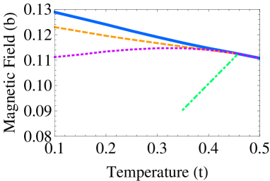
Figure 1: Phase transition lines for a 3D system with s-wave pairing : N-SC transitions for order parameters with (solid line) or without (doted line) FFLO modulation, and FFLO-BCS transitions obtained for GL free energy with (dashed line) or without (doted-dashed line) quartic correction. The N-SC transition is of second order whereas the FFLO-BCS transition is of first order. The value of the spin splitting parameter is $\sigma=1.8$.

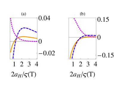
Figure 2: The GL coefficients (in arbitrary units ) $\beta\left(t,b,q=0\right)$ (dashed lines), $\frac{d\alpha\left(t,b,q=0\right)}{dq^{2}}$(solid lines) ,$\frac{d\beta\left(t,b,q=0\right)}{dq^{2}}$(doted lines) as functions of the parameter $\frac{2a_{H}}{\varsigma\left(T\right)}$ for (a) $v_{0}=.4$  and (b) $v_{0}=1$.

As we shall show below, the situation $T_{fflo}>T^{\ast}$, where $T^{\ast}$ is the temperature at which $\beta\left(t,b_{c2},q=0\right)=0$ , is realized in 3D systems (corresponding to $v_{0}=1$), regardless of the spin-splitting strength and the type of electron pairing.  A typical phase diagram is shown in Fig. 1 for $s$-wave pairing and spin pair-breaking parameter $\sigma=3$.

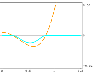
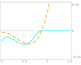
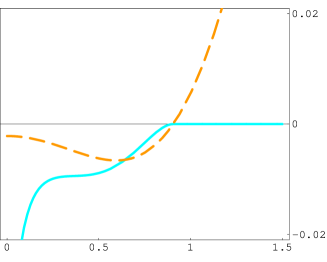
$\widetilde{q}$

Figure 3: (a) The dependence of the GL coefficient $\alpha$ (orange) and the mean field SC free energy, $-\theta\left(\alpha\right)\frac{\alpha^{2}}{2\beta_{A}\beta}$ (blue), on the modulation paramer,  $\widetilde{q}\equiv\left(\frac{2}{\sigma}\right)\sqrt{\frac{m^{\ast}}{m_{z}^{\ast}}}\left(qa_{H_{c20}^{orb}}\right)$, in a 3D system ($v_{0}=1$) , at $t=0.4$, $b=0.1142$, i.e. near the tricritical point, just below the Normal-nonuniform SC transition. It is seen that $\alpha<0$ in a small region around $\ \widetilde{q}=0.6$ where the SC free energy has a minimum. The value of the spin splitting parameter is $\sigma=3$. (b): The same as in (a) but for a slightly lower field, $b=0.114$, where a uniform ($q=0$) metastable SC state is present. (c): The same as in (b) but for a slightly lower field, $b=0.1139$, where a uniform ($q=0$) equilibrium SC state is present, while a metastable SC state exists at $q\not=0$.

As long as $T>T^{\ast}$ (so that $\beta\left(t,b_{c2},q=0\right)>0$) the normal to SC (N-SC) phase transition is of second-order and the (reduced) critical field, $b_{c2}\left(t\right)$, can be determined as the maximal value of $b\equiv H/H_{c20}^{orb}$ obtained from the equation $\alpha\left(t,b,q\right)=0$ for all values of $q$ , at the (reduced) temperature $t\equiv T/T_{c0}$. The solution of this equation for $q=0$ yields a transition line, $b=b_{c2}^{\left(0\right)}\left(t\right)$, ignoring the possibility of a FFLO state. The tricritical point, $T_{fflo}$, is defined as the maximal temperature at which $b_{c2}\left(t\right)>b_{c2}^{\left(0\right)}\left(t\right)$. It can alternatively be determined from the equation $\frac{d\alpha\left(t,b_{c2},q=0\right)}{dq^{2}}=0$ , which is equivalent to the condition for vanishing of the coefficient of $\left|\nabla\Delta\right|^{2}$ in a gradient expansion of the SC free energyhouzet01 .

For $T<T^{\ast}$ and sufficiently strong spin pair-breaking there can be a changeover to first-order SC transitions, but since $\beta\left(t,b_{c2},q\neq 0\right)>\beta\left(t,b_{c2},q=0\right)$ (see Fig.2 ), the segment of the $b_{c2}\left(t\right)$-line with first order transitions arises only at very low temperatures. For moderate $\sigma$ values the coefficient $\beta\left(t,b_{c2},q\right)$ at optimal $q$ is always positive and the N-SC transition is of the second order at arbitrarily low temperature.

The transition within the SC region from the nonuniform (FFLO) to uniform (BCS) phase at $T>T^{\ast}$ can not be obtained just by analyzing the quadratic term $\alpha\left(t,b,q\right)$ since the SC order parameter is finite there. It can be obtained by minimizing the SC free energy (including both quadratic and quartic terms) with respect to the modulation wave number $q$.  Neglecting the sixth and higher order terms in the expansion, the corresponding (standard) GL free energy, $\Omega\left(q\right)\simeq-\theta\left(\alpha\right)\frac{\alpha^{2}}{2\beta}$, ( $\theta\left(\alpha\right)$ being the Heaviside step function), which has a single minimum at $q\not=0$ for field near $b_{c2}$ (see Fig. 3a), developes a double-well structure (see Fig. 3b) as a function of $q$ upon decreasing the field below $b_{c2}$ at a given temperature $T$ (due to the symmetry $q\leftrightarrow-q$ only positive values may be considered). One of these minima is always at $q=0$, and it becomes energetically favorable at a critical field for a first order phase transition from the FFLO to the uniform BCS phase. The second (metastable) minimum at $q\not=0$ disappears completely upon further field decrease (see Fig. 3c).

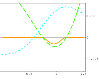
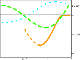
$\widetilde{q}$

Figure 4: The GL coefficients, $\alpha$ (green) and $\beta$ (blue), and the mean field SC free energy (orange) as functions of the modulation parameter, $\widetilde{q}$, in a 3D system ($v_{0}=1$) at a relatively low temperature $t=.25$ and decreasing field values (a) $b=.118$ and (b) $b=.117$. Note the vanishing of $\beta$ inside the region where $\alpha<0$ , around which the used approximation, $-\theta\left(\alpha\right)\frac{\alpha^{2}}{2\beta_{A}\beta}$, for $\Omega(q)$ breaks down (dashed sector of the orange line ).

At temperatures $T$ below $T^{\ast}$ the first two terms in the expansion of the thermodynamic potential are not sufficient to correctly describe the uniform SC state since for negative $\beta$- values the scale of the SC free energy is determined by the sixth order term. In contrast, the free energy of the nonuniform state, where $\beta\left(t,b,q\not=0\right)>0$, can be obtained from the stantard GL functional (with the assumption that the contribution of the sixth order term is small compared to that of the quartic term). The characteristic $q$-dependences of the GL coefficients, $\alpha$ and $\beta$, and the mean field free energy $-\theta\left(\alpha\right)\frac{\alpha^{2}}{2\beta_{A}\beta}$, for $T<T^{\ast}$ are illustrated in Fig. 4. Whereas at high fields (Fig. 4a) the minimum of the SC energy occurs in a region where $\beta>0$, at lower fields (see Fig. 4b) it approaches the expanding temperature domain of negative $\beta$. Thus, even for moderate spin splitting and low temperature the transition line from the nonuniform to uniform SC state cannot be determined without knowing the sixth-order term. It is clear, however, that this transition is of the first order.

It should be noted that if one attempts to determine the FFLO-BCS phase boundary from the equation $\frac{d\alpha\left(t,b,q=0\right)}{dq^{2}}=0$ it will greatly overestimate the size of the FFLO phase as compared to that obtained by minimizing $-\frac{\alpha^{2}}{2\beta}$ (see Fig. 1). This remarkable difference is due to the strong $q^{2}$-dependence of the quartic coefficient $\beta$ (see Fig.2).

The suppression of the orbital effect in the considered 3D systems, with ellipsoidal Fermi surfaces contained entirely within the BZ, is due to the factor $1-v^{2}$ appearing in the Gaussian exponents of Eqs. (40),(41). The recovery of this effect in quasi-2D systems with truncated ellipsoidal Fermi surface, where $v_{0}<1$, can reverse the relation between $T_{fflo}$ and $T^{\ast}$. Fig. 2b, where the GL coefficients are shown for $\sigma=1.8$, $v_{0}=.4$ and $s$-wave pairing, illustrates the situation with $T_{fflo}<T^{\ast}$, which occurs for all values of $v_{0}$ below a critical dimensionality $v_{0,cr}\approx 0.44$ (see Fig. 5), and depends only weakly on the spin-splitting parameter $\sigma$.

Figure 5: Solutions$\ \frac{2a_{H}}{\varsigma\left(T\right)}\propto T$ of the equation $\beta\left(q=0\right)=0$, corresponding to $T^{\ast}$ (dashed line), and the equation $\frac{d\alpha\left(q=0\right)}{dq^{2}}=0$, corresponding to $T_{fflo}$ (solid line) vs the dimensionality crossover parameter $v_{0}$ for $\sigma=2.5$.

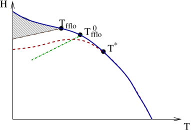
Figure 6: Schematic phase diagram for a quasi 2D system. The shaded area corresponds to a nonuniform SC (FFLO) phase, the dashed line corresponds to $\alpha\left(t,b,q=0\right)=0$ , and the dotted-dashed line can be obtained from $\frac{d}{dq^{2}}\alpha\left(t,b,q=0\right)=0$.

The corresponding phase diagram (see Fig. 6 ) for $v_{0}$ below this crossing point is quite different from that found for the 3D systems shown in Fig.1. First of all, since $\beta<0$ , one may use Eqs. (40),(41) to determine the phase diagram only under the assumption that the sixth order coefficient $\gamma$ is positive (see Ref.adachi03 ). In this case a discontinuous SC transition occurs at $\Omega\left(\Delta_{0}^{2}\right)=0$ with $\Delta_{0}^{2}=\left(\frac{3\left|\beta\right|}{4\gamma}\right)$ and $\alpha=\frac{3\beta^{2}}{16\gamma}>0$ , and the corresponding critical field, $b_{c2}(t)$ , should be larger than $b_{c2}^{0}\left(t\right)$ , obtained from the equation $\alpha(q=0)=0$.  Thus, at a temperature below $T^{\ast}$, the N-SC phase boundary includes a segment of first order transitions, which may end at zero temperature, or at a finite temperature, depending on the spin-splitting strength. This dependence appears because of the competition between the decreasing explicit dependence of $\beta$ on decreasing temperature and its increasing implicit dependence through $q\left(T\right)$ at the FFLO state.  The boundary between the BCS and FFLO states should be determined by minimizing the free energy, Eq. (39), with respect to $q$. This may be restricted to the explicit dependence on $q$ since the order parameter is determined by: $\frac{\partial\Omega}{\partial\Delta^{2}}=0$. Consequently the positive sign of $\frac{d\beta\left(t,b,q=0\right)}{dq^{2}}$ (see Fig. 2b) results in partial cancellation of the leading contribution to $\frac{\partial\Omega}{\partial q^{2}}$, which is proportional to $\frac{d\alpha\left(t,b,q=0\right)}{dq^{2}}$ and negative in the FFLO part of the phase diagram. Moreover, since for the discontinuous transition the order parameter is finite just below the transition the higher order terms in $\Delta_{0}^{2}$ (Eq. (39)) should be taken into account. As a result $T_{fflo}$ should be smaller than $T_{fflo}^{0}$- the temperature obtained from the equation $\frac{d\alpha\left(t,b,q=0\right)}{dq^{2}}$ $=0$ , as schematically shown in Fig. 6.

IV Conclusions

It is shown that the expected changeover to first-order SC transitions in clean, strongly type-II superconductors in the Pauli paramagnetic limit can take place only in materials with quasi-cylindrical Fermi surfaces, regardless of the type of the electron (s or d-wave) pairing interaction which leads to superconductivity. This finding clarifies the confusing current literature on this topicgruenberg66 ,houzet01 ,adachi03 .

The observation of such a changeover in the heavy fermion compound CeCoIn₅ for magnetic field orientation perpendicular to the easy conducting planeBianchi0203 is consistent with the quasi-2D character of its electronic band structure Settai01 . The interesting situation of a 2D superconductor under a magnetic field parallel to the conducting plane, for which a changeover to discontinuous SC transitions was reported very recentlyLortz07 , is more subtle since the vanishingly small cyclotron frequency characterizing this case does not allow utilization of the Landau orbitals approach employed here (for a recent review see, e.g.Matsuda-Shimahara07 ).

Acknowledgements: This research was supported by the Israel Science Foundation founded by the Academy of Sciences and Humanities, by the Argentinian Research Fund at the Technion, and by EuroMagNET under the EU contract RII3-CT-2004-506239.

References

- (1) 1. K.H. Bennemann and J.B. Ketterson (Eds.) The Physics of Superconductors, Vol. I and Vol. II (Springer, Berlin 2003 and 2004).
- (2) C. Petrovic et al. Europhys. Lett. 53, 354 (2001).
- (3) I. Ishiguro and K. Yamaji, Organic Superconductors ( Springer-Verlag, Berlin Heidelberg 1990).
- (4) J. Wosnitza, Fermi Surfaces of Low-Dimensional Organic Metals and Superconductors (Springer, Berlin 1996).
- (5) K. Izawa et al., Phys. Rev. Lett., 87, 057002 (2001).
- (6) A.M. Clogston, Phys. Rev. Lett. 9, 593 (1962).
- (7) B.S. Chandrasekhar, Appl. Phys. Lett. 1, 7 (1962).
- (8) G. Sarma, J. Phys. Chem. Solids 24 , 1029 (1963).
- (9) K. Maki and T. Tsuneto, Prog. Theor. Phys. 31, 945 (1964).
- (10) P. Fulde in Superconductivity (Proceeding of the Advanced Summer Study Institute on Superconductivity, McGill University, 1968), ed. P.R. Wallace (Gordon and Breach , NY), p. 535.
- (11) A. Bianchi, R. Movshovich, N. Oeschler, P. Gegenwart, F. Steglich, J.D. Tompson, P.G. Pagliuso, and J.L. Sarrao, Phys. Rev. Lett. 89, 137002 (2002); Phys. Rev. Lett. 91, 187004 (2003).
- (12) R. Lortz, Y Wang, A. Demuer, M. Bottger, B. Bergk, G. Zwicknagl, Y. Nakazawa, and J. Wosnitza , cond-mat/0706.3584
- (13) P. Fulde and R.A. Ferrell, Phys. Rev. 135, A550, (1964).
- (14) A.I. Larkin and Yu.N. Ovchinnikov, Zh. Eksp. Teor. Fiz. 47, 1136 (1964) [Sov. Phys. JETP 20, 762 (1965)]
- (15) D. Saint-James, G. Sarma, and E.J. Thomas, Type II superconductivity (Pergamon, New York, 1969.
- (16) D.F. Agterberg and K. Yang, J. Phys.: Condens. Matter 13, 9259 (2001).
- (17) L.W. Gruenberg and L. Gunter, Phys. Rev. Lett. 16, 966 (1966).
- (18) M. Houzet and A. Buzdin, Phys. Rev. B 63, 184521 (2001).
- (19) H. Adachi and R. Ikeda, Phys. Rev. B 68, 184510 (2003).
- (20) R. Settai, H. Shishido, S. Ikeda, M. Nakashima, D. Aoki, Y. Haga, H. Harima, Y. Onuki, Physica B 312-313, 123 (2002).
- (21) H. Shishido et al., J. Phys.: Condens. Matter 15, L499 (2003).
- (22) M. Rasolt and Z. Tesanovic, Rev. Mod. Phys., 64, 709 (1992).
- (23) T. Maniv, R. Rom, I.D. Vagner, and P. Wyder, Phys. Rev. B 46 , 8360 (1992).
- (24) Y. A. Bychkov and L. P. Gorkov, Sov. Phys. JETP 14 , 1132 (1962).
- (25) T. Maniv, V. Zhuravlev, I. D. Vagner, and P. Wyder, Rev. Mod. Phys.,73, 867.
- (26) M. J. Stephen, Phys. Rev. B 45 , 5481 (1992).
- (27) V. Zhuravlev and V. Shapiro, HAIT Jour. Sci. Tech. 1 (4) 707-720 (2004).
- (28) N.R. Werthamer, in Superconductivity ed R.D. Parks (Dekker, New-York 1969).
- (29) M. G. Vavilov, and V. P. Mineev, JETP 85, 1024 (1997).
- (30) E. Helfand and N.R. Werthamer, Phys. Rev. 147, 288 (1966), N.R. Werthamer, E. Helfand, and P.C. Hohenberg, 147, 295 (1966).
- (31) V. Zhuravlev, T. Maniv, I. D. vagner, and P. Wyder, Phys. Rev. B 56 , 14693 (1997).
- (32) R. Settai, H. Shishido, S. Ikeda, Y. Murakawa, M. Nakashima, D. Aoki, Y. Haga, H. Harima and Y. Onuki, J. Phys.: Cond. Matt. 13 , L627-634 (2001).
- (33) Y. Matsuda and H. Shimahara, J. Phys. Soc. Jpn. 76, 051005 (2007).