Distributed Slicing in Dynamic Systems

Abstract

Peer to peer (P2P) systems are moving from application specific architectures to a generic service oriented design philosophy. This raises interesting problems in connection with providing useful P2P middleware services capable of dealing with resource assignment and management in a large-scale, heterogeneous and unreliable environment. The slicing service, has been proposed to allow for an automatic partitioning of P2P networks into groups (slices) that represent a controllable amount of some resource and that are also relatively homogeneous with respect to that resource. In this paper we propose two gossip-based algorithms to solve the distributed slicing problem. The first algorithm speeds up an existing algorithm sorting a set of uniform random numbers. The second algorithm statistically approximates the rank of nodes in the ordering. The scalability, efficiency and resilience to dynamics of both algorithms rely on their gossip-based models. These algorithms are proved viable theoretically and experimentally.

Keywords: Slice, Gossip, Churn, Peer-to-Peer, Aggregation, Large Scale.

1 . Introduction

1.1 . Context and Motivations

The peer to peer (P2P) communication paradigm has now become the prevalent model to build large-scale distributed applications. On the one hand, P2P protocols integrate into platforms on top of which several applications, with various requirements, may cohabit. This leads to the interesting issue of resource assignment or how to allocate a set of nodes for a given application. Examples of applications for such a service are telecommunication, testbed platform [3], or desktop-grid-like applications [2]. On the other hand, P2P systems should be able to balance the load taking into account that capabilities are heterogeneous at the peers [19, 4, 20]. This heterogeneity has some drawbacks. Completely decentralized P2P application, like the original Gnutella [8], suffered from congestion when applied to large-scale systems because nodes with a low bandwidth capability were queried. Consequently, file sharing applications [16, 9] tend to request ultrapeers/supernodes (peers with larger lifetime and bandwidth capabilities), more often than regular peers. P2P protocols must identify efficiently and accurately peers with specific capabilities.

Large scale dynamic distributed systems consist of many participants that can join and leave at will. Identifying peers in such systems that have a similar level of power or capability (for instance, in terms of bandwidth, processing power, storage space, or uptime) in a completely decentralized manner is a difficult task. It is even harder to maintain this information in the presence of churn. Due to the intrinsic dynamics of contemporary P2P systems it is impossible to obtain accurate information about the capabilities (or even the identity) of the system participants. Consequently, no node is able to maintain accurate information about all the nodes. This disqualifies centralized approaches.

The slicing service [13] enables peers to self-organize into a partitioning, where partitions (slices) are connected overlay networks that represent a given percentage of some resource. The slicing is ordered in the sense that peers are sorted according to their capabilities expressed by an attribute value. Building upon the work on ordered slicing of [13], here we focus on the issue of accurate slicing. That is, we focus on improving quality by slicing the network accurately, and improving stability of slices by minimizing the impact of the churn. The distributed slicing problem we tackle in this paper consists in ranking nodes depending on their relative capability, slicing the network depending on these capabilities and, most importantly, readapting the slices continuously to cope with system dynamism.

1.2 . Contributions

The paper presents two distributed algorithms to slice the nodes according to their capability, reflected by an attribute value. Theses algorithms are robust and lightweight due to their gossip-based communication pattern. The first algorithm of the paper builds upon the ordered slicing algorithm proposed in [13] that we call the JK algorithm in the sequel of this paper. This algorithm speeds up the convergence of JK by locally computing a disorder measure so that a peer chooses the neighbor to communicate with in order to maximize the chance of decreasing the global disorder measure.

Then, we identify two issues that prevent accurate slicing and motivate us to find an alternative approach to this algorithm and JK. First, the slicing might be inaccurate. Random values are used to calculate which slice a node belongs to. The accuracy of the slicing fully depends on the uniformity of the random value spread between 0 and 1. (e.g., the proportion of random values between 0.8 and 1 should be ideally 20% of the nodes). Second, the previous algorithms suffer from churn an dynamism when correlated with the attribute values. For example, if the peers are sorted according to their connectivity potential, a portion of the attribute space (and therefore the random value space) might be suddenly affected. The consequence is to skew the distribution of random values towards high or low values.

The second algorithm is an alternative algorithm solving these two issues by approximating locally the rank of the nodes, without using random values. The basic idea is that each node periodically estimates its rank along the attribute axis depending on the attributes it have seen so far. Based on continuously aggregated information, the node can determine the slice it belongs to with a decreasing error margin. We show that this algorithm provides accurate estimation and recovery ability in presence of attributes-correlated churn at the price of a slower convergence.

1.3 . Outline

The rest of the paper is organized as follows: Section 2 surveys some related work. The system model is presented in Section 3. The first contribution of an improved ordered slicing algorithm based on random values is presented in Section 4 and the second algorithm based on dynamic ranking in Section 5. Section 6 concludes the paper.

2 . Related Work

Most of the solutions proposed so far for ordering nodes come from the context of databases [5, 11], where parallelizing query executions is used to improve efficiency. A large majority of the solutions in this area rely on centralized gathering or all-to-all exchange, which makes them unsuitable for large-scale networks.

Other related problems are the selection problem and the $\phi$-quantile search. The selection problem [7] aims at determining the $i^{th}$ smallest element with as few comparisons as possible. The $\phi$-quantile search (with $\phi\in(0,1]$) is the problem to find among $n$ elements the $(\phi n)^{th}$ element. Even though these problems look similar to our problem, they aim at finding a specific node among all, while the distributed slicing problem aims at solving a global problem where each node maintains a piece of information. Additionally, solutions to the quantile search problem like the one presented in [17] use an approximation of the system size. The same holds for the algorithm in [18], which uses similar ideas to determine the distribution of a utility in order to isolate peers with high capability—i.e., super-peers.

As far as we know, the distributed slicing problem was studied in a P2P system for the first time in [13]. In this paper, every node draws independently and uniformly a random value in the interval $(0,1]$. Each of these values serve as an estimate of normalized index $k/n$ for the node with the $k^{th}$ smallest attribute value.

3 . Model and Problem Statement

3.1 . System model

We consider a system $\Sigma$ containing a set of $n$ uniquely identified nodes.(The value $n$ may vary over time.) The set of identifiers is denoted by $I\subset\mathbb{N}$. Each node can leave and new nodes can join the system at any time, thus the number of nodes is a function of time. Nodes may also crash. In this paper, we do not differentiate between a crash and a voluntary node departure.

Each node $i$ maintains a fixed attribute value $a_{i}\in\mathbb{N}$, reflecting the node capability according to a specific metric. These attribute values over the network might have an arbitrary skewed distribution. Initially, a node has no global information neither about the structure or size of the system nor about the attribute values of the other nodes.

We can define a total ordering over the nodes based on their attribute value, with the node identifier used to break ties. Formally, we let $i$ precede $j$ if and only if $a_{i}<a_{j}$, or $a_{i}=a_{j}$ and $i<j$. We refer to this totally ordered sequence as the attribute-based sequence, denoted by $A.\mathord{\it sequence}$. The attribute-based rank of a node $i$, denoted by $\alpha_{i}\in\{1,...,n\}$, is defined as the index of $a_{i}$ in $A.\mathord{\it sequence}$.

3.2 . Distributed Slicing Problem

Let ${\cal S}_{l,u}$ denote the slice containing every node $i$ whose normalized rank, namely $\frac{\alpha_{i}}{n}$, satisfies $l<\frac{\alpha_{i}}{n}\leq u$ where $l\in[0,1)$ is the slice lower boundary and $u\in(0,1]$ is the slice upper boundary so that all slices represent adjacent intervals $(l_{1},u_{1}],(l_{2},u_{2}]$… Let us assume that we partition the interval $(0,1]$ using a set of slices, and this partitioning is known by all nodes. The distributed slicing problem requires each node to determine the slice it currently belongs to. Note that the problem stated this way is similar to the ordering problem, where each node has to determine its own index in $A.\mathord{\it sequence}$. However, the reference to slices introduces special requirements related to stability and fault tolerance, besides, it allows for future generalizations when one considers different types of categorizations.

Figure 1 illustrates an example of a population of 10 persons, to be sorted against their height. A partition of this population could be defined by two slices of the same size: the group of short persons, and the group of tall persons. This is clearly an example where the distribution of attribute values is skewed towards 2 meters. The rank of each person in the population and the two slices are represented on the bottom axis. Each person is represented as a small cross on these axes. Each slice is represented as an oval. The slice $S_{1}={\cal S}_{0,\frac{1}{2}}$ contains the five shortest persons and the slice $S_{2}={\cal S}_{\frac{1}{2},1}$ contains the five tallest persons.

Figure 1: Slicing of a population based on a height attribute.

Since the distribution of attribute values is unknown and hard to predict, defining relevant groups is a difficult task. For example, if the distribution of the human heights were unknown, then the persons taller than $1m$ could be considered as tall and the persons shorter than $1m$ could be considered as short. In this case, the first of the two groups would be empty, while the second of the two groups would be as big as the whole system. Conversely, slices partition the population into subsets representing a predefined portion of this population. Therefore, in the rest of the paper, we consider slices as defined as a proportion of the network.

3.3 . Facing Churn

Node churn, that is, the continuous arrival and departure of nodes is an intrinsic characteristic of P2P systems and may significantly impact the outcome, and more specifically the accuracy of the slicing algorithm. The easier case is when the distribution of the attribute values of the departing and arriving nodes are identical. In this case, in principle, the arriving nodes must find their slices, but the nodes that stay in the system are mostly able to keep their slice assignment. Even in this case however, nodes that are close to the border of a slice may expect frequent changes in their slice due to the variance of the attribute values, which is non-zero for any non-constant distribution. If the arriving and departing nodes have different attribute distributions, so that the distribution in the actual network of live nodes keeps changing, then this effect is amplified. However, we believe that this is a realistic assumption to consider that the churn may be correlated with some specific values (for example if the considered attribute is uptime or connectivity).

4 . Dynamic Ordering by Exchange of Random Values

This section proposes an algorithm for the distributed slicing problem improving upon the original JK algorithm [13], by considering a local measure of the global disorder function. In this section we present the algorithm along with the corresponding analysis and simulation results.

4.1 . On Using Random Numbers to Sort Nodes

This Section presents the algorithm built upon JK. We refer to this algorithm as mod-JK (standing for modified JK). In JK, each node $i$ generates a real number $r_{i}\in(0,1]$ independently and uniformly at random. The key idea is to sort these random numbers with respect to the attribute values by swapping (i.e., exchanging) these random numbers between nodes, so that if $a_{i}<a_{j}$ then $r_{i}<r_{j}$. Eventually, the attribute values (that are fixed) and the random values (that are exchanged) should be sorted in the same order. That is, each node would like to obtain the $x^{th}$ largest random number if it owns the $x^{th}$ largest attribute value. Let $R.\mathord{\it sequence}$ denote the random sequence obtained by ordering all nodes according to their random number. Let $\rho_{i}(t)$ denote the index of node $i$ in $R.\mathord{\it sequence}$ at time $t$. When not required, the time parameter is omitted.

Once sorted, the random values are used to determine the portion of the network a peer belongs to.

4.2 . Definitions

Every node $i$ keeps track of some neighbors and their age. The age of neighbor $j$ is a timestamp, $t_{j}$, set to 0 when $j$ becomes a neighbor of $i$. Thus, node $i$ maintains an array containing the id, the age, the attribute value, and the random value of its neighbors. This array, denoted ${\mathcal{N}}_{i}$, is called the view of node $i$. The views of all nodes have the same size, denoted by $c$. A node $i$ participates in the algorithm by exchanging its rank with a misplaced neighbor in its view. Neighbor $j$ is misplaced if and only if $(a_{j}-a_{i})(r_{j}-r_{i})<0$. In [13], a measure of the relative disorder of sequence $R.\mathord{\it sequence}$ with respect to sequence $A.\mathord{\it sequence}$ was introduced. We call it the global disorder measure (GDM) and it is defined, for any time $t$, as $\mathord{\it GDM}(t)=\frac{1}{n}\sum_{i}(\alpha_{i}-\rho(t)_{i})^{2}.$ The minimal value of GDM is 0, which is obtained when $\rho(t)_{i}=\alpha_{i}$ for all nodes $i$. In this case the attribute-based index of a node is equal to its random value index, indicating that random values are ordered.

4.3 . Improved Ordering Algorithm

In this algorithm, each node $i$ searches its own view ${\mathcal{N}}_{i}$ for misplaced neighbors. Then, one of them is chosen to swap random value with. This process is repeated until there is no global disorder. In this version of the algorithm, we provide each node with the capability of measuring disorder locally. This leads to a new heuristic for each node to determine the neighbor to exchange with which decreases most the disorder. Referring to this disorder measure as a criterion, the decrease of the global criterion is related to the decrease of local criteria, similarly to [1].

For a node $i$ to evaluate the gain of exchanging with a node $j$ of its current view ${\mathcal{N}}_{i}$, we define its local disorder measure (abbreviated LDM_i). Let $LA.\mathord{\it sequence}_{i}$ and $LR.\mathord{\it sequence}_{i}$ be the local attribute sequence and the local random sequence of node $i$, respectively. These sequences are computed locally by $i$ using the information ${\mathcal{N}}_{i}\cup\{i\}$. Similarly to $A.\mathord{\it sequence}$ and $R.\mathord{\it sequence}$, these are the sequences of neighbors where each node is ordered according to its attribute value and random number, respectively. Let, for any $j\in{\cal N}_{i}\cup\{i\}$, $\ell\rho_{j}(t)$ and $\ell\alpha_{j}(t)$ be the indices of $r_{j}$ and $a_{j}$ in sequences $LR.\mathord{\it sequence}_{i}$ and $LA.\mathord{\it sequence}_{i}$, respectively, at time $(t)$. At any time $t$, the local disorder measure of node $i$ is defined as:

$$\mathord{\it LDM}_{i}(t) = \frac{1}{c+1}\sum_{j\in{\mathcal{N}}_{i}(t)\cup\{i\}}(\ell\alpha_{j}(t)-\ell\rho_{j}(t))^{2}.$$ (1)

We denote by $G_{i,j}(t+1)=\mathord{\it LDM}_{i}(t)-\mathord{\it LDM}_{i}(t+1)$, the reduction on this measure that $i$ obtains after exchanging its random value with node $j$ between time $t$ and $t+1$.

The heuristic used chooses for node $i$ the misplaced neighbor $j$ that maximizes $G_{i,j}(t+1)$.

Sampling uniformly at random.

The algorithm relies on the fact that potential misplaced nodes are found so that they can swap their random numbers thereby increasing order. If the global disorder is high, it is very likely that any given node has misplaced neighbors in its view to exchange with. Nevertheless, as the system gets ordered, it becomes more unlikely for a node $i$ to have misplaced neighbors. In this stage the way the view is composed plays a crucial role: if fresh samples from the network are not available, convergence can be slower than optimal.

Several protocols may be used to provide a random and dynamic sampling in a P2P system such as Newscast [15], Cyclon [21] or Lpbcast [12]. They differ mainly by their closeness to the uniform random sampling of the neighbors and the way they handle churn. In this paper, we chose to use a variant of the Cyclon protocol, to construct and update the views, as it is reportedly the best approach to achieve a uniform random neighbor set for all nodes [10].

Description of the algorithm.

The algorithm is presented in Figure 2. The active thread at node $i$ runs the membership (gossiping) procedure ($\mathord{\sf recompute-view}()_{i}$) and the exchange of random values periodically. As motivated above, the membership procedure is similar to the Cyclon algorithm. This variant of Cyclon exchanges all entries of the view at each step and uses two additional parameters: the attribute value and the random value. For the detailed pseudocode, please refer to the full version of this paper [6].

Initial state of node $i$ (1) $\mathord{\it period}_{i}$, initially set to a constant; $r_{i}$, a random value chosen in $(0,1]$; $a_{i}$, the attribute value; $\mathord{\it slice}_{i}\leftarrow\bot$, the slice $i$ belongs to; ${\mathcal{N}_{i}}$, the view; $\mathord{\it gain}_{j^{\prime}}$, a real value indicating the gain achieved by exchanging with $j^{\prime}$; $\mathord{\it gain-max}=0$, a real. Active thread at node $i$ (2) $\mathord{\sf wait}(\mathord{\it period_{i}})$ (3) $\mathord{\sf recompute-view}()_{i}$ (4) for $j^{\prime}\in{\mathcal{N}}_{i}$ (5) if $\mathord{\it gain}_{j^{\prime}}\geq\mathord{\it gain-max}$ then (6)         $\mathord{\it gain-max}\leftarrow\mathord{\it gain}_{j^{\prime}}$ (7)         $j\leftarrow j^{\prime}$ (8) end for (9) $\mathord{\sf send}(\mathord{\sf REQ},r_{i},a_{i})$ to $j$ (10) $\mathord{\sf recv}(\mathord{\sf ACK},r_{j}^{\prime})$ from $j$ (11) $r_{j}\leftarrow r_{j}^{\prime}$ (12) if $(a_{j}-a_{i})(r_{j}-r_{i})<0$ then (13) $r_{i}\leftarrow r_{j}$ (14) $\mathord{\it slice}_{i}\leftarrow{\cal S}_{l,u}$ such that $l<r_{i}\leq u$ Passive thread at node $i$ activated upon reception (15) $\mathord{\sf recv}(\mathord{\sf REQ},r_{j},a_{j})$ from $j$ (16) $\mathord{\sf send}(\mathord{\sf ACK},r_{i})$ to $j$ (17) if $(a_{j}-a_{i})(r_{j}-r_{i})<0$ then (18) $r_{i}\leftarrow r_{j}$ (19) $\mathord{\it slice}_{i}\leftarrow{\cal S}_{l,u}$ such that $l<r_{i}\leq u$

Figure 2: Dynamic ordering algorithm.

The algorithm for exchanging random values from node $i$ starts by measuring the ordering that can be gained by swapping with each neighbor (Lines 2–2). Then, $i$ chooses the neighbor $j\in{\mathcal{N}}_{i}$ that maximizes gain $G_{i,k}$ for any of its neighbor $k$. Formally, $i$ finds $j\in{\mathcal{N}}_{i}$ such that for any $k\in{\mathcal{N}}_{i}$, we have

$$G_{i,j}(t+1)\geq G_{i,k}(t+1).$$

In Figure 2 of node $i$, we refer to $\mathord{\it gain}_{j}$ as the value of $\ell\alpha_{i}(t)\ell\rho_{j}(t)+\ell\alpha_{j}(t)\ell\rho_{i}(t)-\ell\alpha_{j}(t)\ell\rho_{j}(t)$. This expression is directly obtained from equation (1), see the full version of this paper [6] for furthter details.

From this point on, $i$ exchanges its random value $r_{i}$ with the random value $r_{j}$ of node $j$ (Line 2). The passive threads are executed upon reception of a message. In Figure 2, when $j$ receives the random value $r_{i}$ of node $i$, it sends back its own random value $r_{j}$ for the exchange to occur (Lines 2–2). Observe that the attribute value of $i$ is also sent to $j$, so that $j$ can check if it is correct to exchange before updating its own random number (Lines 2–2). Node $i$ does not need to receive attribute value $a_{j}$ of $j$, since $i$ already has this information in its view and the attribute value of a node never changes over time.

4.4 . Analysis of Slice Inaccuracy

In mod-JK, as in JK, the current random number $r_{i}$ of a node $i$ determines the slice $s_{i}$ of the node. The objective of both algorithms is to reduce the global disorder as quickly as possible. Algorithm mod-JK consists in choosing one neighbor among the possible neighbors that would have been chosen in JK, plus the GDM of JK has been shown to fit an exponential decrease. Consequently mod-JK experiences also an exponential decrease of the global disorder. Eventually, JK and mod-JK ensure that the disorder has fully disappeared. For further information, please refer to [13].

However, the accuracy of the slices heavily depends on the uniformity of the random value spread between 0 and 1. It may happen, that the distribution of the random values is such that some peers decide upon a wrong slice. Even more problematic is the fact that this situation is unrecoverable unless a new random value is drawn for all nodes. This may be considered as an inherent limitation of the approach. For example, consider a system of size 2, where nodes 1 and 2 have the random values $r_{1}=0.1$, $r_{2}=0.4$. If we are interested in creating two slices $S_{1}$ and $S_{2}$ of equal size ($S_{1}={\cal S}_{0,\frac{1}{2}}$ and $S_{2}={\cal S}_{\frac{1}{2},1}$), both nodes will wrongly believe to belong to the same slice $S_{1}$, since $r_{1}$ and $r_{2}$ belong to $(0,\frac{1}{2}]$. This wrong estimate holds even after perfect ordering of the random values.

Therefore, an important step is to characterize the inaccuracy of slice assignment and how likely it may happen. To this end, we bound the deviation of random values distribution from the mean, and we lower bound the probability that this happen with only two slices. The following result bounds, with high probability, the number of nodes that can be misplaced in the system. For the proof of Lemma 4.1 please refer to the full version of this paper [6].

Lemma 4.1

For any $\beta\in(0,1]$, a slice $S_{p}$ of length $p\in(0,1]$ has a number of peers $X\in[(1-\beta)np,(1+\beta)np]$ with probability at least $1-\epsilon$ as long as $p\geq\frac{3}{\beta^{2}n}\ln(2/\epsilon)$.

To measure the effect discussed above during the simulation experiments, we introduce the slice disorder measure (SDM) as the sum over all nodes $i$ of the distance between the slice $i$ actually belongs to and the slice $i$ believes it belongs to. For example (in the case where all slices have the same size), if node $i$ belongs to the $1^{st}$ slice (according to its attribute value) while it thinks it belongs to the $3^{rd}$ slice (according to its rank estimate) then the distance for node $i$ is $|1-3|=2$. Formally, for any node $i$, let $S_{u_{i},l_{i}}$ be the actual correct slice of node $i$ and let $S_{\hat{u_{i}},\hat{l_{i}}}(t)$ be the slice $i$ estimates as its slice at time $t$. The slice disorder measure is defined as:

$$\mathord{\it SDM}(t)=\sum_{i}\frac{1}{u_{i}-l_{i}}\left|\frac{u_{i}+l_{i}}{2}-\frac{\hat{u_{i}}+\hat{l_{i}}}{2}\right|.$$

$\mathord{\it SDM}(t)$ is minimal (equals 0) if for all nodes $i$, we have $S_{\hat{u_{i}},\hat{l_{i}}}(t)=S_{u_{i},l_{i}}$.

4.5 . Simulation Results

We present simulation results using PeerSim [14], using a simplified cycle-based simulation model, where all messages exchanges are atomic, so messages never overlap. First, we compare the performance of the two algorithms: JK and mod-JK. Second, we study the impact of concurrency that is ignored by the cycle-based simulations.

Performance comparison.

We compare the time taken by these algorithms to sort the random values according to the attribute values (i.e., the node with the $j^{th}$ largest attribute value of the system value obtains the $j^{th}$ random value). In order to evaluate the convergence speed of each algorithm, we use the slice disorder measure as defined in Section 4.4.

We simulated $10^{4}$ participants in 100 equally sized slices (when unspecified), each with a view size $c=20$. Figure 3 presents the evolution of the slice disorder measure over time for JK, and mod-JK.

Figure 3: Slice disorder measure over time.

Figure 3 shows the slice disorder measure to compare the convergence speed of our algorithm to that of JK with 10 equally sized slices. Our algorithm converges significantly faster than JK. Note that none of the algorithm reaches zero SDM, since they are both based on the same idea of sorting randomly generated values. Besides, since they both used an identical set of randomly generated values, both converge to the same SDM. Note that for the sake of fairness, JK and mod-JK are compared using the same underlying view management protocol in our simulation: the variant of Cyclon.

Concurrency.

The simulations are cycle-based and at each cycle an algorithm step is done atomically so that no other execution is concurrent. More precisely, the algorithms are simulated such that in each cycle, each node updates its view before sending its random value or its attribute value. Given this implementation, the cycle-based simulator does not allow us to realistically simulate concurrency, and a drawback is that view is up-to-date when a message is sent. In the following we artificially introduce concurrency (so that view might be out-of-date) into the simulator and show that it has only a slight impact on the convergence speed.

Adding concurrency raises some realistic problems due to the use of non-atomic push-pull [12] in each message exchange. That is, concurrency might lead to other problems because of the potential staleness of views: unsuccessful swaps due to useless messages. Technically, the view of node $i$ might indicate that $j$ has a random value $r$ while this value is no longer up-to-date. This happens if $i$ has lastly updated its view before $j$ swapped its random value with another $j^{\prime}$. Moreover, due to asynchrony, it could happen that by the time a message is received this message has become useless. Assume that node $i$ sends its random value $r_{i}$ to $j$ in order to obtain $r_{j}$ at time $t$ and $j$ receives it by time $t+\delta$. With no loss of generality assume $r_{i}>r_{j}$. Then if $j$ swaps its random value with $j^{\prime}$ such that $r_{j}^{\prime}>r_{i}$ between time $t$ and $t+\delta$, then the message of $i$ becomes useless and the expected swap does not occur (we call this an unsuccessful swap).

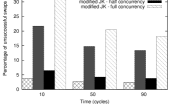
Figure 4: (a) Percentage of unsuccessful swaps. (b) Convergence speed under high concurrency.

Figure 4 indicates the impact of concurrent message exchange on the convergence speed. while Figure 4 shows the amount of useless messages that are sent. Now, we explain how the concurrency is simulated. Let the overlapping messages be a set of messages that mutually overlap: it exists, for any couple of overlapping messages, at least one instant at which they are both in-transit. For each algorithm we simulated (i) full concurrency: in a given cycle, all messages are overlapping messages; and (ii) half concurrency: in a given cycle, each message is an overlapping message with probability $\frac{1}{2}$. Generally, we see that increasing the concurrency increases the number of useless messages. Moreover, in the modified version of JK, more messages are ignored than in the original JK algorithm. This is due to the fact that some nodes (the most misplaced ones) are more likely targeted which increases the number of concurrent messages arriving at the same nodes. Since a node $i$ ignored more likely a message when it receives more messages during the same cycle, it comes out that concentrating message sending at some targets increases the number of useless messages.

Figure 4 compares the convergence speed under full concurrency and no concurrency. Full-concurrency impacts on the convergence speed very slightly.

5 . Dynamic Ranking by Sampling of Attributes

In this section we propose an alternative algorithm for the distributed slicing problem. This algorithm circumvents the problems identified in the previous approach by continuously ranking nodes based on observing attribute value information. Besides, this algorithm is not sensitive to churn even if it is correlated with attribute values. In the remaining part of the paper we refer to this new algorithm as the ranking algorithm while referring to JK and mod-JK as the ordering algorithms.

Impact of dynamics correlated with attribute.

As already mentioned, the ordering algorithms rely on the fact that random values are uniformly distributed. However, if the attribute values are not constant but correlated with the dynamic behavior of the system, the distribution of random values may change from uniform to skewed quickly. For instance, assume that each node maintains an attribute value that represents its own lifetime. Although the algorithm is able to quickly sort random values, so nodes with small lifetime will obtain the small random values, it is more likely that these nodes leave the system sooner than other nodes. This results in a higher concentration of high random values and a large population of the nodes wrongly estimate themselves as being part of the higher slices.

Inaccurate slice assignments.

As discussed in previous sections in detail, slice assignments will typically be imperfect even when the random values are perfectly ordered. Since the ranking approach does not rely on ordering random nodes, this problem is not raised: the algorithm guarantees eventually perfect assignment in a static environment.

Concurrency side-effect.

In the previous ordering algorithms, a non negligible amount of messages are sent unnecessarily. The concurrency of messages has a drastic effect on the number of useless messages as shown previously, slowing down convergence. In the ranking algorithm concurrency has no impact on convergence speed because all received messages are taken in account. This is because the information encapsulated in a message (the attribute value of a node) is guaranteed to be up to date, as long as the attribute values are constant.

5.1 . Ranking Algorithm Specification

The pseudocode of the ranking algorithm is presented in Figure 5. As opposed to the ordering algorithm of the previous section, the ranking algorithm does not assign random initial unalterable values as candidate ranks. Instead, the ranking algorithm improves its rank estimate each time a new message is received.

The ranking algorithm works as follows. Periodically each node $i$ updates its view ${\mathcal{N}}_{i}$ following an underlying protocol that provides a uniform random sample (Line 5); later, we simulate the algorithm using a variant of Cyclon protocol. See [6] for further details. Node $i$ computes its rank estimate (and hence its slice) by comparing the attribute value of its neighbors to its own attribute value. This estimate is set to the ratio of the number of nodes with a lower attribute value that $i$ has seen over the total number of nodes $i$ has seen (Line 5). Node $i$ looks at the normalized rank estimate of all its neighbors. Then, $i$ selects the node $j_{1}$ closest to a slice boundary (according to the rank estimates of its neighbors). Node $i$ selects also a random neighbor $j_{2}$ among its view (Line 5). When those two nodes are selected, $i$ sends an update message, denoted by a flag $\mathord{\sf UPD}$, to $j_{1}$ and $j_{2}$ containing its attribute value (Line 5–5).

The reason why a node close to the slice boundary is selected as one of the contacts is that such nodes need more samples to accurately determine which slice they belong to (subsection 5.2 shows this point). This technique introduces a bias towards them, so they receive more messages.

Upon reception of a message from node $i$, the passive threads of $j_{1}$ and $j_{2}$ are activated so that $j_{1}$ and $j_{2}$ compute their new rank estimate $r_{j_{1}}$ and $r_{j_{2}}$. The estimate of the slice a node belongs to, follows the computation of the rank estimate. Messages are not replied, communication is one-way, resulting in identical message complexity to JK and mod-JK.

Initial state of node $i$ (1) $\mathord{\it period}_{i}$, initially set to a constant; $r_{i}$, a value in $(0,1]$; $a_{i}$, the attribute value; $b$, the closest slice boundary to node $i$; $g_{i}$, the counter of encountered attribute values; $l_{i}$, the counter of lower attribute values; $\mathord{\it slice}_{i}\leftarrow\bot$; ${\mathcal{N}_{i}}$, the view. Active thread at node $i$ (2) $\mathord{\sf wait}(\mathord{\it period_{i}})$ (3) $\mathord{\sf recompute-view}()_{i}$ (4) $\mathord{\it dist-min}\leftarrow\infty$ (5) for $j^{\prime}\in{\mathcal{N}}_{i}$ (6) $g_{i}\leftarrow g_{i}+1$ (7) if $a_{j^{\prime}}\leq a_{i}$ then $\ell_{i}\leftarrow\ell_{i}+1$ (8) if $\mathord{\sf dist}(a_{j^{\prime}},b)<\mathord{\it dist-min}$ then (9)         $\mathord{\it dist-min}\leftarrow\mathord{\sf dist}(a_{j^{\prime}},b)$ (10)         $j_{1}\leftarrow j^{\prime}$ (11) end for (12) Let $j_{2}$ be a random node of ${\mathcal{N}}_{i}$ (13) $\mathord{\sf send}(\mathord{\sf UPD},a_{i})$ to $j_{1}$ (14) $\mathord{\sf send}(\mathord{\sf UPD},a_{i})$ to $j_{2}$ (15) $r_{i}\leftarrow\ell_{i}/g_{i}$ (16) $\mathord{\it slice}\leftarrow{\cal S}_{l,u}$ such that $l<r_{i}\leq u$ Passive thread at node $i$ activated upon reception (17) $\mathord{\sf recv}(\mathord{\sf UPD},a_{j})$ from $j$ (18) if $a_{j}\leq a_{i}$ then $\ell_{i}\leftarrow\ell_{i}+1$ (19) $g_{i}\leftarrow g_{i}+1$ (20) $r_{i}\leftarrow\ell_{i}/g_{i}$ (21) $\mathord{\it slice}\leftarrow{\cal S}_{l,u}$ such that $l<r_{i}\leq u$

Figure 5: Dynamic ranking algorithm.

5.2 . Theoretical Analysis

The following Theorem shows a lower bound on the probability for a node $i$ to accurately estimate the slice it belongs to. This probability depends not only on the number of attribute exchanges but also on the rank estimate of $i$. For the proof of Theorem 5.1 please refer to the full version of this paper [6].

Theorem 5.1

Let $p$ be the normalized rank of $i$ and let $\hat{p}$ be its estimate. For node $i$ to exactly estimate its slice with confidence coefficient of $100(1-\alpha)\%$, the number of messages $i$ must receive is:

$$\left(Z_{\frac{\alpha}{2}}\frac{\sqrt{\hat{p}(1-\hat{p})}}{d}\right)^{2},$$

where $d$ is the distance between the rank estimate of $i$ and the closest slice boundary, and $Z_{\frac{\alpha}{2}}$ represents the endpoints of the confidence interval.

To conclude, under reasonable assumptions all node estimate its slice with confidence coefficient $100(1-\alpha)\%$, after a finite number of message receipts. Moreover a node closer to the slice boundary needs more messages than a node far from the boundary.

5.3 . Simulation Results

This section evaluates the ranking algorithm by focusing on three different aspects. First, the performance of the ranking algorithm is compared to the performance of the ordering algorithm in a large-scale system where the distribution of attribute values does not vary over time. Second, we investigate if sufficient uniformity is achievable in reality using a dedicated protocol. Third, the ranking algorithm (with and without sliding window technique) and ordering algorithm are compared in a dynamic system where the distribution of attribute values may change. For this purpose, we ran two simulations, one for each algorithms. The system contains (initially) $10^{4}$ nodes and each view contains $10$ uniformly drawn random nodes and is updated in each cycle. The number of slices is 100, and we present the evolution of the slice disorder measure over time.

Figure 6: (a) Comparing the ordering algorithm and the ranking algorithms. (b) Comparing the uniform drawing and the underlying variant of Cyclon. (c) Effect of burst of attribute-correlated churn. (d) Effect of a low and regular attribute-correlated churn.

Performance comparison in the static case.

Figure 6 compares the ranking algorithm to the ordering algorithm while the distribution of attribute values do not change over time (varying distribution is simulated below). The difference between the ordering algorithm and the ranking algorithm indicates that the ranking algorithm gives a more precise result (in terms of node to slice assignments) than the ordering algorithm. More importantly, the slice disorder measure obtained by the ordering algorithm is lower bounded while the one of the ranking algorithm is not. Consequently, this simulation shows that the ordering algorithm might fail in slicing the system while the ranking algorithm keeps improving its accuracy over time.

Feasibility of the ranking algorithm.

Figure 6 shows that the ranking algorithm does not need artificial uniform drawing of neighbors. Indeed, an underlying view management protocol might lead to similar performance results. In the presented simulation we used an artificial protocol, drawing neighbors randomly at uniform in each cycle of the algorithm execution, and the variant of the Cyclon view management protocol presented above. Those underlying protocols are distinguished on the figure using terms ”uniform” (for the former one) and ”views” (for the latter one). This figure shows that both cases give very similar results. The SDM legend is on the right-handed vertical axis while the left-handed vertical axis indicates what percentage the SDM difference represents over the total SDM value. At any time during the simulation (and for both type of algorithms) its value remains within plus or minus $7\%$. The two SDM curves of the ranking algorithm almost overlap. To conclude, the use of an underlying distributed protocol that shuffles the view among nodes can be easily used with the ranking algorithm to provide results similar to the optimal.

Performance comparison in the dynamic case.

In Figure 6 the two curves represent the slice disorder measure obtained using the ordering algorithm and the ranking algorithm. We simulate the churn such that 0.1% of nodes leave and join in each of the 200 first cycles. We observe how the SDM converges. The churn is reasonably and pessimistically tuned compared to recent experimental evaluations [20] of the session duration in three well-known P2P systems.

The distribution of the churn is correlated with the attribute values: the leaving nodes are the nodes with the lowest attribute values while the entering nodes have higher attribute values than all nodes already in the system. The churn introduces a significant disorder in the system which counters the fast decrease. When, the churn stops, the ranking algorithm readapts well the slice assignments: the SDM starts decreasing again. However, in the ordering algorithm, the convergence of SDM gets stuck. This leads to a poor slice assignment accuracy.

In Figure 6, the three curves represent the slice disorder measure obtained using the ordering algorithm, the ranking algorithm, and a modified version of the ranking algorithm with sliding-windows. (The simulation obtained using sliding windows is described in the next subsection.) The churn is diminished and made more regular than in the previous simulation such that 0.1% of nodes leave and join every 10 cycles.

The decrease slope diminishes and the churn effect reduces the amount of nodes with a low attribute value while increasing the amount of nodes with a large attribute value. This unbalance leads to a messy slice assignment, that is, each node must quickly find its new slice to prevent the SDM from increasing. In the ordering algorithm, the SDM increases faster than in the ranking algorithm. Unlike the ordering algorithm, the ranking one keeps re-estimating the rank of each node depending on the attribute values present in the system. Since the churn increases the attribute values present in the system, nodes tend to receive more messages with higher attribute values and less messages with lower attribute values, which turns out to keep the SDM low, despite churn. To conclude, the results show that when the churn is related to the attribute (e.g., attribute represents the session duration, uptime of a node), then the ranking algorithm is better suited than the ordering algorithm.

Sliding-window for limiting the SDM increase.

In Figure 6, the ”sliding-window” curve presents a slightly modified version of the ranking algorithm that encompasses SDM increase. In the ranking algorithm, upon reception of a new message each node $i$ re-computes immediately its rank estimate and the slice it thinks it belongs to. Consequently the messages received long-time ago have as much importance as the fresh messages in the estimate of $i$. The drawback, as it appeared in Figure 6 of Section 4.5, is that if the attribute values are correlated with churn, then the precision of the algorithm might diminish.

To cope with this issue, upon reception of a message, each node records an information, about whether the attribute value received is larger or lower than the current one. Say this information is stored in a first-in first-out buffer such that only the most recent values remain. (One might consider this buffer as a sliding-window.) Right after having recorded this information, node $i$ can re-compute its rank estimate and its slice estimate based on the piece of information in the buffer. Consequently, this improvement increases the algorithm tolerance to change.

6 . Conclusion

Allocating resources to applications and isolating capable nodes require specific algorithms that partition the network in a relevant way. The sorting algorithm [13] provided a first attempt to “slice” the network.

In this paper, we first proposed the ordering algorithm that improves over this sorting algorithm. This improvement comes from a judicious choice of candidate nodes to swap values. Second, we showed that the existing global disorder measure can not indicate whether nodes find their slice. That is, we defined the slice disorder measure to measure how nodes wrongly estimate their slice. Using this new measure, two problems related to the use of static random values arose. The first one refers to the fact that slice assignment heavily depends on the degree of uniformity of the initial random value. The second one is related to the fact that the churn (or failures) might be correlated with the attribute, leading to a wrong slice assignment.

Last but not least, we provided a ranking algorithm to solve these problems This algorithm minimizes the effect of correlated churn on slice disorder and recovers efficiently after a period of correlated churn. The convergence speed up of the ordering algorithm and the accuracy of the ranking algorithm are proved through theoretical analysis and simulations.

Acknowledgment

We wish especially to thank Márk Jelasity for the fruitful discussions we had and the time he spent improving this paper. We are also thankful to Spyros Voulgaris for having kindly shared his work on the Cyclon development. The work of A. Fernández and E. Jiménez was partially supported by the Spanish MEC under grants TIN2005-09198-C02-01, TIN2004-07474-C02-02, and TIN2004-07474-C02-01, and the Comunidad de Madrid under grant S-0505/TIC/0285. The work of A. Fernández was done while on leave at IRISA, supported by the Spanish MEC under grant PR-2006-0193.

References

- [1] E. Anceaume, X. Defago, M. Gradinariu, and M. Roy. Towards a theory of self-organization. In Proc. of 9th Int’l Conference on Principles of Distributed Systems, 2005.
- [2] D. P. Anderson. Boinc: a system for public-resource computing and storage. In Proc. of the 5th IEEE/ACM Int’l Workshop on Grid Computing, pages 4–10, 2004.
- [3] A. Bavier, M. Bowman, B. Chun, D. Culler, S. Karlin, S. Muir, L. Peterson, T. Roscoe, T. Spalink, and M. Wawrzoniak. Operating system support for planetary-scale network services. In Symposium on Networked Systems Design and Implementation, pages 253–266, 2004.
- [4] R. Bhagwan, S. Savage, and G. Voelker. Understanding availability. In Proc. of the 2nd Int’l Workshop on Peer-to-Peer Systems, pages 256–267, 2003.
- [5] D. J. DeWitt, J. F. Naughton, and D. A. Schneider. Parallel sorting on a shared-nothing architecture using probabilistic splitting. In Proc. of the 1st Int’l Conference on Parallel and Distributed Information Systems, pages 280–291, 1991.
- [6] A. Fernández, V. Gramoli, E. Jiménez, A.-M. Kermarrec, and M. Raynal. Distributed slicing in dynamic systems. Technical Report 6051, IRISA, 2006.
- [7] R. W. Floyd and R. L. Rivest. Expected time bounds for selection. Commun. ACM, 18(3):165–172, 1975.
- [8] Gnutella homepage. http://www.gnutella.com.
- [9] The gnutella protocol development homepage. http://www.the-gdf.org.
- [10] K. Iwanicki. Gossip-based dissemination of time. Master’s thesis, Warsaw University - Vrije Universiteit Amsterdam, 2005.
- [11] B. Iyer, G. Ricard, and P. Varman. Percentile finding algorithm for multiple sorted runs. In Proc. of the 15th Int’l Conference on Very Large Data Bases, pages 135–144, August 1989.
- [12] M. Jelasity, R. Guerraoui, A.-M. Kermarrec, and M. van Steen. The peer sampling service: experimental evaluation of unstructured gossip-based implementations. In Proc. of the 5th ACM/IFIP/USENIX Int’l Conference on Middleware, pages 79–98, 2004.
- [13] M. Jelasity and A.-M. Kermarrec. Ordered slicing of very large-scale overlay networks. In Proc. of the 6th IEEE International Conference on Peer-to-Peer Computing, pages 117–124, 2006.
- [14] M. Jelasity, A. Montresor, and O. Babaoglu. A modular paradigm for building self-organizing peer-to-peer applications. In Engineering Self-Organising Systems: Nature-Inspired Approaches to Software Engineering, pages 265–282, 2004.
- [15] M. Jelasity, A. Montresor, and O. Babaoglu. Gossip-based aggregation in large dynamic networks. ACM Transactions on Computer Systems, 23(3):219–252, 2005.
- [16] Kazaa homepage. http://www.kazaa.com.
- [17] D. Kempe, A. Dobra, and J. Gehrke. Gossip-based computation of aggregrate information. In Proc. of 44th Annual IEEE Symposium of Foundations of Computer Science, pages 482–491, 2003.
- [18] J. Sacha, J. Dowling, R. Cunningham, and R. Meier. Using aggregation for adaptive super-peer discovery on the gradient topology. In IEEE Int’l Workshop on Self-Managed Networks, Systems and Services, pages 77–90, 2006.
- [19] S. Saroiu, K. P. Gummadi, and S. D. Gribble. A measurement study of peer-to-peer file sharing systems. In Proc. of Multimedia Computing and Networking, volume 4673, pages 156–170, 2002.
- [20] D. Stutzbach and R. Rejaie. Understanding churn in peer-to-peer networks. In Internet Measurement Conference, pages 189–202, 2006.
- [21] S. Voulgaris, D. Gavidia, and M. van Steen. Cyclon: Inexpensive membership management for unstructured p2p overlays. Journal of Network and Systems Management, 13(2):197–217, 2005.