Gravitational energy and cosmic acceleration

Abstract

Cosmic acceleration is explained quantitatively, as an apparent effect due to gravitational energy differences that arise in the decoupling of bound systems from the global expansion of the universe. “Dark energy” is a misidentification of those aspects of gravitational energy which by virtue of the equivalence principle cannot be localised, namely gradients in the energy due to the expansion of space and spatial curvature variations in an inhomogeneous universe. A new scheme for cosmological averaging is proposed which solves the Sandage–de Vaucouleurs paradox. Concordance parameters fit supernovae luminosity distances, the angular scale of the sound horizon in the CMB anisotropies, and the effective comoving baryon acoustic oscillation scale seen in galaxy clustering statistics. Key observational anomalies are potentially resolved, and unique predictions made, including a quantifiable variance in the Hubble flow below the scale of apparent homogeneity.

March 2007. An essay which received Honorable Mention in the 2007 Gravity Research Foundation Essay Competition.

1 Introduction

Our most widely tested “concordance model” of the universe relies on the assumption of an isotropic homogeneous geometry, in spite of the fact that at the present epoch the observed universe is anything but smooth on scales less than 150–300 Mpc. What we actually observe is a foam–like structure, with clusters of galaxies strung in filaments and bubbles surrounding huge voids. Recent surveys suggest that some 40–50% of the volume of the universe is in voids of a characteristic scale 30$h^{-1}$ Mpc, where $h$ is the dimensionless Hubble parameter, $H_{\lower 2.0pt\hbox{$\scriptstyle 0$}}=100h\,\hbox{km}\;\,\hbox{sec}^{-1}\,\hbox{Mpc}^{-1}$. If larger supervoids and smaller minivoids are included, then it is fair to say that our observed universe is presently void–dominated.

It is nonetheless true that a broadly isotropic Hubble flow is observed, which means that a nearly smooth Friedmann–Lemaître–Robertson–Walker (FLRW) geometry must be a good approximation at some level of averaging, if our position is a typical one. In this essay, I will argue, however, that in arriving at a model of the universe which is dominated by a mysterious form of “dark energy” that violates the strong energy condition, we have overlooked subtle physical properties of general relativity in interpreting the relationship of our own measurements to the average smooth geometry. In particular, “dark energy” is a misidentification of those aspects of gravitational energy which by virtue of the equivalence principle cannot be localized.

The proposed re–evaluation of cosmological measurements on the basis of a universal finite infinity scale determined by primordial inflation, leads to a new model for the universe. This model appears to pass key observational tests, potentially resolves anomalies, and makes new quantitative predictions.

2 The fitting problem

In an arbitrary inhomogeneous spacetime the rods and clocks of any set of observers can only reliably measure local geometry. They give no indication of measurements elsewhere or of the universe’s global structure. By contrast, in an isotropic homogeneous universe, where ideal observers are comoving particles in a uniform fluid, measurements made locally are the same as those made elsewhere on suitable time slices, on account of global symmetries. Our own universe is somewhere between these two extremes.

By the evidence of the cosmic microwave background (CMB) radiation, the universe was very smooth at the time of last scattering, and the assumption of isotropy and homogeneity was valid then. At the present epoch we face a much more complicated fitting problem [1] in relating the geometry of the solar system, to that of the galaxy, to that of the local group and the cluster it belongs to, and so on up to the scale of the average observer in a cell which is effectively homogeneous.

When we conventionally write down a FLRW metric

$${\rm d}\bar{s}^{2}=-{\rm d}t^{2}+{\bar{a}}^{2}(t){\rm d}{\vphantom{\tilde{\Omega}}\bar{\Omega}}^{2}_{k}$$ (1)

where ${\rm d}{\vphantom{\tilde{\Omega}}\bar{\Omega}}^{2}_{k}$ is the 3–metric of a space of constant curvature, we ignore the fitting problem. In particular, even if the rods and clocks of an ideal isotropic observer can be matched closely to the geometry (1) at a volume–average position, there is no requirement of theory, principle or observation that demands that such volume–average measurements coincide with ours. The fact that we observe an almost isotropic CMB means that other observers should also measure an almost isotropic CMB, if the Copernican principle is assumed. However, it does not demand that other ideal isotropic observers measure the same mean CMB temperature as us, nor the same angular scale for the Doppler peaks in the anisotropy spectrum. Significant differences can arise due to gradients in gravitational energy and spatial curvature.

In general relativity space is dynamical and can carry energy and momentum. By the strong equivalence principle, since the laws of physics must coincide with those of special relativity at a point, it is only internal energy that can be localized in an energy–momentum tensor on the r.h.s. of the Einstein equations. Thus the uniquely relativistic aspects of gravitational energy associated with spatial curvature and geometrodynamics cannot be included in the energy momentum tensor, but are at best described by a quasilocal formulation [2].

The l.h.s. of the Friedmann equation derived from (1) can be regarded as the difference of a kinetic energy density per unit rest mass, $E_{\hbox{\sevenrm kin}}={\textstyle{1\over 2}}{\dot{\bar{a}}^{2}\over{\bar{a}}^{2}}$ and a total energy density per unit rest mass $E_{\hbox{\sevenrm tot}}=-{\textstyle{1\over 2}}{k\over{\bar{a}}^{2}}$ of the opposite sign to the Gaussian curvature, $k$. Such terms represent forms of gravitational energy, but since they are identical for all observers in an isotropic homogeneous geometry, they are not often discussed in introductory cosmology texts. Such discussions appear rarely in the cases of specific inhomogeneous models, such as the Lemaître–Tolman–Bondi (LTB) solutions.

In an inhomogeneous cosmology, gradients in the kinetic energy of expansion and in spatial curvature, will be manifest in the Einstein tensor, leading to variations in gravitational energy that cannot be localized. The observation that space is not expanding within bound systems implies that a kinetic energy gradient must exist between bound systems and the volume average in expanding space. Furthermore, the fact that space within galaxies is well approximated by asymptotically flat geometries implies that if there is significant spatial curvature within our present horizon volume, then a spatial curvature gradient should also contribute to the gravitational energy difference between bound systems and the volume average.

3 Finite infinity and boundary conditions from primordial inflation

In his pioneering work on the fitting problem, Ellis [1] suggested the notion of finite infinity, “fi ”, as being a timelike surface within which the dynamics of an isolated system such as the solar system can be treated without reference to the rest of the universe. Within finite infinity spatial geometry might be considered to be effectively asymptotically flat, and governed by “almost” Killing vectors.

Quasilocal gravitational energy is generally defined in terms of surface integrals with respect to surfaces of a fiducial spacetime, and for the discussions of binding energy and rotational energy to which the quasilocal approach is commonly applied, asymptotic flatness is usually assumed. I propose that to quantify cosmological gravitational energy with respect to observers in bound systems an appropriate notion of finite infinity must be used as the fiducial reference point, since bound systems can be considered to be almost asymptotically flat.

To date Ellis’ 1984 suggestion [1] has not been further developed, perhaps because there is no obvious way to define finite infinity in an arbitrary inhomogeneous background. To proceed I will make the crucial observation that since our universe was effectively homogeneous and isotropic at last scattering, a notion of a universal critical density scale did exist then. It was the density required for gravity to overcome the initial uniform expansion velocity of the dust fluid. I will assume, as consistent with primordial inflation, that the present horizon volume of the universe was very close to the critical density at last scattering, with scale–invariant perturbations.

Since the evolution of inhomogeneities involves back–reaction we must use an averaging scheme such as that developed by Buchert [3]. An important lesson of such schemes is that averaging a quantity such as the density, and then evolving the average by the Friedmann equation, is not the same as evolving the inhomogeneous Einstein equations and then taking the average. Thus even if our present horizon volume, $\cal H$, was close to critical density at last scattering, differing perhaps by a factor of $\left.\delta\rho/\rho\right|_{\lower 2.0pt\hbox{$\scriptstyle{\cal H}i$}}\mathop{\sim}\limits-10^{-5}$, the present horizon volume can nonetheless have a density well below critical. Furthermore, the present true critical density or closure density which demarcates a bound system from an unbound region, can be very different from the notional critical density inferred from a FLRW model using the presently measured global Hubble constant, $H_{\lower 2.0pt\hbox{$\scriptstyle 0$}}$. This circumstance can in fact be understood as outcome of cosmic variance combined with the scale–invariance of the primordial perturbation spectrum resulting from inflation, and the subsequent causal evolution of such inhomogeneities [4].

In ref. [4] I provide a technical definition of finite infinity in terms of the evolution of the true critical density. Finite infinity represents an averaging scale with a non–static boundary analogous to the spheres cut out in the Einstein–Straus Swiss cheese model [5], but it involves average geometry rather than matching exact solutions, and no assumptions about homogeneity are made outside finite infinity. Finite infinity represents a physical scale expected to lie outside virialized galaxy clusters, but within the filamentary walls surrounding voids. Since it is a scale related to the true critical density, space at finite infinity boundaries can be described by the spatially flat metric

$${\rm d}s^{2}_{\lower 2.0pt\hbox{$\scriptstyle{\cal F}_{\lower 2.0pt\hbox{$\scriptscriptstyle I$}}$}}=-{\rm d}\tau_{\hbox{\sevenrm w}}^{2}+{a_{\hbox{\sevenrm w}}\hskip-2.4pt}^{2}(\tau_{\hbox{\sevenrm w}})\left[{\rm d}\eta_{\hbox{\sevenrm w}}^{2}+\eta_{\hbox{\sevenrm w}}^{2}\left({\rm d}\theta^{2}+\sin^{2}\theta\,{\rm d}\phi^{2}\right)\right]\,.$$ (2)

Beyond finite infinity, the spatial geometry is not given by (2). Since we live in a universe dominated by voids at the present epoch, a two–scale approximation can be developed by assuming that the geometry near the centres of voids is given by

$${\rm d}s^{2}_{\lower 2.0pt\hbox{$\scriptstyle{\cal D}_{\lower 2.0pt\hbox{$\scriptscriptstyle C$}}$}}=-{\rm d}\tau_{\hbox{\sevenrm v}}^{2}+{a_{\hbox{\sevenrm v}}\hskip-2.0pt}^{2}(\tau_{\hbox{\sevenrm v}})\left[{\rm d}\eta_{\hbox{\sevenrm v}}^{2}+\sinh^{2}(\eta_{\hbox{\sevenrm v}})\left({\rm d}\theta^{2}+\sin^{2}\theta\,{\rm d}\phi^{2}\right)\right]\,,$$ (3)

where the local spatial curvature is negative, differing from that of (2) determined by observers in galaxies within finite infinity. Furthermore the local void time parameter, $\tau_{\hbox{\sevenrm v}}$, differs from that within finite infinity regions, on account of gravitational energy differences. Clocks run slower where mass is concentrated, but because this time dilation relates mainly to energy associated with spatial curvature gradients, the differences can be significantly larger than those we would arrive at in considering only binding energy below the finite infinity scale, which is very small.

In ref. [4] Buchert’s scheme is applied to the evolution of a volume average of the two geometries (2) and (3). The average spatial geometry does not have a simple uniform Gaussian curvature, but can be described in terms of an effective scale factor ${\bar{a}}(t)\equiv\left[{\cal V}(t)/{\cal V}_{i}\right]^{1/3}$ related to the evolution of the spatial volume, ${\cal V}$, over a suitable averaging scale, which I identify as the time evolution of present particle horizon volume. The volume–average geometry which replaces the metric (1) of a FLRW universe will also have a time parameter, $t$, which differs from that measured by observers within finite infinity regions, via a mean lapse function

$${\rm d}t={\vphantom{\tilde{\gamma}}\bar{\gamma}}(\tau_{\hbox{\sevenrm w}})\,{\rm d}\tau_{\hbox{\sevenrm w}}\,.$$ (4)

Effectively, $\tau_{\hbox{\sevenrm w}}$, is a universal cosmic time set by the almost stationary Killing vector of the finite infinity scale, which differs from the local time of a volume–average observer. Such a volume average observer would measure an older age of the universe, and a lower mean CMB temperature. Although this may seem surprising it is entirely consistent with observation, since we exchange photons with other bound systems which keep a time close to the universal finite infinity time scale, if binding energy is neglected. At early times, ${\vphantom{\tilde{\gamma}}\bar{\gamma}}\simeq 1$. It grows monotonically, reaching values of order ${\vphantom{\tilde{\gamma}}\bar{\gamma}}_{\lower 2.0pt\hbox{$\scriptstyle 0$}}\mathop{\sim}\limits 1.38$ today.

The observation of an isotropic Hubble flow is satisfied by adopting a uniform expansion gauge, when expansion is referred to local measurements, as a change of proper length with respect to proper time. Referred to any one set of clocks, it appears that voids expand faster than the filamentary bubble walls where galaxy clusters are located. Nonetheless if we take account of the fact that clocks tick faster in voids, the locally measured expansion can still be uniform. This provides an implicit resolution of the Sandage–de Vaucouleurs paradox: in the standard FLRW paradigm, the statistical scatter in the Hubble flow should be so large that no Hubble constant can be extracted below the scale of homogeneity. Yet Hubble originally derived a linear law on scales of 20 Mpc, of order 10% of the scale of apparent homogeneity.

While dark energy has been invoked in a qualitative way to explain the Sandage–de Vaucouleurs paradox, quantitative attempts to resolve the paradox have not been fully successful in the $\Lambda$CDM paradigm. The new model universe [4] makes a quantitative prediction as to the variance of the Hubble flow below the scale of apparent homogeneity. The Hubble parameter observed within filamentary walls, ${\vphantom{\tilde{H}}\bar{H}}={\vphantom{\tilde{\gamma}}\bar{\gamma}}^{-1}H+{\vphantom{\tilde{\gamma}}\bar{\gamma}}^{-2}\mathop{\hbox{${{\rm d}\hphantom{\tau}\over{\rm d}\tau}_{\!\lower 1.0pt\hbox{\fiverm w}}$}}{\vphantom{\tilde{\gamma}}\bar{\gamma}}$, is lower than the global average Hubble parameter, $H$. Similarly, a Hubble parameter larger than the global average will be observed across the nearest large voids of diameter 30$h^{-1}$ Mpc. Since voids occupy a greater volume of space than bubble walls, an isotropic average over small redshifts will give an overall higher Hubble constant locally until the scale of apparent homogeneity is reached, when we sample the global average fractions of walls and voids. This is consistent with the observed “Hubble bubble” feature [6, 7].

4 Apparent cosmic acceleration without “dark energy”

The volume–average Buchert equations for the two scale model have been integrated in ref. [4], and best–fit parameters for initial conditions consistent with the evidence of the CMB radiation, and the expectations of primordial inflation, are provided in ref. [9].

The present model provides a definitive quantitative answer to the debate about whether back–reaction can mimic cosmic acceleration [10, 11]. It is found that, as measured by a volume–average observer the expansion appears to decelerate, albeit with a deceleration parameter close to zero. This would vindicate the claims of those who have argued that back–reaction is too small to be a source of cosmic acceleration [11], if the position of the observer could be neglected. However, we are in a bound system, not expanding space, and observers in galaxies whose clocks tick slower than the volume average can nonetheless still register apparent acceleration.

Gravitational energy and spatial curvature gradients between bound systems and the volume–average position in a void–dominated universe – the intrinsic physics of a curved expanding space and its affect on measurements – are therefore the essential ingredients to understanding apparent cosmic acceleration. By overlooking the operational basis of measurements in general relativity, we have come to misidentify gravitational energy gradients as “dark energy”.

The coincidence as to why cosmic “acceleration” should occur at the same epoch when the largest structures form is naturally solved. Voids are associated with negative spatial curvature, and negative spatial curvature is associated with the positive gravitational energy which is largely responsible for the gradient between bound systems and the volume average. Since gravitational energy directly affects relative clock rates, it is at the epoch when the gravitational energy gradient changes significantly that apparent cosmic acceleration is seen.

In the new paradigm, apparent cosmic acceleration, which occurs for redshifts of order $z\mathop{\hbox{${\lower 3.8pt\hbox{$<$}}\atop{\raise 0.2pt\hbox{$\sim$}}$}}0.9$, is less extreme than in the $\Lambda$CDM paradigm, and the universe is very close to a coasting Milne universe at late times, in accord with observation. Fits to the Riess06 gold data set [12] yield values of $\chi^{2}\simeq 0.9$ per degree of freedom [4, 9], while a Bayesian model comparison indicates that the results statistically indistinguishable from the $\Lambda$CDM model [9]. As shown in Fig. 1, parameters can be found which simultaneously fit supernovae, the angular scale of the sound horizon which sets the angular scale of the CMB Doppler peaks, and the effective “comoving” scale of the baryon acoustic oscillation as measured in galaxy clustering statistics [13]. It is remarkable that these values agree precisely with the value of the Hubble constant recently determined by the HST Key Team of Sandage et al.[14], as this value differs by 14% from that claimed as a best–fit to the $\Lambda$CDM paradigm with WMAP [15].

The new paradigm may also resolve observational anomalies. The expansion age is larger, allowing more time for structure formation. The universe is typically about 14.7 Gyr old as viewed from a galaxy, or 18.6 Gyr at the volume average.

Since the baryon–to–photon ratio is conventionally defined at the volume average, a systematic recalibration of cosmological parameters is required. Using standard big bang nucleosynthesis bounds, a best–fit ratio of non–baryonic matter to baryonic matter of 3:1 is found. Non–baryonic dark matter is still very significant, but reduced relative to the $\Lambda$CDM paradigm, making it possible to have enough baryon drag to fit the ratio of heights of the first two Doppler peaks, while simultaneously better fitting helium abundances and potentially resolving the lithium abundance anomaly [16].

The angular scale of the Doppler peaks is often claimed to be a “measure of spatial curvature”, but that is only true in the FLRW paradigm, when spatial curvature is assumed to be the same everywhere. In the new paradigm, the angular scale might be claimed as a measure of local spatial curvature in the 24% of our present epoch horizon volume occupied by the filamentary bubble walls, where galaxies are located. As Fig. 1 demonstrates, the angular scale can still be fit despite average negative spatial curvature at the present epoch. This in fact may also resolve the anomaly associated with ellipticity in the CMB anisotropy spectrum [17], the observation of which implies the greater geodesic mixing associated with average negative spatial curvature. The question of other anomalies, and several possible directions of research are discussed at length in ref. [4].

5 Conclusion

Cosmic acceleration can be quantitatively explained within general relativity as an apparent effect due to gravitational energy differences that arise in the decoupling of bound systems from the global expansion of the universe, without any exotic “dark energy”. We must account not only for the back–reaction of inhomogeneities in the Einstein equations, but also for the fact that as observers in bound systems our measurements can differ systematically from those at the volume average. This entails understanding the subtle aspects of gravitational energy that exist by virtue of the equivalence principle, the dynamical nature of general relativity and boundary conditions from primordial inflation. The results of refs. [4, 9] show that it is likely that a viable concordance model of the universe will be found. Detailed modelling will not only rely heavily on new observational data, but will also be an adventure into as yet still largely unexplored theoretical aspects of general relativity.

The revolution that Einstein began exactly 100 years ago, when he first thought about the equivalence principle in 1907, is not yet over. It remains to us, the generation that has had the first real glimpse of what the universe actually looks like, to think equally deeply about the operational issues surrounding measurements, and the conceptual basis of general relativity, in its application to the universe as a whole.

(a)

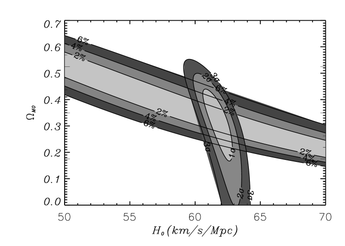
(b)

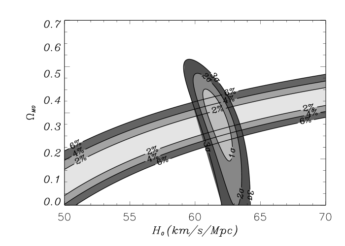
Figure 1: In panel (a) 1$\sigma$, 2$\sigma$ and 3$\sigma$ confidence limits (oval) for fits of luminosity distances of type Ia supernovae (SneIa) in the Riess06 gold dataset [12] are compared to parameters within the ($\Omega_{\lower 2.0pt\hbox{$\scriptstyle M0$}}$,$H_{\lower 2.0pt\hbox{$\scriptstyle 0$}}$) plane which fit the angular scale of the sound horizon $\delta=0.01$ rad deduced for WMAP [15], to within 2%, 4% and 6%. In panel (b) the SneIa are similarly compared to an effective comoving baryon acoustic oscillation (BAO) scale of $104h^{-1}$Mpc, as verified in galaxy clustering statistics [13]. The sound horizon angular scale and BAO comoving scale generally fit for different parameters, yet agree with each other for the same parameters that best fit the SneIa data, in a range that also agrees with the Hubble constant measurement of Sandage et al. [14]: $H_{\lower 2.0pt\hbox{$\scriptstyle 0$}}=62.3\pm 1.3\,\hbox{(stat)}\pm 5.0\,\hbox{(syst)}\,\hbox{km}\;\,\hbox{sec}^{-1}\,\hbox{Mpc}^{-1}$. We find $H_{\lower 2.0pt\hbox{$\scriptstyle 0$}}=61.7^{+1.2}_{-1.1}\,\hbox{km}\;\,\hbox{sec}^{-1}\,\hbox{Mpc}^{-1}$ and $\Omega_{\lower 2.0pt\hbox{$\scriptstyle M0$}}=0.33^{+0.11}_{-0.16}$ using $1\sigma$ statistical uncertainties from SneIa only. A 4% match to both sound horizon and BAO scales would reduce the bounds on $\Omega_{\lower 2.0pt\hbox{$\scriptstyle M0$}}$ by a factor of two. Note: $\Omega_{\lower 2.0pt\hbox{$\scriptstyle M0$}}$ is the “conventional dressed density parameter”[4]. Further details are provided in ref. [9].

References

References

- [1] G.F.R. Ellis, in B. Bertotti, F. de Felice and A. Pascolini (eds), General Relativity and Gravitation, (Reidel, Dordrecht, 1984) pp. 215–288.
- [2] L.B. Szabados, Living Rev. Rel. 7, 4 (2004).
- [3] T. Buchert, Gen. Relativ. Grav. 32, 105 (2000); Gen. Relativ. Grav. 33 (2001) 1381.
- [4] D.L. Wiltshire, New J. Phys. 9 (2007) 377.
- [5] A. Einstein and E.G. Straus, Rev. Mod. Phys. 17 (1945) 120; Err. ibid. 18 (1946) 148.
- [6] S. Jha, A.G. Riess and R.P. Kirshner, Astrophys. J. 659 (2007) 122.
- [7] W.M. Wood-Vasey et al., Astrophys. J. 666 (2007) 694.
- [8] D.L. Wiltshire, Phys. Rev. Lett. 99 (2007) 251101.
- [9] B.M. Leith, S.C.C. Ng and D.L. Wiltshire, Astrophys. J. 672 (2008) L91.
- [10] T. Buchert, Class. Quantum Grav. 22 (2005) L113; Class. Quantum Grav. 23 (2006) 817; M.N. Célérier, arXiv:astro-ph/0702416; and references therein.
- [11] A. Ishibashi and R.M. Wald, Class. Quantum Grav. 23 (2006) 235.
- [12] A.G. Riess et al., arXiv:astro-ph/0611572.
- [13] D.J. Eisenstein et al., Astrophys. J. 633 (2005) 560; S. Cole et al., Mon. Not. R. Astr. Soc. 362 (2005) 505.
- [14] A. Sandage, G.A. Tammann, A. Saha, B. Reindl, F.D. Macchetto and N. Panagia, Astrophys. J. 653 (2006) 843.
- [15] C.L. Bennett et al., Astrophys. J. Suppl. 148 (2003) 1; D.N. Spergel et al., arXiv:astro-ph/0603449.
- [16] G. Steigman, Int. J. Mod. Phys. E 15 (2006) 1; M. Asplund, D.L. Lambert, P.E. Nissen, F. Primas and V.V. Smith, Astrophys. J. 644 (2006) 229.
- [17] V.G. Gurzadyan, C.L. Bianco, A.L. Kashin, H. Kuloghlian and G. Yegorian, Phys. Lett. A 363 (2007) 121; V.G. Gurzadyan et al., Mod. Phys. Lett. A 20 (2005) 813.