Merging parton showers and matrix elements
— back to basics

Abstract:

We make a thorough comparison between different schemes of merging fixed-order tree-level matrix element generators with parton-shower models. We use the most basic benchmark of the $\mathcal{O}(\alpha_{S})$ correction to $e^{+}e^{-}\to\mbox{jets}$, where the simple kinematics allows us to study in detail the transition between the matrix-element and parton-shower regions. We find that the CKKW-based schemes give a reasonably smooth transition between these regions, although problems may occur if the parton shower used is not ordered in transverse momentum. However, the so-called Pseudo-Shower and MLM schemes turn out to have potentially serious problems due to different scale definitions in different regions of phase space, and due to sensitivity to the details in the initial conditions of the parton shower programs used.

1 Introduction

Accurate simulations of multi-jet final states are important for current experiments and will become even more so once the LHC starts. At the LHC the production rate for such states will be large due to the huge available phase space. Hadronic multi-jet states are used for many of the discovery channels for new physics and the main irreducible background comes from QCD. A good theoretical understanding and accurate physics simulations of multi-jet QCD states are therefore essential tools for understanding and analyzing LHC data.

To be able to compare the predictions of a model with a collider experiment, a description of final state hadrons is needed. There are a few phenomenological models available to describe the production of hadrons, but they all require that the perturbative emissions are well described, especially in the soft and collinear regions, to give reliable results. These collinear and soft emissions dominate the multi-parton cross section and can be taken into account to all orders, if one approximates the emissions to be strongly ordered, as is done in parton shower models. However, when the strong ordering no longer holds, which is the case if we have several hard and widely separated jets, the parton shower models become unreliable.

In order to improve the description of multi-jet states, full matrix elements can be used. These describe the process correctly up to a given order in the strong coupling constant. However, the matrix elements become difficult to calculate for high parton multiplicities or if one goes beyond tree-level. They also contain divergences in the soft and collinear limits and need to be regulated using cutoffs.

The idea behind merging algorithms is to let the matrix elements describe the hard emissions and use the parton shower to describe the soft and collinear emissions. To accommodate this, the phase space needs to be split into two well defined regions, one where emissions are generated by tree-level matrix elements, and one where emissions are generated by the parton shower. To avoid double counting and dead regions, the two regions should have no overlaps and together cover the entire phase space. The scale that describes the border between the regions is called the merging scale.

Some extra care is needed to avoid an artificial dependence on the merging scale. The matrix elements contain divergences in the soft and collinear regions, whereas the emission probability in these regions in the parton shower is finite since it is regulated by Sudakov form factors. The effects of the Sudakov form factors need to be included in the matrix element part of the phase space as well, making the state from the matrix element exclusive. Also a running coupling similar to that of the shower needs to be introduced. If this is done correctly the dependence on the merging scale should be minimal, however, especially for corrections with several extra jets, a small residual dependence on the merging scale from sub-leading terms is basically unavoidable.

There are four main algorithms that address the problem of merging tree-level matrix elements and partons showers: CKKW [1], CKKW-L [2], Pseudo-Shower [3], and MLM [4]. CKKW was first published for $e^{+}e^{-}$ collisions [1] and later extended to hadron collisions [5]. Implementations have been made in S HERPA [6] and in HERWIG [3, 7]. CKKW has been used in several studies of vector boson production in hadronic collisions [3, 8, 9, 10, 11]. CKKW-L was also first published for $e^{+}e^{-}$ [2] and later extended to hadrons and applied to $W$-production [12, 11]. All the CKKW-L results so far have been calculated using the A RIADNE [13] implementation. The Pseudo-Shower scheme was published in [3], where the algorithm was described, and an implementation based on P YTHIA [14] was applied to both $e^{+}e^{-}$ and hadron collisions. The MLM algorithm has been implemented in A LPGEN [15], M AD E VENT [16] and H ELAC [17]. There is also one implementation based on HERWIG and M AD E VENT , which was used in [3]. Several studies using MLM have been performed for heavy quark and vector boson production with incoming hadrons[3, 18, 19, 11]. To our knowledge no calculation applying MLM to $e^{+}e^{-}$ annihilation has been published.

Of all the implementations, only the S HERPA implementation of the CKKW scheme and the A LPGEN and M AD E VENT implementations of MLM are publicly available, while the others are obtainable from their respective authours upon request.

There have been some assessments of the systematics of the various algorithms done already, but the main focus so far has been the case of hadron collisions. Although collisions with incoming hadrons clearly are the most interesting in light of the upcoming LHC experiments, they also include a lot of complications, such as uncertainties from PDFs and BFKL-like corrections, that obfuscate the basic properties of the merging algorithms. $e^{+}e^{-}$ annihilation is much simpler from a theoretical point of view and is therefore more suitable for testing the basic properties of the different algorithms. We believe it is essential to test the algorithms for $e^{+}e^{-}$ annihilation before moving on to hadron collisions.

Systematics for $e^{+}e^{-}$ have been published for CKKW-L [2] and for CKKW and Pseudo-Shower [3], but the systematics for the Pseudo-Shower approach was quite limited. These studies are extended in this paper, where the four algorithms listed earlier are applied to different parton shower implementations. This allows us to thoroughly test which algorithms live up to their promises.

To study systematics with as little complications as possible we only look at the simple case of $e^{+}e^{-}\rightarrow q\bar{q}g$. In this case the matrix element correction is already implemented in most of the parton showers, using a simple reweighting of the hardest splitting[20, 21, 22, 23], which makes this process particularly suitable for testing the various algorithms. Ideally all the calculations should show small deviations and yield more or less trivial results. However, we find that this is not the case.

Since the process studied is rather simple, algorithms that perform well should also be tested with more complicated processes before they can be reliably used to predict experimental observables. Some of the complications that can occur during the merging do not enter if only first order corrections are applied. However, if an algorithm does not perform well for this simple process, it is improbable that it will work reliably for more complicated processes.

We note that besides the four merging algorithms presented here, there are also other ways of combining matrix elements and parton showers, e.g. the methods based on modifyig the tree-level or NLO matrix elements to match the parton shower (see e.g. [24, 25, 26, 27, 28, 29, 30, 31, 32]). Such matching algorithms may also have a dependence on an artificial matching scale. Although it may be interesting to also benchmark these algorithms using the simplest $e^{+}e^{-}\to qg\bar{q}$ process, we have not done so in this paper.

In this paper we will concentrate on the behavior of the merging schemes in absolute numbers. It would also be interesting to study their formal properties in terms of leading double- and single-logarithmic contributions to various cross sections, which so far has only been done for the CKKW scheme[1]. We plan to return to such issues in a future publication.

In this article we start by reviewing the theoretical aspects of the four algorithms in section 2. Then we move on to showing results from our implementations of the algorithms in section 3 and finally in section 4 we present our conclusions.

2 Theory

All of the algorithms considered in this paper aim to do a good job of merging matrix elements and partons showers. The issues that are addressed are the same, namely to split the phase space in a clean well defined way and to make the matrix element event exclusive by introducing Sudakov form factors or using some other similar suppression. The main aim is to minimize any artificial dependence on the merging scale.

2.1 General Scheme

The basic steps are common to all the algorithms and can be summarized as follows:

1. Select a process to be studied and choose a scheme to cutoff the divergences in the matrix elements, typically using a jet measure. Specify the maximum parton multiplicity to be generated by the matrix elements (This is currently limited to five or six extra partons for computational reasons). Calculate the cross section for all the parton multiplicities.

2. Select a parton multiplicity with a probability proportional to its integrated cross section. Generate kinematics according to the matrix element.

3. Calculate a weight for the event based on the Sudakov form factors and the running coupling. Use this weight either to reweight the event or as a probability for rejecting the event. If the event is rejected generate a new event according to step 2.

4. Find a set of initial conditions for the parton shower and invoke the shower. This may include a veto on the emissions from the shower.

All the algorithms considered in this paper do steps 1 and 2 in the same way, but steps 3 and 4 are done using rather different approaches. Each algorithm has its own way of including the Sudakov form factors and finding a good set of initial conditions for the shower.

One of the key features that distinguishes the algorithms is the choice of scales. The algorithms uses different definitions of scales when determining how to split phase space between the matrix element and the parton shower and in calculating the Sudakov form factors. Furthermore, these scale definitions may be different from what determines the ordering of emissions in the parton showers. We show later in this paper that the scale choices have significant consequences for how well the dependence on the merging scale can be minimized.

The rest of this section describes the details of each algorithm and their consequences for the physics result. The descriptions of the algorithms are limited to $e^{+}e^{-}$ collisions, but, with a few modifications and extensions, they have all been used to calculate results for hadron collisions.

2.2 CKKW

The theoretical foundation for CKKW was published in [1], but the main points are repeated here for completeness. CKKW is focuses on the Durham $k_{\perp}$-algorithm for clustering jets in $e^{+}e^{-}$ [35], where the distance between two partons, $i$ and $j$, is defined as

$$y_{ij}\equiv 2\min(E_{i}^{2},E_{j}^{2})(1-cos\theta_{ij})/E_{\mathrm{CM}}^{2}.$$ (1)

The $k_{\perp}$-algorithm is used to construct a parton shower history from the event generated according to the matrix element. The algorithm generates a set of clusterings and corresponding scales, which are later used to calculate the Sudakov form factors and the running coupling.

Before going through the CKKW algorithm some notation needs to be introduced. $\Gamma_{q}$, $\Gamma_{g}$ and $\Gamma_{f}$ are the branching probabilities for $q\rightarrow qg$, $g\rightarrow gg$ and $g\rightarrow f\bar{f}$ respectively. The Sudakov form factors are then given by

$$\Delta_{q}(Q_{1},Q_{2}) = \exp(-\int_{Q_{2}}^{Q_{1}}dq\Gamma_{q}(Q_{1},q))$$ (2)

$$\Delta_{g}(Q_{1},Q_{2}) = \exp(-\int_{Q_{2}}^{Q_{1}}dq(\Gamma_{g}(Q_{1},q)+\Gamma_{f}(Q_{1},q))).$$ (3)

They can be interpreted as the probability of a parton with the production scale $Q_{1}$ not to have a branching above the scale $Q_{2}$. Note the dependency on the production scale in the branching probabilities. This means that the Sudakov form factors used in CKKW do not factorize ($\Delta(Q_{1},Q_{2})\cdot\Delta(Q_{2},Q_{3})\neq\Delta(Q_{1},Q_{3})$). This is also the case for the Sudakov form factors in the angular ordered shower, where the limits on the integration of the splitting functions are dependent on the production scale.

The idea of CKKW is to use the full matrix element for the branching probabilities and analytical Sudakov form factors above the merging scale, and the parton shower below the merging scale. The full CKKW algorithm is the following:

1. Calculate cross sections and generate events according to step 1 and 2 in section 2.1. $y_{\mathrm{MS}}$ denotes the merging scale which is equal to the matrix element cutoff, defined in terms of the $k_{\perp}$-measure in eq. (1). The events are generated using a fixed strong coupling, $\alpha_{\mathrm{sME}}$, and a maximum multiplicity, $N$.

2. Construct a shower history by applying the $k_{\perp}$-algorithm to the state from the matrix element. The algorithm is constrained to only allow clusterings of partons which are consistent with a possible emission from the parton shower. This yields a set of clustering values $y_{2},...,y_{n}$, where $y_{2}=1>y_{3}>...>y_{n}$ and $n$ denotes the parton multiplicity of the event from the matrix element. Use the result from the clustering to determine a set of nodes where the partons are merged and the associated scales, $q_{i}^{2}=y_{i}E_{\mathrm{CM}}^{2}$.

3. Calculate a weight for the running coupling given by $\prod_{i=3}^{n}\alpha_{s}(q_{i})/\alpha_{\mathrm{sME}}^{n-2}$.

4. For each internal line of type $i$ running between a node with scale $q_{j}$ and $q_{k}$ apply a factor $\Delta_{i}(q_{j},q_{\mathrm{MS}})/\Delta_{i}(q_{k},q_{\mathrm{MS}})$, where $q_{\mathrm{MS}}^{2}=y_{\mathrm{MS}}E_{\mathrm{CM}}^{2}$. For external lines of type $i$ starting from a scale $q_{j}$ apply the weight $\Delta_{i}(q_{j},q_{\mathrm{MS}})$. These weights are the Sudakov form factors and they are calculated analytically.

5. Reweight the event with the product of the Sudakov form factors in step 4 and the running coupling weight in step 3.

6. Set the starting scale of each parton to the scale associated with the node in the shower history where it was produced. Invoke the shower and veto any emission which would give a $k_{\perp}$-measure above $y_{\mathrm{MS}}$.

The original CKKW procedure[1] contained no special treatment for highest multiplicity events. This needs to be included since applying the veto on emissions in the shower down to the merging scale would prevent events with more than $N$ jets above the merging scale from being generated. One way to resolve this is to modify the procedure for highest multiplicity events ($n=N$) and use the scale $q_{n}$ instead of $q_{\mathrm{MS}}$ in the Sudakov form factors and the vetoed shower. This is done in [3, 36].

Another issue that needs to be addressed is effects related to the choice of ordering variable in the shower. The entire theoretical derivation in the CKKW publication[1] uses only one way of defining scales, namely the Durham $k_{\perp}$. While the discrepancy from using a different ordering variable in the shower may cancel to some accuracy, this is not explicitly shown or discussed, even though the shower used in the publication is ordered in virtuality. The consequences of applying the scheme to a shower not ordered in Durham $k_{\perp}$ are therfore somewhat unclear.

The original CKKW publication[1] claims that this procedure cancels the dependence on the merging scale to next-to-leading logarithmic (NLL) accuracy. However, this claim assumes that the formalism used, including Sudakov form factors, jet rates and generating functions, is valid at NLL, but this proof has never been published.

2.3 CKKW-L

The CKKW-L algorithm goes through the same basic steps as CKKW, but has a different way of calculating the Sudakov form factors and implementing the veto in the shower. In the CKKW-L scheme, a full cascade history with intermediate states is constructed. What is done is basically to run the cascade backwards and answer the question “how could the shower have generated this state?”. This means that the ordering scale in the shower is used when clustering the partons. As in the CKKW case, only physically allowed clusterings are considered. However, contrary to CKKW where always the smallest scale is chosen for each clustering, all possible ordered shower histories are considered, and one is chosen according to a probability proportional to the product of the relevant branching probabilities. The chosen shower history is then used to calculate the Sudakov form factors and the running coupling.

To be able to use this scheme, the parton shower needs to have well defined intermediate states and it is also required that the Sudakov form factors factorize ($\Delta(Q_{1},Q_{2})\cdot\Delta(Q_{2},Q_{3})=\Delta(Q_{1},Q_{3})$). This is achieved if the Sudakov form factors only depend on the kinematics of the intermediate state rather than the production scale. This is for example the case in the dipole shower used in A RIADNE [13] and the $p_{\perp}$-ordered shower in P YTHIA [37], but not for the angular ordered shower in HERWIG [7].

The effects of the running coupling are taken into account by reweighting with the same $\alpha_{\mathrm{s}}$ as in the shower with the constructed scales as input. The Sudakov form factors are introduced by using the shower to generate single emissions from the constructed states starting from the constructed scales and rejecting the event if the emission is above the next constructed scale. This is known as the Sudakov veto algorithm and it is equivalent to accepting events with a probability equal to the Sudakov form factor, since by definition the no emission probability of the shower is equal to the Sudakov form factor.

There are several advantages to this approach. One is that it makes sure that the Sudakov form factors above and below the merging scale match exactly and another is that any corrections introduced in the shower is also included in the Sudakov form factor. This is particularly useful if the splitting functions have been reweighted with matrix elements, since this makes it possible to completely cancel the merging scale dependence for first order correction (shown explicitly below). We also expect that the cancellation of the first order correction will lead to a smaller merging scale dependence for higher order processes even though the complete cancellation no longer holds.

We use a slightly different notation in this section to emphasize the difference in the Sudakov form factors with respect to the ones in CKKW. $\Delta_{S_{n}}(\rho_{1},\rho_{2})$ denotes a Sudakov form factor for an $n$-particle state giving the probability that there is no emission with a shower scale, $\rho$, between $\rho_{1}$ and $\rho_{2}$. The merging scale uses another notation, $Q_{\mathrm{MS}}$, to emphasize that this scale does not need to be defined in terms of the emission scale in the shower. In fact, one could in principle use any partonic scale definition for the merging scale. These are the steps in the CKKW-L algorithm.

1. Calculate cross sections and generate events according to step 1 and 2 in section 2.1. $Q_{\mathrm{MS}}$ denotes the merging scale which is equal to the matrix element cutoff and may be defined using any choice of scale. The events are generated using a fixed strong coupling, $\alpha_{\mathrm{sME}}$, and a maximum parton multiplicity, $N$.

2. Construct a full cascade history by considering all possible ordered histories and selecting one randomly with a probability proportional to the product of the branching probabilities. If no ordered histories can be constructed, unordered ones are considered. This results in a set of intermediate states ($S_{2},S_{3},...S_{n}$) and scales ($\rho_{2}=\rho_{\mathrm{max}},\rho_{3},...,\rho_{n}$). $S_{2}$ denotes here denotes the constructed $2\rightarrow 2$ process and $S_{n}$ is the state given by the matrix element. $n$ is the parton multiplicity in the event, $\rho_{\mathrm{max}}$ is the maximum scale of the process and $\rho_{i}$ is the constructed scale where the state $S_{i-1}$ emits a parton to produce the state $S_{i}$.

3. Reweight the events with $\prod_{i=3}^{n}\alpha_{s}(\rho_{i})/\alpha_{\mathrm{sME}}^{n-2}$.

4. For each state $S_{i}$ (except $S_{n}$), generate an emission with $\rho_{i}$ as starting scale and if this emission occurred at a scale larger than $\rho_{i+1}$ reject the event. This is equivalent to reweighting with a factor $\prod_{i=2}^{n-1}\Delta_{S_{i}}(\rho_{i},\rho_{i+1})$.

5. For the last step there are two cases.

   • If the event does not have the highest multiplicity $n<N$, generate an emission from the state $S_{n}$ with $\rho_{n}$ as starting scale. If the emission is above the merging scale $Q_{\mathrm{MS}}$, reject the event. Otherwise accept the event and continue the cascade.

   • If the event has the highest possible multiplicity $n=N$, accept the event and start the cascade from the state $S_{n}$ with the scale $\rho_{n}$.

The algorithm introduces all the factors that would have been present if the event had been generated by the parton shower, except the branching probability which is taken from the matrix element. To show how this comes about, a derivation of the parton multiplicity cross sections for a first order matrix element is shown below. The explicit reweighting of $\alpha_{\mathrm{s}}$ is not shown, but is straight forward to include.

Let $\rho_{0}$ denote the parton shower cutoff and $\Gamma_{S_{n}}(\rho)$ denote the probability that a state $S_{n}$ branches at scale $\rho$. The definition of the Sudakov from factor in this case is $\Delta_{S_{n}}(\rho_{1},\rho_{2})\equiv\exp(-\int_{\rho_{2}}^{\rho_{1}}d\rho\,\Gamma_{S_{n}}(\rho))$. The exclusive parton multiplicity cross sections generated by the standard parton shower can be written as

$$\sigma^{\mathrm{PS}}_{2}(\rho_{\mathrm{max}},\rho_{0}) = \sigma_{0}\,\Delta_{S_{2}}(\rho_{\mathrm{max}},\rho_{0})$$ (4)

$$\sigma^{\mathrm{PS}}_{3}(\rho_{\mathrm{max}},\rho_{0}) = \sigma_{0}\int_{\rho_{0}}^{\rho_{\mathrm{max}}}d\rho\,\Delta_{S_{2}}(\rho_{\mathrm{max}},\rho)\,\Gamma_{S_{2}}(\rho)\,\Delta_{S_{3}}(\rho,\rho_{0})$$ (5)

$$\sigma^{\mathrm{PS}}_{4}(\rho_{\mathrm{max}},\rho_{0}) = \sigma_{0}\int_{\rho_{0}}^{\rho_{\mathrm{max}}}d\rho\,\Delta_{S_{2}}(\rho_{\mathrm{max}},\rho)\,\Gamma_{S_{2}}(\rho)\times$$ (6)

$$\times\int_{\rho_{0}}^{\rho}d\rho^{\prime}\,\Delta_{S_{3}}(\rho,\rho^{\prime})\,\Gamma_{S_{3}}(\rho^{\prime})\,\Delta_{S_{4}}(\rho^{\prime},\rho_{0}).$$

This notation can be generalized to include all higher multiplicity cross sections. Let $f^{{3}\shortrightarrow{n}}(\rho,\rho_{0})$ denote the probability of the three-parton state to evolve into an $n$ parton state between the two given scales. This means that a general $n\geq 3$ parton cross section can be written as

$$\sigma^{\mathrm{PS}}_{n}(\rho_{\mathrm{max}},\rho_{0}) = \sigma_{0}\int_{\rho_{0}}^{\rho_{\mathrm{max}}}d\rho\,\Delta_{S_{2}}(\rho_{\mathrm{max}},\rho)\,\Gamma_{S_{2}}(\rho)f^{{3}\shortrightarrow{n}}(\rho,\rho_{0}),$$ (7)

where

$$f^{{3}\shortrightarrow{3}}(\rho,\rho_{0}) = \Delta_{S_{3}}(\rho,\rho_{0}).$$ (8)

$$f^{{3}\shortrightarrow{4}}(\rho,\rho_{0}) = \int_{\rho_{0}}^{\rho}d\rho^{\prime}\,\Delta_{S_{3}}(\rho,\rho^{\prime})\,\Gamma_{S_{3}}(\rho^{\prime})\,\Delta_{S_{4}}(\rho^{\prime},\rho_{0})$$ (9)

$$\vdots$$

The merging scale may be defined using a different way of mapping the phase space (denoted $Q$) as compared to the scale used in the shower. The value of the scale used to define the merging scale and the scale of the shower can be related if the other variables that determine the shower emission is included. Let $\vec{x}$ represent the $k$ additional variables used in the shower, which may include energy fractions and rotation angles. The branching probability can be written in a way that it includes the dependence on these variables as long as the following is true.

$$\Gamma(\rho)=\int d^{k}\vec{x}\,\Gamma(\rho,\vec{x})$$ (10)

The alternative mapping of phase space is described by the function $Q_{S_{n}}(\rho,\vec{x})$, which denotes the value of the merging scale measure for a given shower emission. The lowest order matrix element cross sections are equal to

$$\sigma^{\mathrm{ME}}_{2}(\rho_{\mathrm{max}},Q_{\mathrm{MS}}) = \sigma_{0}$$ (11)

$$\sigma^{\mathrm{ME}}_{3}(\rho_{\mathrm{max}},Q_{\mathrm{MS}}) = \sigma_{0}\int_{\rho_{0}}^{\rho_{\mathrm{max}}}d\rho\int d^{k}\vec{x}\,\Theta(Q_{S_{2}}(\rho,\vec{x})-Q_{\mathrm{MS}})\,\Gamma^{\mathrm{ME}}_{S_{2}}(\rho,\vec{x}).$$ (12)

$\Gamma^{\mathrm{ME}}_{S_{2}}$ is the branching probability in the matrix element and $\Theta$ is the standard Heaviside function. Note that the equations above only hold if the matrix element merging scale is above the shower cutoff everywhere in phase space, but this can be resolved by discarding all events from the matrix element which are below the shower cutoff.

The next step is to apply the algorithm to calculate the jet rates at $\rho_{0}$ for the merged matrix element and parton shower. The two-jet state is already the lowest order process, which means no cascade history is constructed and only the final Sudakov veto down to the merging scale enters. The parton multiplicity cross sections become equal to that of the pure shower minus the cross section for events with the first emission above $Q_{\mathrm{MS}}$. The two-jet matrix-element contributions to the cross sections are equal to

$$\sigma_{2}(\rho_{\mathrm{max}},\rho_{0}) = \sigma_{0}\,\Delta_{S_{2}}(\rho_{\mathrm{max}},\rho_{0})$$ (13)

$$\sigma_{n}(\rho_{\mathrm{max}},\rho_{0}) = \sigma_{0}\int_{\rho_{0}}^{\rho_{\mathrm{max}}}d\rho\int d^{k}\vec{x}\,\Theta(Q_{\mathrm{MS}}-Q_{S_{2}}(\rho,\vec{x}))\,\Delta_{S_{2}}(\rho_{\mathrm{max}},\rho)\times$$ (14)

$$\times\Gamma_{S_{2}}(\rho,\vec{x})f^{{3}\shortrightarrow{n}}(\rho,\rho_{0}).$$

When the algorithm is applied to a three-jet event, an emission scale, $\rho_{3}$, is constructed. Emissions are generated from the two-jet state and events discarded according to the Sudakov veto algorithm, which is equivalent to introducing a weight $\Delta_{S_{2}}(\rho_{\mathrm{max}},\rho_{3})$. The cascade is then started from the scale $\rho_{3}$ and, assuming the three-jet configuration is the highest multiplicity, no additional Sudakov suppression is included. Using the matrix element cross section from equation (12) and, assuming that the constructed scale $\rho_{3}$ is equal to the scale used in the matrix element, results in the following contributions to the parton multiplicity cross sections.

$$\sigma_{n}(\rho_{\mathrm{max}},\rho_{0}) = \sigma^{\mathrm{ME}}_{3}(\rho_{\mathrm{max}},Q_{\mathrm{MS}})\,\Delta_{S_{2}}(\rho_{\mathrm{max}},\rho_{3})\,f^{{3}\shortrightarrow{n}}(\rho_{3},\rho_{0})=$$ (15)

$$= \sigma_{0}\int_{\rho_{0}}^{\rho_{\mathrm{max}}}d\rho\int d^{k}\vec{x}\,\Theta(Q_{S_{2}}(\rho,\vec{x})-Q_{\mathrm{MS}})\,\Gamma^{\mathrm{ME}}_{S_{2}}(\rho,\vec{x})\times$$

$$\times\Delta_{S_{2}}(\rho_{\mathrm{max}},\rho)\,f^{{3}\shortrightarrow{n}}(\rho,\rho_{0})$$

The following cross sections are the result from adding the contributions from the two- and three-jet processes.

$$\sigma^{\mathrm{ME+PS}}_{2}(\rho_{\mathrm{max}},\rho_{0}) = \sigma_{0}\,\Delta_{S_{2}}(\rho_{\mathrm{max}},\rho_{0})$$ (16)

$$\sigma^{\mathrm{ME+PS}}_{n}(\rho_{\mathrm{max}},\rho_{0}) = \sigma_{0}\,\int_{\rho_{0}}^{\rho_{\mathrm{max}}}d\rho\int d^{k}\vec{x}\,[\Gamma^{\mathrm{ME}}_{S_{2}}(\rho,\vec{x})\,\Theta(Q_{S_{2}}(\rho,\vec{x})-Q_{\mathrm{MS}})+$$ (17)

$$+\Gamma^{\mathrm{PS}}_{S_{2}}(\rho,\vec{x})\Theta(Q_{\mathrm{MS}}-Q_{S_{2}}(\rho,\vec{x}))]\,\Delta_{S_{2}}(\rho_{\mathrm{max}},\rho)\,f^{{3}\shortrightarrow{n}}(\rho,\rho_{0})$$

From the equations above one can see that the only dependence on the merging scale $Q_{\mathrm{MS}}$ is in the integration over the branching probabilities. This means that the merging scale dependence for this process cancels to the accuracy of which the shower generates the first emission. In fact, for the process studied in this paper, many of the parton shower implementations reweight the splitting function for the first emission with the matrix element, in which case the merging scale dependence cancels completely.

2.4 Pseudo-Shower

The Pseudo-Shower algorithm is similar in spirit to CKKW-L, but it uses partonic jet observables for the kinematics instead of individual partons. Where CKKW-L runs the cascade one emission at a time from a given parton state to calculate no-emission probabilities, in the Pseudo-Shower approach a full parton cascade is evolved, and the resulting partons are clustered back to jets. Any standard clustering algorithm, where in each step the pair of particles which are closest together are clustered, can be used. The same distance measure is used to define the merging scale as the one used to construct a shower history for the matrix-element state and the fully showered states. The full algorithm is defined as follows.

1. Choose a jet clustering scheme to be used in the algorithm and a merging scale, $d_{\mathrm{MS}}$. Set the matrix element cutoff equal to the merging scale, calculate cross sections and generate events according to step 1 and 2 in section 2.1. The events are generated using a fixed strong coupling, $\alpha_{\mathrm{sME}}$, and a maximum multiplicity, $N$.

2. Cluster the partons from the matrix element, using the selected jet scheme, until a $2\rightarrow 2$ state is reached. As in CKKW, only clusterings corresponding to physically allowed splittings are considered. The result of the clustering is interpreted as a shower history with a set of states ($S_{2},\ldots S_{n}$) and a set of scales ($\tilde{d}_{2}=d_{\mathrm{max}},\tilde{d}_{3},\ldots,\tilde{d}_{n}$), where $n$ is the parton multiplicity of the event.

3. For each state $S_{i}$, except $S_{n}$, perform a full shower vetoing any emission with a jet measure greater than the corresponding scale in the shower history, $d>\tilde{d}_{i}$. Calculate a set of clustering scales, $d_{j}$, by clustering the partons from the shower using the same algorithm as in step 2, but for practical reasons also allow clusterings corresponding to non-physical splittings. Reject the event if $\sqrt{d_{i+1}}>\sqrt{\tilde{d}_{i+1}}+\delta$ (the $\delta$ is a fudge factor to be discussed below).

4. For the final state $S_{n}$ the shower is invoked, vetoing emissions with $d>\tilde{d}_{n}$. If the event is not a maximum multiplicity event ($n<N$), the partons are clustered and the event is rejected if the scale from the clustering is above the merging scale, $\sqrt{d_{n+1}}>\sqrt{d_{\mathrm{MS}}}+\delta$. For $N=n$ the event is accepted except if $\sqrt{d_{n+1}}>\sqrt{\tilde{d}_{n}}+\delta$.

Although it was not stated in the text in [3], the implementation did include a reweighting with a running strong coupling $\prod_{i=3}^{n}\alpha_{\mathrm{s}}(\tilde{d}_{i})/\alpha_{\mathrm{sME}}^{n-2}$. The same reweighting is also included here.

To see the similarity with CKKW-L, consider using the Pseudo-Shower using a parton shower with an ordering variable equal to the distance scale in the clustering algorithm used, and with well-defined intermediate states. In the strongly ordered limit, the clustering algorithm would then exactly reproduce the intermediate states and branching scales in the shower. This means that evolving a full shower from the state $S_{i}$, starting from a scale $\tilde{d}_{i}$, clustering to find a $d_{i+1}$ and rejecting the event if $d_{i+1}>\tilde{d}_{i+1}$ would exactly correspond to the Sudakov form factor $\Delta_{S_{i}}(\tilde{d}_{i},\tilde{d}_{i+1})$, and the merging scale dependence for first order matrix element corrections would cancel in the same way as CKKW-L.

In reality, the clustering does not exactly reconstruct the shower splittings. If subsequent emissions are not clustered in the same way as the shower emitted them, this can affect the clustering scale of harder emissions. This means that the scale of the matrix element partons before the shower and the scale that one gets from the jet clustering after the shower are rarely the same. This is a significant problem, since the phase space cuts that separate the matrix element emissions from the partons shower emission is done using two different scales, which leads to dead regions and double counting of emissions and it also affects the calculation of the Sudakov form factors.

To moderate the effects of having two different scales, the fudge factor $\delta$ (introduced in [3]) was included whenever comparing a scale from the clustering of the matrix element state with a scale from the clustering of the fully showered state. In [3] the value $\delta=2$ GeV was used without motivation, theoretical or otherwise, but supposedly the parameter needs to be tuned for each choice of process and merging scale to properly compensate for the mismatch in scales.

2.5 MLM

The MLM algorithm is similar to the Pseudo-Shower in that it also does matching with partonic jet observables. The algorithm is much simpler to implement compared to earlier schemes discussed. In the MLM merging scheme the event from the matrix element is simply fed into the parton shower program, the shower is invoked and the final state partons are clustered into jets. The algorithm then specifies that the matrix element partons should be matched to the final state partonic jets, and events are accepted only if all the jets match and the event contains no extra jets above the merging scale. In this way the Sudakov form factors are approximated by the probability that there are no emissions above the merging scale and, at the same time, the parton shower emissions are approximately constrained to be below the merging scale. The MLM algorithm is a really convenient way of doing merging since it requires no modifications to the parton shower program.

Even though MLM has been frequently used, a general version of the algorithm has never been published and all the published algorithms assume incoming hadrons. Based on [4, 11, 19], we present here our interpretation of the necessary steps needed for applying the MLM scheme to $e^{+}e^{-}$ collisions.

The first step in an MLM implementation is to choose a jet definition to be used for the merging scale and the matrix element cutoff. The original MLM algorithm used cone jet definitions, although there have been implementations using the $k_{\perp}$-algorithm, e.g. the M AD E VENT implementation in [11] and the HERWIG implementation in [3]. After specifying a cutoff, events are generated and the running coupling reweighting is calculated in the same way as in the CKKW algorithm.

Then the shower is invoked using an appropriate starting scale, which is defined for each implementations and process. For $W$-production in hadron collisions, the scale is set to the transverse mass of the $W$ ($\sqrt{m_{W}^{2}+p_{\perp W}^{2}}$)[11], whereas for the top production implementation it is not specified [19]. In hadron collision there is some freedom for choosing the starting scale of the shower, but for $e^{+}e^{-}$ we think that the scale should be set to center of mass energy, to allow the shower to utilize the full phase space.

After the shower has been invoked the final state partons need to be clustered into jets and matched to the partons from the matrix element. The clustering is done with the same algorithms used to define the merging scale. The partons from the matrix element are then matched to the clustered jets, in order of decreasing energy. The measure used to match the partons to jets is some quantity related to the jet clustering. These are all the steps in the algorithm.

1. Select a merging scale, $Q_{\mathrm{MS}}$, and a matrix element cutoff $Q_{\mathrm{cut}}$, such that $Q_{\mathrm{cut}}<Q_{\mathrm{MS}}$, where the scales are defined using a jet algorithm. Calculate cross sections and generate events according to step 1 and 2 in section 2.1. The events are generated using a fixed strong coupling, $\alpha_{\mathrm{sME}}$, and a maximum parton multiplicity, $N$.

2. Cluster the partons from the matrix element using the $k_{\perp}$-algorithm and use the clustering scales as in input to $\alpha_{\mathrm{s}}$ and reweight the event.

3. Feed the event into a parton shower using the Les Houches interface[38], setting the scale to $E_{\mathrm{CM}}$, and start the shower.

4. Cluster the partons to jets using the algorithm from step 1 with a clustering scale set to $Q_{\mathrm{MS}}$. Go through the list of partons, in order of decreasing energy, and match them to the clustered jets. This is done by finding the jet with the smallest distance to the parton defined using some measure based on the jet clustering scheme. If not all the partons match or there are extra jets, reject the event.

   For the highest multiplicity events either use a higher clustering scale and more relaxed matching criteria or allow extra jets that are softer than the matched jets.

There are several aspects of this algorithm that needs further explaining. The reason for having a cutoff below the merging scale is that events slightly below the merging scale can end up above after the shower. This leaves an arbitrary choice of matrix element cutoff, but this can be resolved if soft and collinear particles have a vanishing probability to generate an independent jet, which means that the result converge when the matrix element cutoff is lowered. This is a way of getting around the problem that occurred in the Pseudo-Shower algorithm, namely that the cuts on the matrix element state and on the partonic jets are not equivalent. However, the convergence needs to be verified for each implementation and process.

One other aspect that needs further scrutiny is what happens inside the parton shower program. The main danger is that the program may be given a state with one or more relatively soft parton and a rather high starting scale, which means that the shower often ends up emitting harder partons than the ones already present, leading to an unordered shower. This breaks the strong ordering approximation, which is fundamental to all parton showers, and the end result is heavily dependent on how unordered emissions are handled.

To derive some of the properties of MLM, let us assume (as we did in the Pseudo-Shower case) that the jet clustering is a perfect inverse of the shower and that the shower has well defined intermediate states. These assumptions are a bit crude considering the way MLM is used in current implementations, but it allows for the possibility to do analytical calculations and it should give some idea of what to expect from the algorithm. Under these assumptions parton multiplicity cross sections, including the first order matrix element corrections, can be calculated.

The calculations are performed using the same notation as in the section 2.3. The merging scale can be defined in terms of the scale in the shower ($\rho_{\mathrm{MS}}$) and starting the scale from the center of mass energy is equivalent to using the maximum scale ($\rho_{\mathrm{max}}$). The two-jet matrix element contribution to the parton multiplicity cross sections becomes the same as in CKKW-L.

$$\sigma_{2}(\rho_{\mathrm{max}},\rho_{0}) = \sigma_{0}\cdot\Delta_{S_{2}}(\rho_{\mathrm{max}},\rho_{0})$$ (18)

$$\sigma_{n}(\rho_{\mathrm{max}},\rho_{0}) = \sigma_{0}\cdot\int_{\rho_{0}}^{\rho_{\mathrm{MS}}}d\rho\,\Delta_{S_{2}}(\rho_{\mathrm{max}},\rho)\,\Gamma_{S_{2}}(\rho)f^{{3}\shortrightarrow{n}}(\rho,\rho_{0})$$ (19)

The contribution from the three-jet is different however. The reason is that there is no Sudakov form factor from a two-particle state included since no shower history was considered. The contribution to the cross sections is the following.

$$\sigma_{n}(\rho_{\mathrm{max}},\rho_{0}) = \sigma_{0}\cdot\int_{\rho_{\mathrm{MS}}}^{\rho_{\mathrm{max}}}d\rho\,\Gamma^{\mathrm{ME}}_{S_{2}}(\rho)\,\Delta_{S_{3}}(\rho_{\mathrm{max}},\rho)\,f^{{3}\shortrightarrow{n}}(\rho,\rho_{0})$$ (20)

The sum of the two contributions become the following.

$$\sigma_{2}(\rho_{\mathrm{max}},\rho_{0}) = \sigma_{0}\cdot\Delta_{S_{2}}(\rho_{\mathrm{max}},\rho_{0})$$ (21)

$$\sigma_{n}(\rho_{\mathrm{max}},\rho_{0}) = \sigma_{0}\cdot\int_{\rho_{0}}^{\rho_{\mathrm{max}}}d\rho\,\left[\Gamma^{\mathrm{ME}}_{S_{2}}(\rho)\,\Delta_{S_{3}}(\rho_{\mathrm{max}},\rho)\Theta(\rho-\rho_{\mathrm{MS}})+\right.$$ (22)

$$\left.+\Gamma^{\mathrm{PS}}_{S_{2}}(\rho)\,\Delta_{S_{2}}(\rho_{\mathrm{max}},\rho)\Theta(\rho_{\mathrm{MS}}-\rho)\right]f^{{3}\shortrightarrow{n}}(\rho,\rho_{0})$$

Comparing equation (21) to (4) one can see that the two-parton cross section becomes the correct one. Note that this would not have be the case if a lower starting scale was chosen for the shower. The higher multiplicity cross sections contain complications, which can be seen by comparing equation (22) to (7). The problem is that MLM does not include the Sudakov form factor from the $S_{2}$ state, which means that there will be an additional dependence on the merging scale as a result of the difference in the Sudakov form factors. The factor $\Delta_{S_{3}}(\rho_{\mathrm{max}},\rho)$ is where the explicitly unordered shower occurs and the results are therefore largely dependent on the parton shower implementation.

Consider, for illustration, using the $k_{\perp}$-ordered shower of P YTHIA on a three-parton state. Here the maximum transverse momentum of an emission is given by half the largest of the $qg$ and $g\bar{q}$ invariant masses, which for a soft gluon can be very small. Hence, the Sudakov form factor between $E_{\mathrm{CM}}$ and this transverse momentum would be absent, resulting in a large dependence on the merging scale.

The actual MLM implementations contain several other complications. The jet clustering used is not the inverse of the shower and most implementations use parton showers that do not have well defined intermediate states. However, none of these aspects can resolve the problem that the Sudakov form factor is generated using a three-particle state instead of a two-particle state. The error caused by using the wrong Sudakov form factor is inherent in any MLM implementation.

3 Results

Each of the algorithms described above have been tested for the first order matrix element correction to $e^{+}e^{-}\rightarrow q\bar{q}$ at the $Z^{0}$ pole. As explained in the introduction, this matrix element correction can also be included by a simple reweighting of the first (or hardest) splitting in a parton cascade, thus providing us with the “correct” answer for comparison. In this way we can check whether the merging algorithms actually meet their goals of a clean cut between matrix element and parton shower phase space and a small dependence on the merging scale. Only if they do achieve these goals on this simple case, can we believe that they are likely to achieve their goals when generalized to higher order matrix elements and more complicated processes.

To have a fair comparison, we have in all cases generated matrix element events using a cut in the Durham $k_{\perp}$-algorithm distance measure, $y$, as defined in eq. (1). Also the merging scale is defined using this distance measure. The only exception is for the Pseudo-Shower algorithm, where a slightly different scale is used as explained below in section 3.3. The matrix element events were generated with M AD E VENT (v 4.1.31) [16].

To check the merging scale dependence we look at the distribution which should be the most sensitive, namely the $y_{3}$ scale where the $k_{\perp}$-algorithm clusters three jets into two, when applied to the final parton-level events. We also look at two hadron-level event shape observables, which have been well measured at LEP and corrected to hadron level. One is the normalized $y_{3}$ distribution of all final state particles measured by ALEPH [39], which shows how the dependence on the merging scale is reflected in the hadronic final state. The other is the normalized charged particle thrust distribution measured by DELPHI [40], which is not directly related to the merging scale, but is nevertheless very sensitive to the leading order matrix element correction.

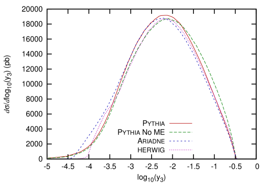
Figure 1: The $y_{3}$ spectra at parton level for P

YTHIA

, P

YTHIA

with matrix element reweighting switched off, A

RIADNE

and

HERWIG

.

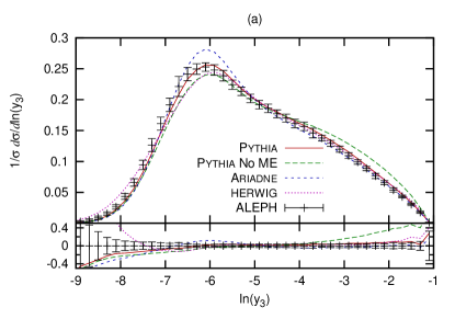
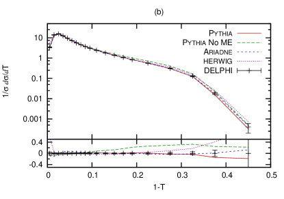
Figure 2: The $y_{3}$ spectra for charged and neutral particles (a) and the charged particle thrust spectra (b) for P

YTHIA

, P

YTHIA

with matrix element reweighting switched off, A

RIADNE

and

HERWIG

compared to ALEPH and DELPHI data. The in-sets at the bottom of the plots show the relative differences between the Monte Carlo results and data, $(\sigma_{\mathrm{MC}}-\sigma_{\mathrm{Data}})/\sigma_{\mathrm{Data}}$.

In figures 1 and 2 we present these distributions for the four generators A RIADNE (v 4.12)[13], HERWIG (v 6.510) [7] and P YTHIA (v 6.413) [37], which all are equipped with simple matrix element reweighting. We see that they all agree fairly well, which should come as no surprise since they have all been tuned to fit LEP data.

In figures 1 and 2 we also show the results from P YTHIA , with the matrix element reweighting switched off to give a sense of how large an effects we should expect from the matrix element corrections. We see that the main effect is that these distributions are clearly harder than the ones with matrix element reweighting.

We had planed to also include S HERPA [6] in this comparison and use it for the CKKW results. Unfortunately we discovered inconsistencies in the results and therefore decided not to use S HERPA at all in this study.

3.1 CKKW-L

We start by looking at the results from the CKKW-L scheme. Two implementations have been considered. We have used the original implementation[2] in A RIADNE and we have also made an implementation of the first order corrections using the transverse momentum ordered shower in P YTHIA [37, 41].

In A RIADNE the parton evolution is modeled by a dipole cascade [42, 20]. Unlike most other parton showers, the dipole cascade is based around $2\rightarrow 3$ partonic splittings rather than $1\rightarrow 2$. This model automatically includes the coherence effects from emitting gluons from colour-neighboring partons, which means that explicit angular ordering is not necessary. It also means that the first order matrix element $e^{+}e^{-}\rightarrow qg\bar{q}$ is already present in the cascade by construction. The ordering variable used in the cascade is a Lorentz-invariant transverse momentum measure

$$p_{\perp}^{2}=\frac{s_{12}s_{23}}{s_{123}},$$ (23)

where $s_{ij}$ are the invariant masses of the partons and index 2 indicates the emitted parton. This measure is then also used in the construction of the shower history in a procedure similar to the D ICLUS jet clustering algorithm[43], but including only physically allowed clusterings.

We have also implemented the CKKW-L scheme using the transverse-momentum ordered shower[41] in P YTHIA . This cascade exhibits the main features required by the CKKW-L scheme, namely that it is ordered in transverse momentum and that is has well-defined on-shell intermediate states. The ordering variable (also called $p_{\perp}$) is defined in the following way:

$$p_{\perp}^{2}=z(1-z)Q^{2}$$ (24)

$Q^{2}$ is the invariant mass of the produced parton and radiating parton and $z$ is the energy fraction of the radiating parton. The ordering of the shower is done in a way which incorporates coherence effects without requiring explicit angular ordering.

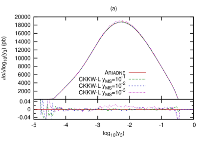
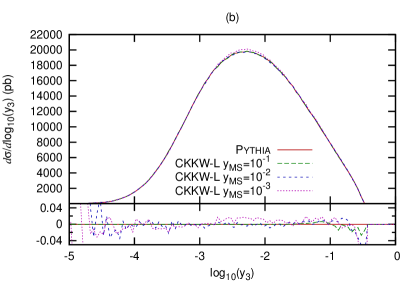
Figure 3: (a) The $y_{3}$ spectra at parton level for A

RIADNE

(the first order matrix element is included by construction) and for the A

RIADNE

implementation of CKKW-L corrections with different merging scales. (b) is the same for our P

YTHIA

implementation of CKKW-L corrections with different merging scales. The in-sets at the bottom of the plots show the relative differences between the CKKW-L results and the default shower, $(\sigma_{\mathrm{CKKW-L}}-\sigma_{\mathrm{Shower}})/\sigma_{\mathrm{Shower}}$.

There is one significant difference in the P YTHIA implementation, namely that the constructed history is no longer unique. In P YTHIA there are two possible ways for the gluon to be emitted (from the quark or the anti-quark), which means that there are two possible histories to be considered. One history is selected with a probability proportional to its branching probability.

In figure 3 we show the parton-level $y_{3}$ distribution for A RIADNE and transverse momentum ordered P YTHIA shower with matrix element reweighting. Both programs are compared to their respective CKKW-L implementations with different merging scales, and the figure shows that the cancellation is almost complete. There are some small discrepancy for the lowest cutoff of the order of 2%. This is because M AD E VENT generated the matrix element with massless u, d, s and c quarks, where as in A RIADNE and P YTHIA they are given a small mass, which causes a slight deviation in the emission probability. This discrepancy can be removed by setting the masses in A RIADNE and P YTHIA equal to the masses in M AD E VENT . No deviations, however, are visible below the merging scale.

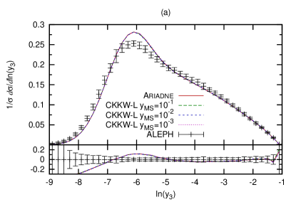
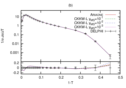
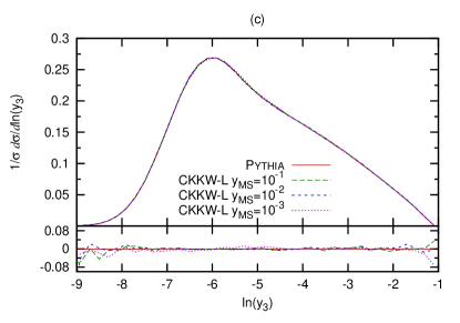
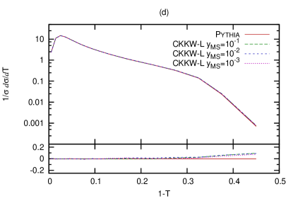
Figure 4: Charged plus neutral particle $y_{3}$ and charged particle thrust for the A

RIADNE

and P

YTHIA

implementation of CKKW-L corrections with different merging scales. Figure (a) includes a comparison to ALEPH data and (b) a comparison to DELPHI data, where figure (c) and (d) only compare to the default P

YTHIA

, since the $p_{\perp}$-ordered shower has not yet been tuned to data.

For completeness we show in figure 4 the comparison for the hadron-level observables $y_{3}$ and thrust for A RIADNE and $p_{\perp}$-ordered P YTHIA respectively. As expected from the parton-level results, there is no serious dependence on the merging scale.

3.2 CKKW

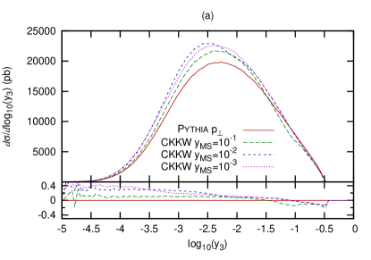
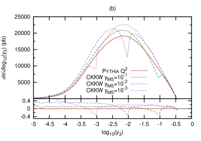
Figure 5: The $y_{3}$ spectra at parton level for P

YTHIA

with $p_{\perp}$-ordered (a) and virtuality ordered (b) shower (and with the first order matrix element reweighting included) and for our corresponding P

YTHIA

implementations of CKKW corrections with different merging scales.

The CKKW algorithm has been implemented using P YTHIA , with both the $p_{\perp}$-ordered and the virtuality ordered shower. The implementations are done according to the scheme described in section 2.2. The only difference is that none of the implementations use the Durham $k_{\perp}$ as ordering variables, therefore setting the starting scale is done differently. The scale of the quark and anti-quark is set to $E_{\mathrm{CM}}$ and the scale of the gluon is set to the $p_{\perp}$ of the reconstructed splitting for the $p_{\perp}$-ordered shower and the virtuality and angle of the splitting for the virtuality ordered shower. For the latter, the scheme is essentially equivalent to what is implemented in S HERPA . The results are shown in figure 5.

The results from the $p_{\perp}$ ordered shower show a smooth transition between the regions above and below the cutoff. This is to be expected since Durham $k_{\perp}$ is approximately equal to the $p_{\perp}$ in the shower, which means that the entire procedure becomes similar to CKKW-L with the exception that the Sudakov form factors are calculated according to an analytical approximation. The CKKW results show a slightly higher cross section than standard P YTHIA , which is attributed to the fact that in the analytical Sudakov form factors the approximate splitting functions are integrated over parts of phase space where they are negative. This means that Sudakov form factors cannot be interpreted as no-emission probabilities in the same way as in the shower and the end result is a slightly smaller suppression.

Figure 5b shows the results from the virtuality ordered shower and there are clear problems. Each CKKW curve has a dip right at the merging scale and for higher values of $y_{3}$ they are significantly above the default results from P YTHIA . One source of problems is that the shower can generate unordered emissions, since an emission which has a high vitruality can have a low $k_{\perp}$. This also changes which Sudakov form factor is applied to each region of phase space. A derivation of the problems that this can lead to for the lowest order process is presented in appendix A.

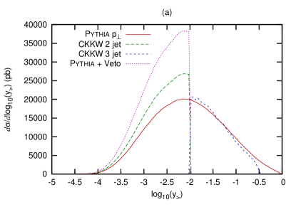
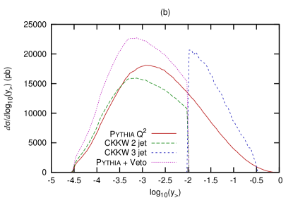
Figure 6: The maximum Durham $k_{\perp}$-value of any emission in the cascade for P

YTHIA

with $p_{\perp}$-ordered shower (and with the first order matrix element reweighting included) and for the two- and three-jet components in our P

YTHIA

implementation of CKKW corrections with a merging scale $y_{\mathrm{MS}}=10^{-2}$. An extra curve is included to show the two-jet contribution without the suppression from the analytic Sudakov form factor.

To further scrutinize the causes of the problems in the virtuality ordered CKKW implementation, we have studied the variable used for the shower veto which is the $k_{\perp}$-value of the individual emission. Figure 6 shows the maximum Durham $k_{\perp}$-value for the emissions in the shower. The results have been split into two and three-jet components of the CKKW implementation using P YTHIA $p_{\perp}$ and virtuality ordered shower.

The two-jet events in CKKW is produced by invoking the shower vetoing emissions above the merging scale and reweighting with an analytical Sudakov form factor. These two steps can be considered separately, which is illustrated in figure 6 by having a curve that only includes the veto and not the reweighting.

For the shower ordered in transverse momentum the three-jet contribution match the curve from running default P YTHIA fairly well above the merging scale. This is expected since the ordering in the transverse momentum ordered shower is fairly close to using Durham $k_{\perp}$-ordering. The two-jet contribution is similar in shape but is higher in cross section, which can be attributed to a smaller suppression from the analytical Sudakov form factors as compared to the form factors used in the shower. There is a discontinuity at the merging scale, but it is smoothed out by the shower causing the figure 5a to appear somewhat smooth.

With the virtuality ordered shower the results are quite different, which is caused by using two rather different scales. The problem is that emissions modifies the phase space for subsequent emissions, and by emitting the partons with highest virtuality first, the hardest emissions in $k_{\perp}$ are no longer allowed. When studying the hardest emission according to Durham $k_{\perp}$, this results in a shift to smaller values. This is why the P YTHIA curve is significantly below the three-jet CKKW curve in figure 6b. The sum of the two and three-jet contributions in figure 6b has two peaks with a clear dip in between. When the rest of the emissions are included this structure is somewhat smothed out, but the two peaks with a dip in between are clearly visible in figure 5b.

It is clear that one has to be a bit careful regarding the choice of shower and scales in CKKW. One CKKW implementation based on HERWIG was published in [3] and the results were consistent only after a significant amount of tuning of scale parameters. A similar procedure could probably be used to make our results more consistent, but it would add extra somewhat arbitrary parameters to the model. The problem with the ordering of the emissions also leads to a different colour structure in the events, which was pointed out in [26].

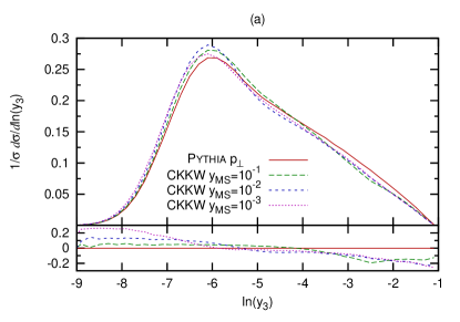
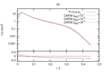
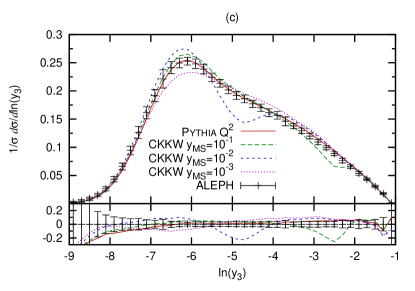
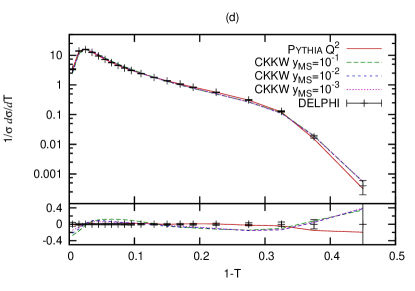
Figure 7: Charged plus neutral particle $y_{3}$ and charged particles thrust for our P

YTHIA

implementation of CKKW corrections with transverse momentum and virtuality ordered showers and using different merging scales. Figure (c) includes a comparison to ALEPH data and (d) a comparison to DELPHI data, where figure (a) and (b) only compare to the default P

YTHIA

, since the transverse momentum ordered shower has not yet been tuned to data.

Finally we show the consequences for two experimental observables in figure 7. Again, the results of the $p_{\perp}$-ordered shower has only been compared to the default P YTHIA , since it is not yet tuned to data. The $p_{\perp}$-ordered plots show significant lower values at high $y_{3}$ and low thrust, which is the result of the excess in cross section for two-jet events. We also see some trace of the discontinuities in figure 6a, but they have been smoothed out by the shower and hadronization. The results from the virtuality ordred shower shows the same dips in the $y_{3}$ distribtion as in the parton-level plots. The dips are not visible in the thrust plot, but there are significant deviations from default P YTHIA .

3.3 Pseudo-Shower

We have implemented the Pseudo-Shower[3] algorithm using matrix element events generated with M AD E VENT and using P YTHIA with both virtuality ordered and $p_{\perp}$-ordered parton shower. The implementation has been done with the following definition for the jet clustering.

$$d_{ij}\equiv m_{ij}^{2}E_{i}E_{j}/(E_{i}+E_{j})^{2}$$ (25)

This is equivalent to the measure in the L UCLUS algorithm (and to the $k_{\perp}$-definition in eq. (24)) in the limit of massless particles. The jet algorithm was used both to define the merging scale and the clustering of jet observables as specified by the merging scheme. $\alpha_{\mathrm{s}}$-reweighting has been introduced using the scales from the jet clustering, which is happens to be the same scale definition that is used in the $\alpha_{\mathrm{s}}$ evaluation in the P YTHIA shower.

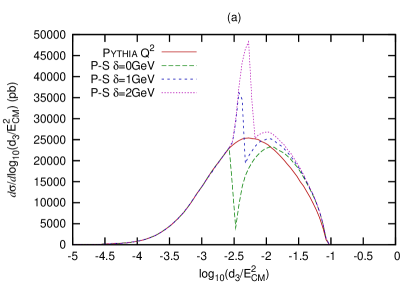
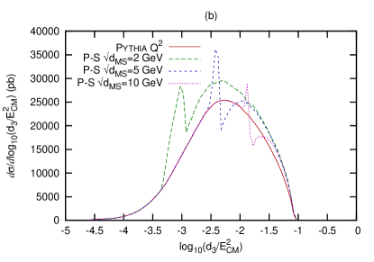
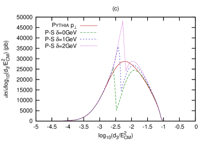
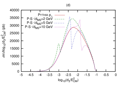
Figure 8: The $d_{3}$ spectra at parton level for P

YTHIA

(with first order matrix element reweighting included) and for our implementation of the Pseudo-Shower algorithm using both the vituality ordered and the $p_{\perp}$-ordered shower. (a) and (c) show the effects of different valuses of the fudge factor $\delta$ with a merging scale of $\sqrt{d_{\mathrm{MS}}}=5$ GeV. (b) and (d) show the results from different values of the merging scale $d_{\mathrm{MS}}$ using a fudge factor $\delta=1$ GeV.

The first thing that is investigated is the effects of different values of the fudge factor $\delta$ introduced in section 2.4. The most sensitive distribution for checking the effects is the same variable as the merging scale. Figure 8a and 8c show the $d_{3}$ distribution at parton level for three different values of $\delta$. In both figures the curve that shows the smallest deviations is $\delta=1$ GeV, and this value is used in the rest of this section. It is clear that there is no smooth transition between the matrix element and parton shower phase space.

Figure 8 also showes what happens if the merging scale is varied. The discontinuities persist for all three values of the merging scale and for the two different showers and the results are heavily dependent on the merging scale. The problem is a conseqence of using different ways of defining the scales in the algorithm, which we discussed in section 2.4. The results in the rest of this section focuses on the Pseudo-Shower implemenation with a vituality ordered shower, since this was used in the original publication [3].

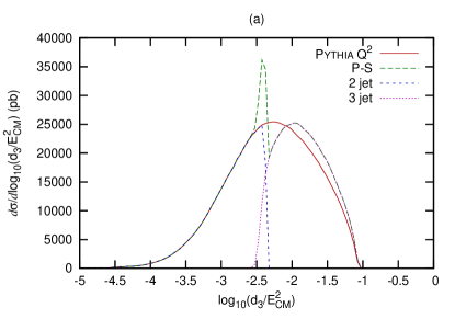
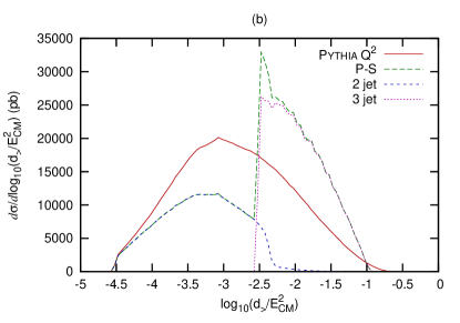
Figure 9: The Pseudo-Shower results, with $\sqrt{d_{\mathrm{MS}}}=5$ GeV and $\delta=1$ GeV, split into two- and three-jet components compared to the default shower in P

YTHIA

(with first order matrix element reweighting included). (a) shows the $d_{3}$ distribution at parton level and (b) is the largest $d$-value of the emissions in the shower.

To demonstrate the different scales used in the algorihtm, the Pseudo-Shower results have been split up into the contributions from the two- and three-jet matrix elements. Figure 9a shows the $d_{3}$ distribution, where it is clear that the two-jet contribution displays a sharp cut, but not the three-jet component. On the other hand, when the largest $d$-value of the emissions in the shower is plotted in figure 9b, the three-jet component has a sharp cut but not the two-jet curve. This illustrates that different scales are used for the different jet multiplicities and this is the reason for the problems that appear close to the merging scale.

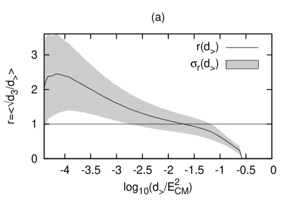
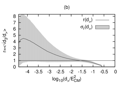
Figure 10: The average ratio between the clustering scale $d_{3}$ for partonic jets and the generated maximum splitting scale $\rho_{3}$ in the cascade as a function of the latter. The shaded area indicates the standard deviation of the ratio. Both scales are defined as in eq. (25). (a) is for the $p_{\perp}$-ordered shower in P

YTHIA

, while (b) is for the virtuality ordered one.

To further illustrate the complication with mixing scales for parton splittings and partonic jets, we show in figure 10 the variation of the ratio between the $d_{3}$ scale on partonic jet level and the largest generated scale in the parton shower $d_{>}$. In a strongly ordered shower this ratio should ideally be unity, especially for the $p_{\perp}$-ordered P YTHIA shower in figure 10a. However, we find that this is far from the case. Especially for the virtuality ordered shower in figure 10b, the correlation between the different scales is very weak.

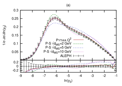
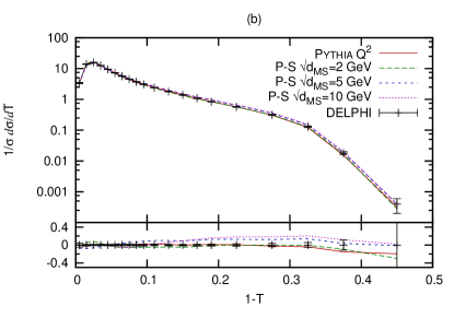
Figure 11: The charged plus neutral particle $y_{3}$ spectra (a) and charged particle thrust spectra (b) for P

YTHIA

(with first order matrix element reweighting included) and for our implementation of the Pseudo-Shower algorithms with different merging scales and $\delta=1$ GeV compared to ALEPH and DELPHI data.

Finally two experimental observables are plotted, namely the normalized $y_{3}$ distribution for charged and neutral particles and the charged particles thrust, which are shown in figure 11. Hadronization smoothes out most of the discontinuities shown in earlier figures, but it is clear that there are still problems. The plots show deviations from data and the results are not be independent of the merging scale.

3.4 MLM

To test MLM for $e^{+}e^{-}$ a merging scheme and a parton–jet distance need to be chosen. Most of the MLM implementations use cone algorithms to achieve this purpose. In the case of $e^{+}e^{-}$, we think that a $k_{\perp}$-based clustering algorithm is a better choice. We have therefore decided to use the Durham $k_{\perp}$ algorithm to define the merging scale and matrix element cutoff.

When it comes to selecting a measure for the parton–jet distance, the natural choice would be the $k_{\perp}$-distance between the jet and the parton. The problem with this approach is that since the $k_{\perp}$-measure includes the minimum of the two energies it means that soft partons can match jets at very wide angles, which leads to problems with convergence. Instead we modified the distance to only use the jet energy.

$$y_{\mathrm{jet,parton}}=2E_{jet}^{2}(1-\cos(\theta_{\mathrm{jet,parton}}))/E_{CM}^{2}$$ (26)

For the highest multiplicity treatment we follow the M AD E VENT implementation in [11]. For each highest multiplicity event, jets are reconstructed at a scale which is the maximum of the merging scale and the smallest distance between the partons in the matrix element level event, $\max(y_{\mathrm{MS}},y_{N})$. This scale is also used when matching the jets to partons. This allows extra jets to be produced if they are softer than those from the matrix element.

The algorithm has been implemented using M AD E VENT to generate the matrix element event and both HERWIG and P YTHIA has been used to shower the events. Before we move on to the results of the merging, some important aspects of the showers need to be explained.

Step 3 in the algorithm (described in section 2.5), where the shower is invoked, depends on how the state received from the matrix element is treated in the parton shower program. For the analysis of the merging it is important to understand how the events are treated internally. In particular the states containing soft and collinear partons require extra scrutiny since the matrix element cross section is divergent in these regions.

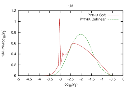
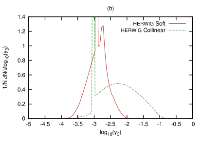
Figure 12: The $y_{3}$ spectra at parton level for P

YTHIA

(a) and

HERWIG

(b) when starting from a state with a soft or a collinear gluon with a merging scale of $y=10^{-3}$ and the scale in the Les Houches interface set to $E_{\mathrm{CM}}$.

In the P YTHIA implementation of the Les Houches interface, the limiting factors for the radiation are the scale from the Les Houches interface, which is used as a veto, and the energy of the partons, which become the maximum kinematically allowed value for the invariant mass. No extra vetoes are applied for emissions at a wide angles. This means that even when soft or collinear partons are present some events have a lot of emissions, assuming that the scale in the Les Houches interface is set to a high value. Figure 12a shows the $y_{3}$ spectra for a state with a soft gluon and for one with a collinear gluon with $y_{3}=10^{-3}$ and the scale set to $E_{\mathrm{CM}}$. It is obvious from the figure that a soft or collinear parton does not limit the emissions significantly.

HERWIG

uses a different strategy for the internal choices of scale. Each parton is given a starting scale which is equal to the product of the four-momentum of itself and its color neighbour (if a parton has two color neighbours one is chosen at random). The parton is then boosted to the frame where it is at a right angle compared to its color neighbour and the shower invoked. Any scale set in the Les Houches interface is included as a veto on the transverse momentum (approximately given by eq. (25)) of the emissions. The $y_{3}$ histogram from a HERWIG shower are shown in figure 12b starting from the same states and from the same scale as in figure 12a. From the figure one can tell that a soft parton limits the emission from the shower quite drastically, but for a collinear parton about half of the events show significant jet activity.

Clearly, the way soft and collinear events from the matrix element give rise to hard emissions influences the jet matching veto, which is assumed to give the Sudakov suppression of these events, and the different choices of scales in the shower can have a big impact on these Sudakov form factors. This means that one has to be very careful with generalizing the MLM algorithm to different showers.

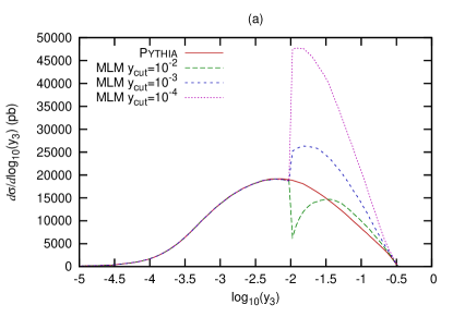
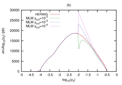
Figure 13: (a) The $y_{3}$ spectra at parton level for default P

YTHIA

and our P

YTHIA

implementation of the MLM algorithm for $y_{\mathrm{MS}}=10^{-2}$ and for different values of the matrix element cutoff. (b) shows the same for

HERWIG

.

The first thing that needs to be verified with our MLM implementation is if the results converge when the matrix element cutoff is lowered. The results of the merging are shown in figure 13 for P YTHIA and HERWIG , with a merging scale of $y_{3}=10^{-2}$ and three different values for the cutoff. No sign of convergence is visible in the figure.

The problem is related to how HERWIG and P YTHIA treats input with soft or collinear partons. The MLM algorithm assumes that soft and collinear partons cannot produce independent jets when fed into the shower. From the earlier figures it is clear that P YTHIA can produce extra jets both for soft and collinear partons, whereas HERWIG can only produce extra jets for collinear partons. This is the reason why P YTHIA diverges faster.

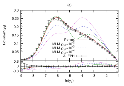
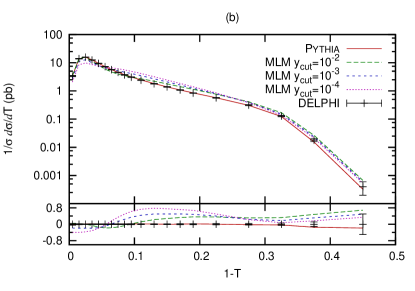
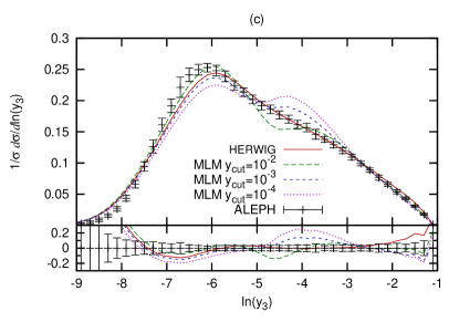
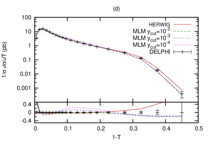
Figure 14: The charged plus neutral particle $y_{3}$ spectra (a) and the charged particle thrust spectra (b) for default P

YTHIA

and our P

YTHIA

implementation of the MLM algorithm for three different values of the matrix element cutoff. The

HERWIG

results are shown in (c) and (d) respectively.

The changes to the parton-level spectra is also visible in the hadron-level observables, shown in figure 14. It is clear that changing the matrix element cutoff also affects the event shape, which diminishes the predictive power of the model.

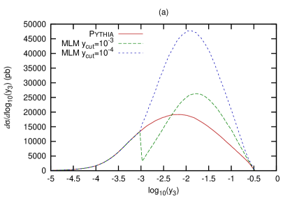
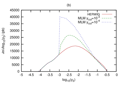
Figure 15: (a) The $y_{3}$ spectra at parton level for default P

YTHIA

and our P

YTHIA

implementation of the MLM algorithm for $y_{\mathrm{MS}}=10^{-3}$ and for two different values of the matrix element cutoff. (b) shows the same for

HERWIG

.

In figure 15 the parton-level $y_{3}$-spectra is shown with a lower merging scale. Generally one can say that the discrepancies as compared to the standard P YTHIA and HERWIG become even bigger. In HERWIG , configurations with soft gluons cannot generate hard emissions, which means a large fraction of these events are kept. There is a pole in the soft gluon limit and the cross sections for these events are therefore rather large, which leads to a continued rise of the cross section of the MLM-corrected curve for low values of $y_{3}$, clearly visible in figure 15b.

The examples above show that the MLM algorithm is very sensitive to how emission are generated and it appears to be quite tough to fix this problem. If the shower generates an emission it risks influencing things at higher jet scale and if emissions are suppressed it is not possible to control the rise of the cross section near the soft and collinear limits. In fact, even if the problems described in this section can somehow be resolved, the more fundamental problem, described in section 2.5, that MLM uses the wrong type of Sudakov form factors remains unsolved.

4 Conclusions

In the previous sections, we have studied in some detail the behavior of four suggested algorithms, or schemes, for merging fixed order, tree-level matrix element generators with parton shower generators. We have done so by considering the simplest possible case of the leading order correction to the $\mathrm{e}^{+}\mathrm{e}^{-}\to$ hadrons process. This may not be an important use case for these merging schemes, but since it is such a simple process it is fairly easy to check whether the schemes actually accomplishes what they set out to do, namely to correctly populate the phase space above the merging scale with partons described by the full matrix element, and with emission from the parton shower below, and that they do so while correctly resumming large logarithmic contributions from soft and collinear divergencies. In addition, for this process we also have the “correct” answer available, obtained by a simple reweighting of the hardest emission in the parton shower.

Our main finding is that of the four schemes considered, only CKKW and CKKW-L meets the requirements and that even CKKW has some problems when using a parton shower with an ordering variable which is very different from the clustering variable used for the merging scale.

For CKKW-L it was claimed in [2] that the cancellation of the dependence on the merging scale is complete when using the A RIADNE dipole shower. Here we show this explicitly and also show that it is still true when using the transverse momentum ordered shower in P YTHIA . This is not a completely trivial result, because it involves an additional ambiguity in how to reconstruct the shower history for P YTHIA which is not present in A RIADNE .

In the CKKW case we also find a near complete cancellation of the merging scale dependence when using the $p_{\perp}$-ordered P YTHIA shower. However, when using the virtuality ordered shower in P YTHIA , we find a clear mismatch near the merging scale, and we trace this mismatch to different treatments of the no-emission probability from the gluon when it is emitted above and below the merging scale, and from possible problems in the parton shower when unordered emissions are allowed. These problems occur when the ordering variable is very different from the Durham $k_{\perp}$-measure used for the merging scale, which is true for the virtuality ordering, but not for the $p_{\perp}$-ordered shower. We expect that this is also the origin of the mismatches found in the CKKW implementation in HERWIG [3], where an elaborate tuning of the scales used in the Sudakov and $\alpha_{\mathrm{s}}$-reweighting was needed to minimize the merging scale dependence. Most likely a similar retuning can be done in the case of the virtuality ordered shower in P YTHIA .

For Mrennas Pseudo-Shower scheme, we find that the problems are much more severe. The main problem is that cuts made on parton level for the matrix element are made on the partonic jet level for the parton shower, and we show that this can never give the clean separation of phase spaces needed to have independence on the merging scale. This leads to a severe underestimate of the three-jet rate just above the merging scale. The fudge factor introduced in [3] can be tuned to hide the problem, but at the expense of overestimating the three-jet rate below the merging scale due to double-counting.

The MLM scheme is the simplest one to implement, in that it allows the use of any parton shower generator without modifying its internal behavior. It also uses partonic jet level cuts, but contrary to the Pseudo-Shower it tries to avoid mixing them with cuts on the few parton level. Nevertheless, an extra parton-level generation cut is needed for the matrix element. Supposedly the results should be independent on this generation cut as long as it is sufficiently smaller than the merging scale. However, we have found that this is not the case, and that the result is very sensitive to how the kinematics of the initial parton state limits emissions from the chosen parton shower. If the emissions are not limited, events generated close to the generation cut will always have a finite possibility to end up above the merging scale, which makes the scheme very sensitive to the generation cut. If, on the other hand, the emissions are limited by the kinematics, there is no possibility to obtain the necessary Sudakov suppression of soft and collinear divergencies. It is not inconceivable that the generation cut can be tuned, possibly together with the scale used in the $\alpha_{\mathrm{s}}$-weighting, to get reasonably smooth distributions, but we feel that this is just hiding the fact that the MLM scheme has serious flaws.

Having done this investigation of the behavior of the algorithms for the simplest possible process, the question is if we can make some conclusions for more complicated processes. Or course, if a scheme does not handle this simple process well, it is not likely that the situation will improve for more complicated ones. But also in the case of CKKW-L, complications may occur.

As we go to higher parton multiplicities in the matrix element, we expect that the actual matrix element correction becomes larger, necessarily giving rise to discontinuities near the merging scale. These discontinuities should disappear as the merging scale is lowered and the parton shower splittings become a good approximation to the full matrix element. However, for this to work there must not be any artificial dependencies on the merging scale in the merging algorithm as such, which we have seen is not the case for all schemes.

The really interesting processes are in hadron collisions, where e.g. the standard model production of a $W$ together with several hard jets is an important background to almost any search for new phenomena. Here the matching is complicated as the parton showers also includes initial state evolution of the incoming partons. Also, care must be taken to treat the parton densities in a consistent way. This was first investigated for the CKKW scheme in [5], and later for A RIADNE implementation of CKKW-L in [12]. For the latter it was shown that the merging scale dependence does indeed cancel for the leading order correction to $W$-production. Although it has not been checked explicitly for the other schemes, there is no reason to expect that the problems we have found in this paper will go away.

Having said all this, we must ask ourselves how severe the deficiencies we have found here would be for practical applications at e.g. the LHC. We are, after all, dealing with tree-level matrix elements and leading log parton showers which means we will in any case expect large scale dependencies. And surely these deficiencies results in much smaller uncertainties as compared to using parton showers without matrix element corrections. Indeed, it was shown in [11] that CKKW, CKKW-L and different MLM implementations all give consistent results for realistic experimental observables within reasonable variations of the scales used in $\alpha_{\mathrm{s}}$ and parton densities. In fact the most severe disagreement found was for the A RIADNE implementation of CKKW-L. However, this had nothing to do with the merging scheme, but is a consequence of the radically different treatment of the phase space available for initial-state radiation in A RIADNE as such, which includes a resummation of some logarithms of $x$, not present in conventional initial-state showers.

In [1] a large effort was put into showing that the dependence of the merging scale vanishes at next-to-leading logarithmic accuracy for CKKW, at least for a shower which is ordered in the Durham $k_{\perp}$ variable. Here we have shown that for the three-jet observables considered here, the dependence vanishes completely for CKKW-L. For the Pseudo-shower, the situation is more difficult to analyze. In the strongly ordered limit we argue that it is equivalent to CKKW-L, which indicates that the dependence on the merging scale should cancel, at least to leading double-logarithmic accuracy, nevertheless the dependence is quite large in absolute numbers. For MLM, it is clear that for the observables considered here, it is questionable if it can reproduce the correct Sudakov form factors, indicating a dependence on the merging scale (or rather the cutoff in the matrix element generation) already on the leading double-logarithmic level. We plan to return in a future publication with a more formal investigation of the logarithmic accuracy of the merging scales.

In absolute numbers, we have seen that the Pseudo-Shower and the MLM schemes, and even CKKW for some parton showers, have problems with correctly populating different regions of phase space. And even if this can be smoothed out by introducing additional cuts on the matrix element generation (for MLM), a fudge factor (for Pseudo-Shower) or separately varying the scale in the $\alpha_{\mathrm{s}}$ and Sudakov reweighting (for CKKW with HERWIG [3]) it necessarily means introducing extra parameters which need to be tuned. Indeed, it is not inconceivable that these extra parameters need to be tuned differently for different processes and merging scales, and maybe even for different observables. As a consequence, the predictability of the models will be reduced.

Appendix A Different scale definitions in CKKW

To illustrate the origin of the discontinuities found for CKKW when used with the virtuality-ordered shower in P YTHIA , we here look at the somewhat artificial example of calculating the differential exclusive three-jet rate, where we use the notation introduced in section 2.3.

Assume the parton shower has ordering in $\rho$, and has auxiliary splitting variables, $\vec{x}$, and that the Durham $k_{\perp}$-measure can be written as a function of these variables, $y=y(\rho,\vec{x})$. Now we can write the differential exclusive three-jet rate above some $\rho_{0}$ for the plain parton shower case:

$$\frac{d\sigma_{3}^{\mathrm{PS}}}{\sigma_{0}}=\Delta_{S_{2}}^{\mathrm{PS}}(\rho_{\max},\rho)\Gamma_{S_{2}}^{\mathrm{PS}}(\rho,\vec{x})\Delta_{S_{3}}^{\mathrm{PS}}(\rho,\rho_{0})d\rho\,d^{k}\vec{x}$$ (27)

where $\Delta_{S_{2}}(\rho_{\max},\rho)$ is the Sudakov corresponding to the no-emission probability from the two-parton state above $\rho$, and $\Delta_{S_{3}}(\rho,\rho_{0})$ is the no-emission probability from the three-parton state below $\rho$. We can also write the corresponding rate for the CKKW scheme:

$$\frac{d\sigma_{3}^{\mathrm{CKKW}}}{\sigma_{0}} \approx \Delta_{S_{2}}^{\mathrm{CKKW}}(y_{\max},y)\Gamma_{S_{2}}^{\mathrm{ME}}(\rho,\vec{x})\times$$ (28)

$$\Delta_{S_{2}}^{\mathrm{PS}}(\rho_{\max},\rho;<y)\Delta_{S_{3}}^{\mathrm{PS}}(\rho,\rho_{0};<y)d\rho\,d^{k}\vec{x}$$

where $\Delta_{S_{2}}^{\mathrm{CKKW}}(y_{\max},y)$ is the analytic Sudakov form factor used for reweighting, and $\Delta_{S_{3}}^{\mathrm{PS}}(\rho,\rho_{0};<y)$ is the parton shower no-emission probability from the three-parton state between $\rho$ and $\rho_{0}$ excluding phase space region corresponding to the vetoed emissions with Durham $k_{\perp}$ above $y(\rho,\vec{x})$. $\Delta_{S_{2}}^{\mathrm{PS}}(\rho_{\max},\rho;<y)$ is the corresponding no-emission probability for the two-parton state, which approximates the no-emission probability for the three-parton state above the scale $\rho$ where the gluon is not allowed to radiate — an approximation which is valid as long as the gluon is not too hard. Now the CKKW Sudakov can be approximately written as the no-emission probability

$$\Delta_{S_{2}}^{\mathrm{CKKW}}(y_{\max},y) \approx \Delta_{S_{2}}^{\mathrm{PS}}(\rho_{\max},\rho_{0};>y)=\Delta_{S_{2}}^{\mathrm{PS}}(\rho_{\max},\rho;>y)\Delta_{S_{2}}^{\mathrm{PS}}(\rho,\rho_{0};>y),$$ (29)

where the $>y$ notation indicates that only emissions with Durham $k_{\perp}$ above $y$ are considered. Also, we can write

$$\Delta_{S_{2}}^{\mathrm{PS}}(\rho_{\max},\rho)=\Delta_{S_{2}}^{\mathrm{PS}}(\rho_{\max},\rho;>y)\Delta_{S_{2}}^{\mathrm{PS}}(\rho_{\max},\rho;<y)$$ (30)

and

$$\Delta_{S_{3}}^{\mathrm{PS}}(\rho,\rho_{0})=\Delta_{S_{3}}^{\mathrm{PS}}(\rho,\rho_{0};>y)\Delta_{S_{3}}^{\mathrm{PS}}(\rho,\rho_{0};<y)$$ (31)

We can now rewrite the two three-jet rates as

$$\frac{d\sigma_{3}^{\mathrm{PS}}}{\sigma_{0}} = \Gamma_{S_{2}}^{\mathrm{PS}}(\rho,\vec{x})\Delta_{S_{2}}^{\mathrm{PS}}(\rho_{\max},\rho;>y)\Delta_{S_{2}}^{\mathrm{PS}}(\rho_{\max},\rho;<y)\times$$

$$\Delta_{S_{3}}^{\mathrm{PS}}(\rho,\rho_{0};>y)\Delta_{S_{3}}^{\mathrm{PS}}(\rho,\rho_{0};<y)d\rho\,d^{k}\vec{x}$$

$$\frac{d\sigma_{3}^{\mathrm{CKKW}}}{\sigma_{0}} = \Gamma_{S_{2}}^{\mathrm{ME}}(\rho,\vec{x})\Delta_{S_{2}}^{\mathrm{PS}}(\rho_{\max},\rho;>y)\Delta_{S_{2}}^{\mathrm{PS}}(\rho,\rho_{0};>y)\times$$ (32)

$$\Delta_{S_{2}}^{\mathrm{PS}}(\rho_{\max},\rho;<y)\Delta_{S_{3}}^{\mathrm{PS}}(\rho,\rho_{0};<y)d\rho\,d^{k}\vec{x}$$

And we find that the only difference, besides the desired $\Gamma_{S_{2}}^{\mathrm{PS}}\to\Gamma_{S_{2}}^{\mathrm{ME}}$, is that in the plain shower has a no-emission probability $\Delta_{S_{3}}^{\mathrm{PS}}(\rho,\rho_{0};>y)$ where CKKW has $\Delta_{S_{2}}^{\mathrm{PS}}(\rho,\rho_{0};>y)$. This can be seen as an extra suppression in the plain parton shower due to the no-emission probability from the gluon at a shower scale below $\rho$ but at a Durham $k_{\perp}$-scale above $y$. Now if the ordering variable $\rho$ is close to the Durham $k_{\perp}$, this region will be very small and the mismatch will be small, as we saw in the case of the $p_{\perp}$-ordered P YTHIA shower. But for the virtuality ordering in P YTHIA we have

$$y=\min\left(\frac{z}{1-z},\frac{1-z}{z}\right)\frac{Q^{2}}{E_{\mathrm{CM}}^{2}}$$ (33)

and similarly for the angular ordering variable, $\xi$, in HERWIG we have

$$y=\min(z^{2},(1-z)^{2})\frac{E^{2}\xi}{E_{\mathrm{CM}}^{2}},$$ (34)

(where $E$ is the energy of the parent parton in the splitting) and, hence, the region can become quite large, especially in the regions $z\to 0$ or $1$, where the probability of an emission is large. We note, however, that in P YTHIA the effect is limited by the presence of an additional angular ordering veto in addition to the virtuality ordering.

References

- [1] S. Catani, F. Krauss, R. Kuhn, and B. R. Webber JHEP 11 (2001) 063, hep-ph/0109231.
- [2] L. Lönnblad JHEP 05 (2002) 046, hep-ph/0112284.
- [3] S. Mrenna and P. Richardson JHEP 05 (2004) 040, hep-ph/0312274.
- [4] M. Mangano, “The so-called MLM prescription for ME/PS matching.” http://www-cpd.fnal.gov/personal/mrenna/tuning/nov2002/mlm.pdf. Talk presented at the Fermilab ME/MC Tuning Workshop, October 4, 2002.
- [5] F. Krauss JHEP 08 (2002) 015, hep-ph/0205283.
- [6] T. Gleisberg et al. JHEP 02 (2004) 056, hep-ph/0311263.
- [7] G. Corcella et al. JHEP 01 (2001) 010, hep-ph/0011363.
- [8] F. Krauss, A. Schalicke, S. Schumann, and G. Soff Phys. Rev. D70 (2004) 114009, hep-ph/0409106.
- [9] F. Krauss, A. Schalicke, S. Schumann, and G. Soff Phys. Rev. D72 (2005) 054017, hep-ph/0503280.
- [10] T. Gleisberg, F. Krauss, A. Schalicke, S. Schumann, and J.-C. Winter Phys. Rev. D72 (2005) 034028, hep-ph/0504032.
- [11] J. Alwall et al. Eur. Phys. J. C53 (2008) 473–500, arXiv:0706.2569 [hep-ph].
- [12] N. Lavesson and L. Lönnblad JHEP 07 (2005) 054, hep-ph/0503293.
- [13] L. Lönnblad Comput. Phys. Commun. 71 (1992) 15.
- [14] T. Sjöstrand, L. Lönnblad, S. Mrenna, and P. Skands hep-ph/0308153.
- [15] M. L. Mangano, M. Moretti, F. Piccinini, R. Pittau, and A. D. Polosa JHEP 07 (2003) 001, hep-ph/0206293.
- [16] J. Alwall et al. arXiv:0706.2334 [hep-ph].
- [17] A. Cafarella, C. G. Papadopoulos, and M. Worek arXiv:0710.2427 [hep-ph].
- [18] M. L. Mangano, M. Moretti, and R. Pittau Nucl. Phys. B632 (2002) 343–362, hep-ph/0108069.
- [19] M. L. Mangano, M. Moretti, F. Piccinini, and M. Treccani JHEP 01 (2007) 013, hep-ph/0611129.
- [20] G. Gustafson and U. Pettersson Nucl. Phys. B306 (1988) 746.
- [21] M. Bengtsson and T. Sjostrand Phys. Lett. B185 (1987) 435.
- [22] M. H. Seymour Nucl. Phys. B436 (1995) 443–460, hep-ph/9410244.
- [23] M. H. Seymour Comp. Phys. Commun. 90 (1995) 95–101, hep-ph/9410414.
- [24] S. Frixione and B. R. Webber JHEP 06 (2002) 029, hep-ph/0204244.
- [25] S. Frixione and B. R. Webber hep-ph/0612272.
- [26] P. Nason JHEP 11 (2004) 040, hep-ph/0409146.
- [27] P. Nason and G. Ridolfi JHEP 08 (2006) 077, hep-ph/0606275.
- [28] S. Frixione, P. Nason, and C. Oleari JHEP 11 (2007) 070, arXiv:0709.2092 [hep-ph].
- [29] M. Kramer, S. Mrenna, and D. E. Soper Phys. Rev. D73 (2006) 014022, hep-ph/0509127.
- [30] Z. Nagy and D. E. Soper JHEP 10 (2005) 024, hep-ph/0503053.
- [31] Z. Nagy and D. E. Soper JHEP 09 (2007) 114, arXiv:0706.0017 [hep-ph].
- [32] W. T. Giele, D. A. Kosower, and P. Z. Skands arXiv:0707.3652 [hep-ph].
- [33] C. W. Bauer, F. J. Tackmann, and J. Thaler arXiv:0801.4026 [hep-ph].
- [34] C. W. Bauer, F. J. Tackmann, and J. Thaler arXiv:0801.4028 [hep-ph].
- [35] S. Catani, Y. L. Dokshitzer, M. Olsson, G. Turnock, and B. R. Webber Phys. Lett. B269 (1991) 432–438.
- [36] A. Schaelicke and F. Krauss hep-ph/0503281.
- [37] T. Sjostrand, S. Mrenna, and P. Skands JHEP 05 (2006) 026, hep-ph/0603175.
- [38] E. Boos et al. hep-ph/0109068.
- [39] ALEPH Collaboration, A. Heister et al. Eur. Phys. J. C35 (2004) 457–486.
- [40] DELPHI Collaboration, P. Abreu et al. Z. Phys. C73 (1996) 11–60.
- [41] T. Sjostrand and P. Z. Skands Eur. Phys. J. C39 (2005) 129–154, hep-ph/0408302.
- [42] G. Gustafson Phys. Lett. B175 (1986) 453.
- [43] L. Lönnblad Z. Phys. C58 (1993) 471–478.
- [44] T. Sjostrand Comput. Phys. Commun. 28 (1983) 229.