General Features of Supersymmetric Signals at the ILC: Solving the LHC Inverse Problem

Abstract

We present the first detailed, large-scale study of the Minimal Supersymmetric Standard Model (MSSM) at a $\sqrt{s}=500$ GeV International Linear Collider, including full Standard Model backgrounds and detector simulation. We investigate 242 points in the MSSM parameter space, which we term models, that have been shown by Arkani-Hamed et al. to be difficult to study at the LHC. In fact, these points in MSSM parameter space correspond to 162 pairs of models which give indistinguishable signatures at the LHC, giving rise to the so-called LHC Inverse Problem. We first determine whether the production of the various SUSY particles is visible above the Standard Model background for each of these parameter space points, and then make a detailed comparison of their various signatures. Assuming an integrated luminosity of 500 fb^-1, we find that only 82 out of 242 models lead to visible signatures of some kind with a significance $\geq 5$ and that only 57(63) out of the 162 model pairs are distinguishable at $5(3)\sigma$. Our analysis includes PYTHIA and CompHEP SUSY signal generation, full matrix element SM backgrounds for all $2\to 2\,,2\to 4$, and $2\to 6$ processes, ISR and beamstrahlung generated via WHIZARD/GuineaPig, and employs the fast SiD detector simulation org.lcsim.

I Introduction

The LHC is scheduled to begin operations within a year and is expected to change the landscape of particle physics. While the Standard Model (SM) does an excellent job describing all strong interaction and electroweak data to date LEPEWWG ; Yao:2006px , there are many reasons to be dissatisfied with the SM. Chief among them are issues related to electroweak symmetry breaking. As is by now well-known, the SM with a single Higgs doublet that is responsible for generating the masses of both the electroweak gauge bosons and fermions encounters difficulties associated with stability, fine-tuning, and naturalness. Addressing these issues necessitates the existence of new physics at the Terascale. To this end, numerous creative candidate theories that go beyond the SM have been proposed and many yield characteristic signatures at the LHC. When the ATLAS and CMS detectors start taking data at the LHC, they will explore this new territory. They will then begin the process of identifying the nature of physics at the Terascale and of determining how it fits into a broader theoretical structure.

Of the several proposed extensions of the SM that resolve the issues mentioned above, the most celebrated is Supersymmetry (SUSY) SUSY . Our working hypothesis in this paper is that SUSY has been discovered at the LHC, i.e., that new particles have been observed and it has been determined that they arise from Supersymmetry. Identifying new physics as Supersymmetry is in itself a daunting task, and we would be lucky to be in such a situation! However, even in this optimistic scenario, much work would be left to be done as SUSY is a very broad framework. We would want to know which version of SUSY nature has realized and for this we would need to map the LHC observables to the fundamental parameters in the weak scale SUSY Lagrangian. A question that would arise is whether this Lagrangian can be uniquely reconstructed given the full set of LHC measurements. This issue has been recently quantified in some detail by the important work of Arkani-Hamed, Kane, Thaler and Wang (AKTW) Arkani-Hamed:2005px , which demonstrates what has come to be known as the LHC Inverse Problem. AKTW found that even in the simplest realization of Supersymmetry, the Minimal Supersymmetric Standard Model (MSSM), such a unique mapping does not take place given the LHC observables alone and that many points in the MSSM parameter space cannot be distinguished from each other. Here, we extend their study and examine whether data from the proposed International Linear Collider (ILC) can uniquely perform this inverse mapping and resolve the model degeneracies found by AKTW.

In brief, AKTW considered a restricted Lagrangian parameter subspace of the MSSM. They forced all SUSY partner masses to lie below 1 TeV (in order to obtain a large statistical sample at the LHC), fixed the third generation $A$-terms to 800 GeV and set the pseudoscalar Higgs mass to be 850 GeV. Points in the MSSM parameter space, hereafter referred to as models for brevity, were generated at random with the conditions that $\tan\beta$ lies in the range 2-50, squark and gluino Lagrangian mass terms lie above 600 GeV, and Lagrangian mass terms for the non-strongly interacting particles be greater than 100 GeV. 43,026 models were generated in this 15-dimensional parameter space under the assumption that all parameter ranges were uniformly distributed, i.e., flat priors were employed. No further constraints, such as the LEP lower bound on the Higgs mass LEPEWWG or consistency with the relic density of the universe were applied. For each model, PYTHIA Sjostrand:2006za was used to calculate the resulting physical SUSY spectrum and to generate 10 fb^-1 of SUSY ‘data’ at the LHC, including all decays and hadron showering effects. This ‘data’ was then piped through the PGS fast detector simulation PGS to mimic the effects of the ATLAS or CMS detectors. From this ‘data,’ AKTW constructed a very large number of observables associated with the production and decay of the SUSY partners. No SM backgrounds were included in their ‘data’ sample. AKTW then observed that a given set of values for these observables along with their associated errors, i.e., a fixed region in LHC signature space, corresponded to several distinct regions in the 15-dimensional MSSM parameter space. This implies that the mapping from experimental data to the underlying theory is far from unique at the LHC. Normally phenomenologists determine the values of observables for a given point in the parameter space of some model. Thus, the task of experimentalists, to determine parameters of the underlying theory from the data, can be viewed as an inverse mapping. The analysis of AKTW found that this mapping is many-to-one, that is, the underlying parameters cannot be uniquely determined. Thus there is an “LHC Inverse Problem.” Clearly, if one incorporates the existing SM backgrounds as well as systematic effects into this kind of study, the number of possible models that share indistinguishable signatures will only increase, potentially significantly. The LHC Inverse Problem is thus a very serious one. It is also important to be reminded that AKTW was a general MSSM study in the sense that no assumptions were made about the SUSY breaking mechanism; almost all LHC studies do make such assumptions, and therefore study potential signatures only within a few restricted scenarios, which may or may not be realized in Nature. A general MSSM parameter scan gives us a much better feeling for the range of possibilities in SUSY scenarios.

However, the fact that an LHC Inverse Problem exists is not overly surprising and the real issue we face is how to resolve it. In this paper we will begin to address the question of whether the models that AKTW found to be indistinguishable at the LHC can be resolved by a high luminosity $e^{+}e^{-}$ collider operating at 500 GeV in the center of mass with a polarized initial electron beam, i.e., the ILC. Traditional ILC lore indicates this is the case, as studies have shown ILClit ; Weiglein:2004hn , e.g., the mass and couplings of any kinematically accessible weakly interacting state should be measured at the $1\%$ level or better at the ILC. Such precise determinations imply that decay signatures and distributions produced by new particles such as the SUSY partners will be observed with relative cleanliness and be well measured. The LHC Inverse Problem provides us with a unique opportunity to test this lore over a very wide range of the MSSM parameter space by comparing the signatures of hundreds of models. We will show that, as believed, the ILC can generally distinguish models, at least in the case of this restricted scenario of the MSSM, and we will explore the reasons why it fails when it does. We will find that some SUSY measurements are more difficult to obtain than previously thought, and we will identify some problematic areas of the MSSM parameter space which require further study. We note that although AKTW did not impose all of the many possible experimental constraints on the MSSM parameter space, the resulting large model sample should be representative of the range of somewhat more difficult possibilities that one might face at the ILC.

On our way to addressing the Inverse Problem at the ILC, we face the more immediate, and perhaps even more important, issue of the visibility of the various SUSY particles in the AKTW models. We find that this is surprisingly non-trivial and is perhaps a more important task as one cannot differentiate between models which have no visible SUSY signatures. In our analysis below, we will perform a detailed study of the visibility of the various SUSY particles in all of the models. We will employ an extensive menu of search techniques and examine when they succeed and how they fail. Our philosophy will be to apply a general search strategy that performs uniformly well over the full MSSM parameter region, rather than make use of targeted searches for particular parameter points. We believe this mirrors the reality of an experimental search for new physics and reflects the fact that not all of the SUSY particles in these models will have been observed at the LHC (recall that the models we have inherited from AKTW are difficult cases at the LHC). It is important to point out that given the large set of models we examine, not linked to a particular SUSY breaking mechanism, provides a wide window on what studying generic SUSY may be like at the ILC. This is the first analysis of this kind and the results of this study were found to be unexpected and quite surprising, at least to the present authors.

The possibility of measuring specific SUSY particle properties at the ILC for particular special points in the MSSM parameter space has a long history ILClit . Our approach here, however, provides several aspects which have not been simultaneously featured in earlier analyses: ($i$) We examine several hundred, essentially random, points in MSSM parameter space, providing a far wider than usual sampling of models to explore and compare. This gives a much better indication of how an arbitrary MSSM parameter point behaves and what experimental techniques are necessary to adequately cover the full parameter space. ($ii$) We include all effects arising from initial state radiation (ISR), i.e., bremsstrahlung, as well as the specific ILC beamstrahlung spectrum for the superconducting RF design, including finite beam energy spread corrections. The beam spectrum is generated by GuineaPig Guinea ; TimB . ($iii$) We incorporate all $2\to 2,~{}2\to 4$ and $2\to 6$ SM background processes, including those resulting from initial state photons (i.e., from the corresponding $\gamma\gamma$ and $\gamma e^{\pm}$ interactions). These are generated with full matrix elements via WHIZARD/O’MEGA WHIZARD for arbitrary beam polarization configurations and are fragmented using PYTHIA. There are well over 1000 of these processes TimB . ($iv$) We include ILC detector effects by making use of the java-based SiD SiD detector fast simulation package org.lcsim lcsim ; SiDDOD . All in all, we believe that we have performed our analysis in as realistic a manner as possible.

Given the present cost and timing controversies in the world community surrounding the ILC (or, generally, any $e^{+}e^{-}$ collider), this is a critical time to ascertain in as realistic way as possible the capabilities of such machines to explore new physics that may be discovered at the LHC. Thus, as will be described below, we present a very detailed study of the MSSM at the ILC using the SiD detector, an important milestone on the road to achieving this goal.

The outline of this paper is as follows: Section 2 contains a discussion of the various kinematical features of the AKTW models under consideration, while Section 3 provides an overview of our analysis procedure as well as a general discussion of the SM backgrounds. In the next Sections we separately consider the individual SUSY particle analyses for sleptons (Section 4), charginos (Section 5) and neutralinos (Section 6). This leads to an overall set of model observation and comparisons in Section 7 where we discuss the ability of the ILC to distinguish the AKTW models and resolve the LHC Inverse Problem. This is followed by a discussion of our results and conclusions.

II Spectrum and Kinematical Features of the Models

Before beginning our analysis, we first examine the kinematical traits and features of the SUSY models that AKTW found to be indistinguishable at the LHC. This consists of a set of 383 models (i.e., 383 points in a 15-dimensional MSSM parameter space; we hereafter refer to distinct points in the MSSM parameter space as models). In their study, AKTW compared models pairwise, so that these 383 models correspond to 283 pairs of models which gave indistinguishable signatures at the LHC. In some cases, models were found to give degenerate signatures multiple times. While this may naively seem to be a relatively small number of inseparable models, one needs to recall that AKTW performed a small sampling of a large parameter space (due to computational limitations). Based on the number of models AKTW generated, the number of degeneracies they found led AKTW to estimate that a more complete statistical sampling of the available parameter space volume would yield a degeneracy of each model with ${\cal O}(10-100)$ other points.

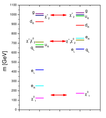
Figure 1: Illustration of the Flipper ambiguity in the MSSM spectrum. The left panel displays a typical mass value for the Bino, Wino, and Higgsino mixing parameter in the weak eigenstate basis for two models A and B. The right panel shows the corresponding sparticle spectrum in two of the AKTW models, with the red arrows indicating the Flipper effect.

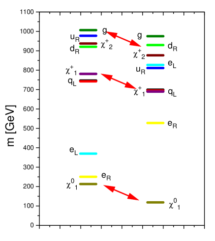
Figure 2: Illustration of the Slider ambiguity in the MSSM spectrum. The left panel displays a typical mass value for the Bino, Wino, and Higgsino mixing parameter in the weak eigenstate basis for two models A and B. The right panel shows the corresponding sparticle spectrum in two of the AKTW models, with the red arrows indicating the Slider effect.

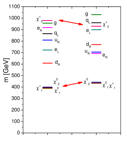
Figure 3: Illustration of the Squeezer ambiguity in the MSSM spectrum. The left panel displays a typical mass value for the Bino, Wino, and Higgsino mixing parameter in the weak eigenstate basis for two models A and B. The right panel shows the corresponding sparticle spectrum in two of the AKTW models, with the red arrows indicating the Squeezer effect.

One may wonder if there are any common features of these models that give rise to their indistinguishability at the LHC. AKTW demonstrated that these degeneracies are essentially the result of three possible characteristics that involve the relative composition of the physical electroweak gaugino sector in terms of the higgsino, wino, and bino weak eigenstates. These mechanisms are referred to as ‘Flippers’, ‘Sliders’ and ‘Squeezers’ and are schematically shown in Figs. 1, 2, and 3. The ambiguities that arise from these model characteristics originate directly from the manner in which SUSY is produced and observed at the LHC; several of these mechanisms can be simultaneously present. As is well-known, the (by far) dominant production mechanism for R-parity conserving SUSY at the LHC is via the strong interactions, i.e., the production of squarks and gluinos. These particles then decay through a long cascade chain via the generally lighter electroweak gaugino/higgsino partner states. This eventually leaves only the SM fields in the final state together with the stable Lightest SUSY Particle (LSP), which is commonly the lightest neutralino, appearing as additional missing energy. The decays of the SM fields produce additional jets, leptons, and missing transverse energy from neutrinos. Unfortunately sleptons do not always play a major role in these cascades (due to phase space considerations in the sparticle spectrum, see, e.g., the models in Fig. 1) so that much valuable information associated with their properties is generally lost. When comparing the possible decay chains which result from the produced squarks and gluinos, similar final states can occur if the identities of the higgsino, wino and bino weak states in the spectrum are interchanged while their masses are held approximately fixed. This is an example of the so-called ‘Flipper’ ambiguity (Fig. 1) where two spectra with interchanged electroweak quantum numbers can produce very similar final state signatures. A second possible source of degeneracy can arise from the fact that absolute masses, and in particular the mass of the LSP, are not well measured at the LHC in contrast to the mass differences between states Weiglein:2004hn ; Aguilar-Saavedra:2005pw . Thus models can have similar spectra but be somewhat off-set from each other in their absolute mass scale and hence be difficult to distinguish; this represents the ‘Slider’ degeneracy (Fig. 2). Lastly, pairs of states in the spectra with relatively small mass differences compared to the overall SUSY scale lead to relatively soft decay products in the cascade chain. Such a possibility can cause significant loss of information as well as general confusion in parameter extractions and are termed ‘Squeezers’ (Fig. 3). Of course in all these cases some shifts are needed in the strongly interacting part of the SUSY spectrum to keep the various production rates and decay distributions comparable between potentially indistinguishable models. It goes without saying that some degeneracies can also arise when more than one of these mechanisms are active simultaneously.

We now examine the physical particle spectra in the 383 models found by AKTW to be indistinguishable at the LHC. First, we note that since AKTW have required squarks and gluinos to have Lagrangian masses greater than 600 GeV in their parameter scans, the only states potentially accessible to the ILC will be the sleptons and the sparticles associated with the electroweak gaugino/higgsino sector. Of particular phenomenological interest is the mass splitting between the Next-to-LSP(NLSP) and LSP (see Fig. 4). Here, this is usually that between the lightest chargino, $\tilde{\chi}_{1}^{\pm}$, and lightest neutralino state, $\tilde{\chi}_{1}^{0}$. Generally this distribution for our set of AKTW models appears rather flat except for a huge and puzzling feature near $\sim 270$ MeV. It would seem that almost $40\%$, i.e., $141$ of these models, experience this exact mass splitting between these two states.

Final State	500 GeV	1 TeV
$\tilde{e}_{L}^{+}\tilde{e}_{L}^{-}$	9	82
$\tilde{e}_{R}^{+}\tilde{e}_{R}^{-}$	15	86
$\tilde{e}_{L}^{\pm}\tilde{e}_{R}^{\mp}$	2	61
$\tilde{\mu}_{L}^{+}\tilde{\mu}_{L}^{-}$	9	82
$\tilde{\mu}_{R}^{+}\tilde{\mu}_{R}^{-}$	15	86
Any selectron or smuon	22	137
$\tilde{\tau}_{1}^{+}\tilde{\tau}_{1}^{-}$	28	145
$\tilde{\tau}_{2}^{+}\tilde{\tau}_{2}^{-}$	1	23
$\tilde{\tau}_{1}^{\pm}\tilde{\tau}_{2}^{\mp}$	4	61
$\tilde{\nu}_{e\mu}\tilde{\nu}_{e\mu}^{*}$	11	83
$\tilde{\nu}_{\tau}\tilde{\nu}_{\tau}^{*}$	18	83
$\tilde{\chi}_{1}^{+}\tilde{\chi}_{1}^{-}$	53	92
Any charged sparticle	85	224
$\tilde{\chi}_{1}^{\pm}\tilde{\chi}_{2}^{\mp}$	7	33
$\tilde{\chi}_{1}^{0}\tilde{\chi}_{1}^{0}$	180	236
$\tilde{\chi}_{1}^{0}\tilde{\chi}_{1}^{0}$ only	91	0
$\tilde{\chi}_{1}^{0}+\tilde{\nu}$ only	5	0
$\tilde{\chi}_{1}^{0}\tilde{\chi}_{2}^{0}$	46	178
$\tilde{\chi}_{1}^{0}\tilde{\chi}_{3}^{0}$	10	83
$\tilde{\chi}_{2}^{0}\tilde{\chi}_{2}^{0}$	38	91
$\tilde{\chi}_{2}^{0}\tilde{\chi}_{3}^{0}$	4	41
$\tilde{\chi}_{3}^{0}\tilde{\chi}_{3}^{0}$	2	23
Nothing	61	3

Table 1: Number of models at $\sqrt{s}=500$ GeV and 1 TeV which have a given final state kinematically accessible. Note that for the 500 GeV case, 96/242 models have only LSP or neutral pairs accessible while 61/242 models have no SUSY particles accessible.

An investigation shows that this result is an artifact of the manner in which PYTHIA6.324 generates the physical SUSY particle spectrum at tree-level from the Lagrangian parameters. Recall that AKTW randomly generated points in a 15-dimensional weak scale MSSM parameter space, described in the previous Section, from which the physical SUSY particle masses are then calculated at tree-level via PYTHIA6.324. With this procedure, it is possible that sometimes the mass of the lightest chargino $\tilde{\chi}_{1}^{\pm}$ turns out to be less than that of the $\tilde{\chi}_{1}^{0}$ once the mass eigenstates are computed; this is usually considered to be ‘unphysical’ as it would imply charged Dark Matter in the standard cosmological picture. PYTHIA6.324 handles this situation by artificially resetting the chargino mass to be greater than that of the LSP by $m_{\tilde{\chi}_{1}^{\pm}}=m_{\tilde{\chi}_{1}^{0}}+2m_{\pi}$ without an associated warning message. This apparently happens frequently and causes the large peak in the distribution shown in Fig. 4. This feature is mentioned in the PYTHIA manual (where it is noted that the tree-level SUSY spectrum calculator is not for publication quality), and has been further clarified in later versions of PYTHIA peter . However, here we need to follow the analysis of AKTW as closely as possible to reproduce their sparticle spectra and specific model characteristics. Due to this and additional reasons discussed below in the text, in our analysis we use a slightly modified version of PYTHIA6.324. In the strictest sense, these models are only ‘unphysical’ at the tree-level since loop corrections restore the correct mass hierarchy. We have checked that all 383 of the AKTW models have an appropriate mass spectrum when the SuSpect2.34 routine suspectfolks , which includes the higher order corrections, is employed to generate the physical spectrum. However, in the present work, the 141 models cannot be artificially saved simply by employing this mass re-assignment or by using SuSpect as their collider production and signature properties would be modified as compared to the AKTW study. We thus drop them completely from further consideration. This leaves us with a sample of 242 models which consist of 162 degenerate model pairs to examine.

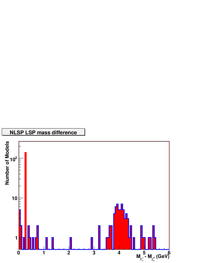
Figure 4: Low mass end of the lightest chargino-LSP mass difference which displays the PYTHIA feature in the sparticle spectrum generator discussed in the text.

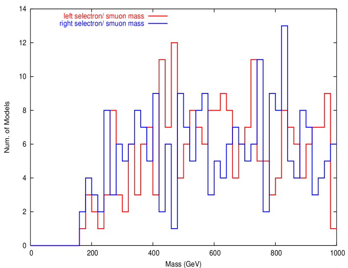
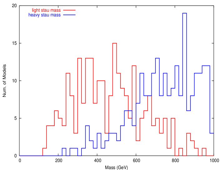
Figure 5: Selectron/smuon (top) and stau (bottom) mass spectra in the 242 models under study.

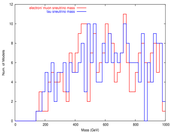
Figure 6: Sneutrino mass spectra in the 242 models under study.

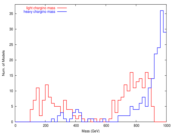
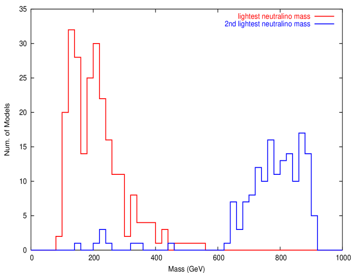
Figure 7: Chargino (top) and neutralino (bottom) mass spectra in the 242 models under study.

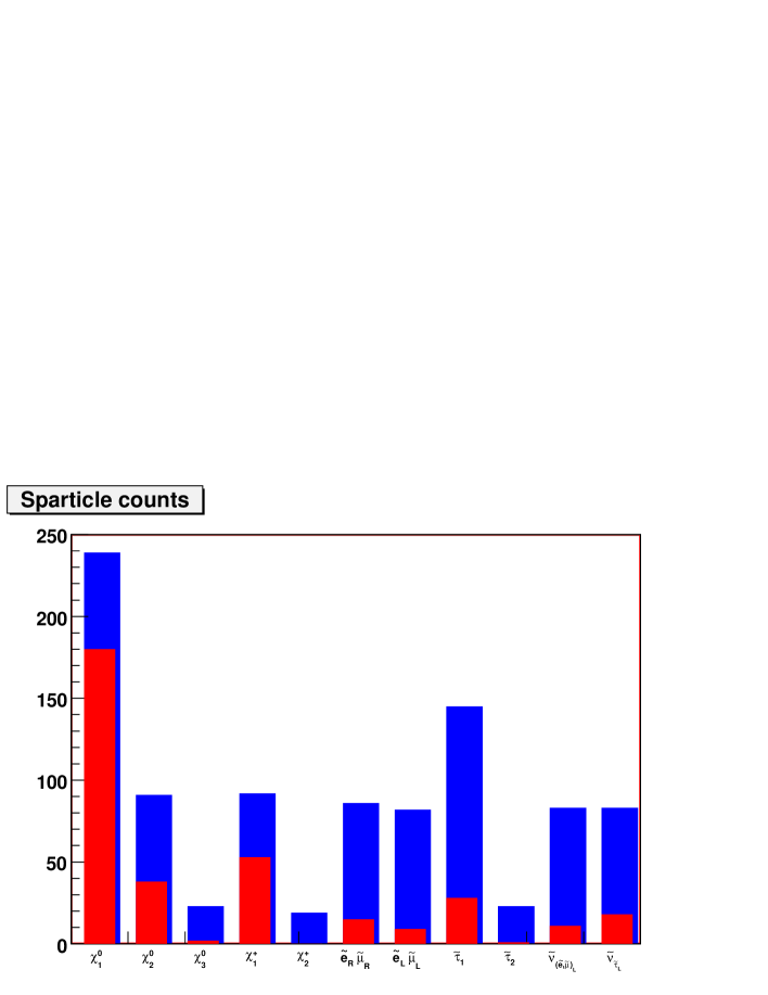
Figure 8: Number of models with various kinematically accessible MSSM states at a 500 (red) or 1000 (blue) GeV $e^{+}e^{-}$ collider via pair production.

Given these 242 models, we next address the question of what fraction of their SUSY spectra are kinematically accessible at a 500 or 1000 GeV ILC. The results are shown in Figs. 5, 6 and  7, which display the individual mass spectra for the weakly interacting sectors of the various SUSY models under consideration. The full accessible sparticle count for $\sqrt{s}=500$ and 1000 GeV is presented in Fig. 8. There are many things to observe by examining these Figures. First, we recall from the discussion above that in all cases the squarks are too massive to be pair produced at the ILC so that we are restricted to the slepton and electroweak gaugino sectors. Here in Table 1 and in the Figures we see that for a 500(1000) GeV collider, there are only 22(137)/242, i.e., 22(137) out of 242, models with kinematically accessible (which here means via pair production) selectrons and smuons at $\sqrt{s}=500(1000)$ GeV; note that these two sparticles are degenerate in the MSSM. Similarly, 28(145)/242 of the models have accessible light staus, 6(55) of which also have kinematically accessible selectrons/smuons. 53(92)/242 models have kinematically accessible light charginos, 4(12) of which also have accessible selectrons/smuons and 6(12) of which also have accessible staus. At $\sqrt{s}=1$ TeV, 19 of these 92 models with accessible light charginos also have the second chargino accessible by pair production. Very importantly, at $\sqrt{s}=500$ GeV, in 96/242 models the only kinematically accessible sparticles are neutral, e.g., $\tilde{\chi}_{1}^{0}$ or $\tilde{\nu}$, while 61/242 other models have no SUSY particles accessible whatsoever. At $\sqrt{s}=1$ TeV, these numbers drop to only 0/242 and 3/242 in each of these latter categories, respectively. Recalling that we are looking at essentially random points in the MSSM parameter space, we see from this simple counting exercise that $\sim 60\%$ of the models will have no ‘traditional’ SUSY signatures at a 500 GeV ILC, whereas a 1 TeV machine essentially covers almost all the cases. This is a strong argument for having the capability of upgrading to 1 TeV at the ILC as quickly as possible. However, in the analysis that follows we will consider only the case of a 500 GeV ILC with the 1 TeV case to be considered separately in the future. Table 1 summarizes the kinematic accessibility of all the relevant MSSM final states for $\sqrt{s}=500$ GeV in our study as well as the corresponding results for 1 TeV.

Given that so many models have such a sparse SUSY spectrum at $\sqrt{s}=500$ GeV, it is not uncommon for one of the two models in the pair we are comparing to have no kinematically accessible sparticles. In such a case, breaking the model degeneracy at the LHC might seem to be rather straightforward, as for one model we might observe SUSY signals above the SM background but not for the other in the pair. Of course, at the other end of the spectrum of difficulty, one can imagine cases where both models being compared are Squeezers, in which case model differentiation will be far more difficult and having an excellent ILC detector will play a much more important role.

III Analysis Procedure and General Discussion of Background

To determine whether or not the ILC resolves the LHC inverse problem, we compare the ILC experimental signatures for the pairs of SUSY models that AKTW found to be degenerate, and see whether these signatures can be distinguished. We examine numerous production channels and signatures for supersymmetric particle production in $e^{+}e^{-}$ collisions. Before the model comparisons can be carried out, we must first ascertain if the production of the kinematically accessible SUSY particles is visible above the SM background. Our analysis procedure is described in this Section.

III.1 Event Generation of Signal and Background

We generate 250 fb^-1 of SUSY events at $\sqrt{s}=500$ GeV for each of the AKTW models for both 80% left- and 80% right-handed electron beam polarization with unpolarized positron beams, providing a total of 500 fb^-1 of integrated luminosity. To generate the signal events, we use PYTHIA6.324 Sjostrand:2006za in order to retain consistency with the AKTW analysis. However, as will be described in detail below, we find that PYTHIA underestimates the production cross section in two of our analysis channels, and in these two cases we employ CompHEP Boos:2004kh . We also analyze two statistically independent 250 fb^-1 sets of Standard Model background events for each of the two electron beam polarizations. We then study numerous different analysis channels. When we determine if a signal is observable over the SM background in a particular channel, we statistically compare the combined distribution for the signal plus the background from our first background sample with the distribution from our second, independent background sample. When we perform the model comparisons, we add each set of SUSY events to a distinct Standard Model background sample generated for the same beam polarization. We then compare observables for the many different analysis channels for these two samples of signal and background (i.e., model A $+$ background sample 1 is compared to model B $+$ background sample 2). It is important to note that we take into account the full Standard Model background in all analysis channels rather than only considering the processes that are thought to be the dominant background to a particular channel; surprisingly, sometimes many small contributions can add up to a significant background.

Our background contains all SM $2\to 2$, $2\to 4$, and $2\to 6$ processes with the initial states $e^{+}e^{-}$, $e^{\pm}\gamma$, or $\gamma\gamma$; in total there are 1016 different background channels. These events were generated by T. Barklow TimB with O’MEGA as implemented in WHIZARD WHIZARD , which uses full tree-level matrix elements and incorporates a realistic beam treatment via the program GuineaPig Guinea . The use of full matrix elements leads to qualitatively different background characteristics in terms of both total cross section and kinematic distributions compared to those from a simulation that uses only the production and decay of on-shell resonances, e.g., the procedure generally employed in PYTHIA. WHIZARD models the flux of photons in $e^{\pm}\gamma$ and $\gamma\gamma$ initiated processes via the equivalent photon approximation. However, in the standard code, the electrons and positrons which emit the photon(s) that undergo hard scattering do not receive a corresponding kick in $p_{T}$, in contrast to the electrons or positrons that undergo initial state radiation. The version of WHIZARD used here to generate the background events was thus amended to correct this slight inconsistency in the treatment of transverse momenta. An illustration of the resulting effects from employing exact matrix elements and modelling the transverse momentum distributions in a realistic fashion is presented in Fig. 9. This Figure compares the transverse momentum distribution for the process $e^{+}e^{-}\rightarrow e^{+}e^{-}\nu_{e}\bar{\nu}_{e}$ in the SM after our selectron selection cuts (see Section 4.1) have been applied, as generated with PYTHIA versus the modified version of WHIZARD, using the same beam spectrum in both codes. We see that in this case, the $p_{T}$ distribution generated by PYTHIA is smaller and has a shorter tail.

e

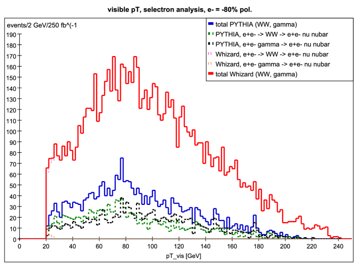
Figure 9: Transverse momentum distribution in $e^{+}e^{-}\to e^{+}e^{-}\nu_{e}\bar{\nu}_{e}$ as generated via PYTHIA and WHIZARD, for 250 fb^-1 of integrated luminosity with $80\%$ left-handed electron beam polarization at $\sqrt{s}=500$ GeV. Our selectron selection cuts (discussed in the text below) have been applied.

We now discuss our treatment of the beam spectrum in further detail. The backgrounds were generated using a realistic beam treatment, employing the program GuineaPig Guinea to model beam-beam interactions. Finite beam energy spread was taken into account and combined with a beamstrahlung spectrum specific to a cold technology linear collider, i.e., the ILC. The effect of beamstrahlung is displayed in Figure 10, which shows the invariant mass of muon pairs formed by $e^{+}e^{-}$ collisions with the beam spectrum we employ. The resulting spectrum is somewhat different qualitatively from a commonly used purely analytic approximate approach Yokoya:1989jb ; Chen:1991wd ; Peskin:1999pk .

Figure 10: Invariant mass of the muon pairs in $e^{+}e^{-}\rightarrow\mu^{+}\mu^{-}$ at $\sqrt{s}=500$ GeV, using the beamspectrum described in the text.

While our backgrounds contain 500 fb^-1 of total integrated luminosity for processes with initial $e^{+}e^{-}$ or $e^{\pm}\gamma$ states, some $\gamma\gamma$ initiated processes yield very high cross sections, and thus a smaller number of events had to be generated and then rescaled due to limited storage space. In total, our background sample uses approximately 1.7 TB of disk space. This rescaling of some $\gamma\gamma$ processes introduces artificially large fluctuations in the corresponding analysis distributions. In order to remedy this, we employ the following procedure: we combine the two independent background samples for the affected reactions, and then randomly reallocate each entry on a bin by bin basis to one of the two background sets. Thus, on average, each histogram contains an equal amount of entries bin per bin, while remaining statistically independent. Of course, this procedure does not completely eliminate the fluctuations. However, due to the random reallocation of entries, the contribution of these fluctuations to the statistical analyses in our comparison of models performed in Section 7 is greatly reduced.

III.2 Analysis Procedure

For each SUSY production process, we perform a cuts-based analysis, and histogram the distributions of various kinematic observables that we will describe in detail in the following Sections. We apply a general analysis strategy that performs uniformly well over the full MSSM parameter region. Each analysis is thus applied to every model in exactly the same fashion; there are no free parameters, and we do not make use of any potential information from the LHC; in particular we assume that the LSP mass is not known. Recall that the AKTW models that we have inherited are difficult cases at the LHC, and thus in general we cannot make any assumptions about what measurements, if any, will have been performed by the LHC detectors. We also note that AKTW did not impose any additional constraints from flavor physics, cosmological observations, etc. Such a global analysis is clearly desirable but is beyond the scope of the present study and is postponed to a future publication.

Our background and signal events described above are piped through a fast detector simulation using the org.lcsim detector analysis package lcsim , which is currently specific to the SiD detector design SiD . org.lcsim is part of the Java Analysis Studio (jas3) jas3 , a general purpose java-based data analysis tool. The org.lcsim fast detector simulation incorporates the specific SiD detector geometry, finite energy resolution, acceptances, as well as other detector specific processes and effects. Unfortunately, the identification of displaced vertices and a measurement of dE/dx are not yet implemented in the standard, fully tested version of the simulation package employed here, although preliminary versions of these functions are under development. The present study represents the first large end user application of the lcsim software package and hence we prefer to use the standard, tested, version of the software without these additional features. The output of our lcsim-based analysis code is given in terms of AIDA histograms, where AIDA refers to Abstract Interfaces for Data Analysis Serbo:2003sm , a standard set of java and C++ interfaces for creating and manipulating histograms, which is incorporated into the jas3 framework.

org.lcsim allows for the study of various different detectors, whereby an xml description of the specific detector is loaded into the software in a modular fashion. Currently, xml descriptions for various slightly different versions of the SiD detector geometry are publicly available. We use the SiD detector version studied extensively at Snowmass 2005 (sidaug05) snowmass . In addition, two files, called ClusterParameters.properties and TrackingParameters.properties allow the user to adjust various tracking and energy resolution parameters. We set the parameters such that we closely follow the SiD detector outline document (DOD) SiDDOD . In particular, we employ the following configuration in our study:

• The minimum transverse momentum of registered tracks is given by $p_{T}>0.2$ GeV.

• There is no tracking capability below 142 mrad, which corresponds to $\left|\cos\theta\right|<0.99$.

• Between 142 mrad and 5 mrad, electromagnetically charged particles appear as neutral clusters.

• There is no detector coverage below 5 mrad.

• The jet energy resolution is set to $30\%/\sqrt{E}$.

• The electromagnetic energy resolution is set to $18\%/\sqrt{E}$.

• The hadronic energy resolution is set to $50\%/\sqrt{E}$.

• The hadronic degradation fraction is $r=1.0$.

• The electromagnetic jet energy fraction is $w_{\gamma}=0.28$.

• The hadronic jet energy fraction is $w_{h}=0.1$.

For a detailed explanation of these parameters we refer to the SiD DOD, specifically Section IV.B regarding the energy resolution parameters.

However, we note that the lack of tracking capability below 142 mrad causes highly energetic forward muons to not be reconstructed. They are too energetic to deposit energy into clusters and are thus undetected and appear as missing energy. This effect produces a substantial Standard Model background to, e.g., our stau analysis (see Section IV.1.3), where we allow one tau to decay hadronically and the other leptonically. In this case, we keep events with one electron and one muon of opposite charge, which can be mimicked by $\gamma\gamma\rightarrow\mu^{+}\mu^{-}$ events where one of the beam electrons is kicked out sufficiently to be detected, but one of the final state muons is too energetic and too close to the beam axis to be reconstructed. We find that this background is substantial and, given these detector parameters, can only be eliminated by discarding all tau events with electrons/positrons in the final state.

The default jet finding algorithm of org.lcsim is the JADE jet algorithm Bethke:1988zc in the E scheme with $y_{\mbox{\tiny cut}}=0.005$ employed as the default setting. The JADE jet algorithm in the E scheme is defined as follows:

$$\min\left(p_{i}+p_{j}\right)^{2}\! = \!\min 2E_{i}E_{j}(1-\cos\theta_{ij})>y_{\mbox{\tiny cut}}s$$ (1)

$$p_{ij}=p_{i}+p_{j}$$ for the recombination scheme

The default $y_{\mbox{\tiny cut}}$, however, is too small, and causes soft gluons to produce far too many jets. We therefore set the value of $y_{\mbox{\tiny cut}}$ to $y_{\mbox{\tiny cut}}=0.05$ within the JADE jet algorithm. In addition, one must take care when using the default org.lcsim jet finder, as every parton, including leptons and photons, is in principle identified as a jet. More sophisticated jet finders are in the development stage. We thus use the default jet finder, but with additional checks on the jet particle content to discard non-hadronic “jets”.

We perform searches for slepton, chargino, and neutralino production and in many cases design analyses for several different decay channels of these sparticles. Each of our analyses is designed to optimize a particular signature, and we apply each analysis to every AKTW model. A particular model may or may not produce a visible signature in a specific channel. We will describe our cuts in detail for each analysis channel in the Sections below.

As a starting point, we incorporate sets of kinematic cuts that were developed in various previous supersymmetric studies in the literature (the specific references are given in the following Sections). However, in many cases we find that some of these cuts are optimized for specific Supersymmetry benchmark points, e.g., the Snowmass Points and Slopes (SPS) Aguilar-Saavedra:2005pw , and are too stringent for the general class of models we study here. In other cases, we find that the cuts employed in the literature are not stringent enough to sufficiently reduce the Standard Model background in order to obtain a good signal to background ratio. Through a seemingly endless series of iterations, we have thus designed sets of cuts (which are described in the following Sections) that optimize the signal to background ratio for an arbitrary point in MSSM parameter space. This scenario corresponds to a first sweep of ILC data in search of a SUSY signal, and is therefore a reasonable course of action. We also remind the reader that these AKTW models are difficult at the LHC and hence the slepton, chargino, and neutralino states will not necessarily be observable at the LHC.

The signatures that we have developed analyses for are summarized in Table 2, which lists the signature, dominant background source, and the observable kinematic distribution for each SUSY production process. We note that in some cases, the same signature can arise from different sources of sparticle production, e.g., $\mu^{+}\mu^{-}+$ missing energy can occur from both smuon and chargino production. Indeed, it is well known that sometimes SUSY is its own background and we will note this in the following Sections. Our cuts, however, are chosen such to minimize this effect.

Sparticles Produced	Signature	Main Background	Observable
$\tilde{e}^{+}\tilde{e}^{-}$	$e^{+}e^{-}$ + missing E	$e^{+}e^{-}\rightarrow e^{-}\bar{\nu}_{l}\nu_{l}{e}^{+},\,$	energy of $e^{+},\,e^{-}$
$\tilde{\mu}^{+}\tilde{\mu}^{-}$	$\mu^{+}\mu^{-}$ + missing E	$e^{+}e^{-}\rightarrow\mu^{-}\bar{\nu}_{l}\nu_{l}{\mu}^{+},\,$	energy of $\mu^{+},\,\mu^{-}$
$\tilde{\tau}^{+}\tilde{\tau}^{-}$	$\tau^{+}\tau^{-}$ + missing E	$e^{\pm}\gamma\rightarrow e^{\pm}\nu\bar{\nu}$	energy of tau jets
		$e^{\pm}\gamma\rightarrow e^{\pm}l^{+}l^{-}$
$\tilde{\nu}\tilde{\nu}^{*}$	$jjjjl^{+}l^{-}$ + missing E	$\gamma\gamma\rightarrow c\bar{c},b\bar{b}$	missing energy
$\tilde{\nu}\tilde{\nu}^{*}$	$jjjjjj$ + missing E	none	missing energy
$\tilde{\chi}^{+}_{1}\tilde{\chi}^{-}_{1}$	$\mu^{+}\mu^{-}$ + missing E	$e^{+}e^{-}\rightarrow l^{-}\bar{\nu}_{l}\nu_{l^{\prime}}{l^{\prime}}^{+}$	energy of $\mu^{+},\,\mu^{-}$
$\tilde{\chi}^{+}_{1}\tilde{\chi}^{-}_{1}$	$jj\mu^{\pm}$ + missing E	$e^{+}e^{-}\rightarrow q\bar{q}^{\prime}l\bar{\nu}_{l}$	energy and invariant
		$\gamma\gamma\rightarrow\tau^{+}\tau^{-}$	mass of dijet pair
		$\gamma\gamma\rightarrow q\bar{q}$
$\tilde{\chi}^{+}_{1}\tilde{\chi}^{-}_{1}$	$jjjj$ + missing E	$\gamma\gamma\rightarrow q\bar{q}$	energy and invariant
			mass of dijet pairs,
			missing energy
$\tilde{\chi}^{+}_{1}\tilde{\chi}^{-}_{1}$	$\gamma$ + charged tracks	$e^{+}e^{-}\rightarrow l^{-}\bar{\nu}_{l}\nu_{l^{\prime}}{l^{\prime}}^{+}$	recoil mass
		$e^{\pm}\gamma\rightarrow e^{\pm}l^{+}l^{-}$
$\tilde{\chi}^{+}_{1}\tilde{\chi}^{-}_{1}$ or $\tilde{\tau}^{+}\tilde{\tau}^{-}$	2 stable charged tracks	$e^{+}e^{-}\rightarrow e^{+}e^{-}+\mbox{ISR,BS}$	$p/E$
$\tilde{\chi}^{0}_{2}\tilde{\chi}^{0}_{1}$	$l^{+}l^{-}$ + missing E	$\gamma\gamma\rightarrow l^{+}l^{-}$	invariant mass
			of lepton pair
$\tilde{\chi}^{0}_{2}\tilde{\chi}^{0}_{1}$	$jj$ + missing E	$e^{\pm}\gamma\rightarrow\nu_{e}q\bar{q}$	invariant mass
			of jet-pair
$\tilde{\chi}^{0}_{1}\tilde{\chi}^{0}_{1}$	$\gamma$ + nothing	$e^{+}e^{-}\rightarrow\gamma\nu\bar{\nu}$	photon energy

Table 2: Summary of signatures and observables in all analysis channels that we study and sources of the main standard model background. $l=e,\mu,\tau$

As discussed in the introduction, the first step in our analysis is to determine whether or not a given SUSY particle is visible above the SM background. Specifically, for a kinematic distribution resulting from our analysis of a given observable, we ask whether or not there is sufficient evidence to claim a ‘discovery’ for a SUSY particle within a particular model. There are many ways to do this, but we follow the Likelihood Ratio method, which we base on Poisson statistics. (See, e.g., Ref. Ball:2007zz ). In this method, we introduce the general Likelihood distribution:

$$L(n,\mu)=\prod_{i}^{bins}{{\mu_{i}^{n_{i}}e^{\mu_{i}}}\over{n_{i}!}}\,,$$ (2)

where $n_{i}(\mu_{i})$ are the number of observed (expected) events in each bin $i$ and we take the product over all the relevant bins in the histogram. As discussed above, we have generated two complete and statistically independent background samples, which we will refer to as $B1$ and $B2$. Combining the pure signal events, $S$, which we generate for any given model with one of these backgrounds, we form the Likelihood Ratio

$$R=L(S+B1,B2)/L(B1,B2)\,.$$ (3)

The criterion for a signal to be observed above background is that the significance, $\cal S$, satisfy

$${\cal S}=\sqrt{2\log R}>5\,.$$ (4)

This corresponds to the one-sided Gaussian probability that a fluctuation in the background mimics a signal of $\simeq 2.9\cdot 10^{-7}$, which is the usual $5\sigma$ discovery criterion. When employing this method, we sometimes encounter bins within a given histogram for which there is no background due to low statistics but where a signal is observed. In this case, the function $L$ is not well-defined. When this occurs we enter a single event into the empty background histogram in that bin.

Given that our full SM background samples are only available at fixed energies, our toolbox does not include the ability to do threshold scans. As is well known, this is a very powerful technique that can be used to obtain precision mass determinations for charged SUSY (or any other new) particles that are kinematically accessible. Such measurements would certainly aid in the discrimination between models, especially in difficult cases where the measurements we employ do not suffice. In addition, especially for sparticles which decay inside the detector volume, input from the excellent SiD vertex detector could prove extremely useful. In the analysis presented below, the vertex detector is used only for track matching and not as a search tool for long-lived states.

IV Slepton Production

IV.1 Charged Slepton Pair Production

For detecting the production of charged sleptons, we focus on the decay channel

$$\tilde{l}^{+}\tilde{l}^{-}\rightarrow l^{+}l^{-}\tilde{\chi}^{0}_{1}\tilde{\chi}^{0}_{1}\,,$$ (5)

that is, the signature is a lepton pair plus missing energy. In the cases of selectrons and smuons these signatures are fairly straightforward to study; the stau case is slightly more complicated due to the more involved tau identification.

As is well known, the main Standard Model background for all of these cases arises from the production of $W$ pairs followed by their subsequent decay into lepton-neutrino pairs and from $Z$-boson pair production, where one $Z$ decays into a charged lepton pair and the other into a neutrino pair. A significant background also arises from gamma-induced processes through beam- and bremsstrahlung.

The $W$ pair background produces leptons that are predominantly along the beam axis towards $|\cos\theta|\approx 1$, where $\theta$ takes on the conventional definition. This is because the decaying $W$ bosons are produced either through $s$-channel $Z$- or $\gamma$-exchange, for which the differential cross section is proportional to $(1+\cos^{2}\theta)$, or through $t$-channel neutrino-exchange, which behaves as $1/\sin^{4}(\theta/2)$. The photon-induced background also yields electrons that are peaked along the beam axis because they are mainly produced at low $p_{T}$ from beam- and bremsstrahlung, although our more realistic beamspectrum has a larger $p_{T}$ tail than the PYTHIA-generated backgrounds studied conventionally (cf. the discussion in Sec. III). As we will illustrate below in Section 4.1.3, having the best possible forward detector coverage in terms of tracking and particle identification (ID) is therefore of utmost importance to reduce the Standard Model background.

To reduce the SM background, we employ a series of cuts that have been adapted and expanded from previous studies Goodman ; Martyn:2004jc ; Bambade:2004tq . Our cuts are fairly similar for all slepton analyses. We will discuss them in detail in our selectron analysis presented below, and then will list the cuts with only brief comments in our discussion of smuon and stau production.

IV.1.1 Selectrons

As discussed above, in the case of selectron production we study the clean decay channel

$$\tilde{e}^{+}\tilde{e}^{-}\rightarrow e^{+}e^{-}\tilde{\chi}^{0}_{1}\tilde{\chi}^{0}_{1}\,,$$ (6)

that is, the signature is an electron pair plus missing energy. The main backgrounds arising from the SM originate in $W$ and $Z$ pair production, followed by their leptonic decays, along with several processes originating from both $\gamma\gamma$ and $\gamma e$ interactions. To reduce these backgrounds we employ the following cuts, which are expanded from those in Goodman :

1. We require exactly two leptons, identified as an electron and a positron, in the event and that there be no other charged particles. This removes SM backgrounds where, for example, both $Z$ bosons decay into charged leptons.

2. $E_{\mbox{\tiny vis}}<1$ GeV for $|\cos\theta|\geq 0.9$, where $E_{\mbox{\tiny vis}}$ corresponds to the visible energy in the event. This helps to reduce large SM background from forward $W$ production, as well as beam-/bremsstrahlung reactions that yield leptons predominantly along the direction of the beam axis.

3. $E_{\mbox{\tiny vis}}<0.4\sqrt{s}$ in the forward hemisphere. Here, the forward hemisphere is defined as the hemisphere around the thrust axis which has the greatest visible energy. Since we only have 2 visible particles in the final state, this amounts to defining the forward hemisphere about the particle with the highest energy. The SUSY signal has missing energy in both hemispheres, whereas the SM reaction $e^{+}e^{-}\to ZZ\to e^{+}e^{-}\nu\bar{\nu}$ has missing energy in only one of the hemispheres since the decay $Z\to\nu\bar{\nu}$ occurs in the hemisphere opposite of the $Z$ decay to charged leptons.

4. The angle between the reconstructed electron-positron pair is restricted to have $\cos\theta>-0.96$. Since SUSY has a large amount of missing energy, the selectron pair will not be back-to-back, in contrast to the SM background events.

5. We demand that the visible transverse momentum, or equivalently, the transverse momentum of the electron-positron pair, $p_{T\mbox{\tiny vis}}=p_{T}^{\,e^{+}e^{-}}>0.04\sqrt{s}$. This cut significantly reduces both the $\gamma\gamma$ and $e^{\pm}\gamma$ backgrounds which are mostly at low $p_{T}$.

6. The acoplanarity angle must satisfy $\Delta\phi^{e^{+}e^{-}}>40$ degrees. Since we demand only an electron and positron pair, the acoplanarity angle is equivalent to $\pi$ minus the angle between the transverse momentum of the electron and positron, $\Delta\phi^{e^{+}e^{-}}=\pi-\theta_{T}$. This requirement translates to a restriction on the transverse angle of $\cos\theta_{T}>0.94$. This cut further reduces contributions from both the $W$-pair and $\gamma\gamma$ backgrounds where the $e^{+}e^{-}$ pair tends to be more back-to-back.

7. $M_{e^{+}e^{-}}<M_{Z}-5\mbox{ GeV}$ or $M_{e^{+}e^{-}}>M_{Z}+5\mbox{ GeV}$, where $M_{e^{+}e^{-}}$ is the invariant mass of the lepton pair. This cut is to further remove events from $Z$ boson pair production with subsequent decays into $e^{+}e^{-}$ pairs.

As already mentioned above, we note that below 142 mrad ($\left|\cos\theta\right|>0.99$), the SiD detector does not have particle tracking information according to the current detector design SiDDOD , and any charged particle in this region appears only as a neutral electromagnetic cluster. However the first cut listed above, where we demand exactly an $e^{+}e^{-}$ pair in the final state, substitutes for potentially more detailed cuts that assume tracking capabilities down to much smaller angles.

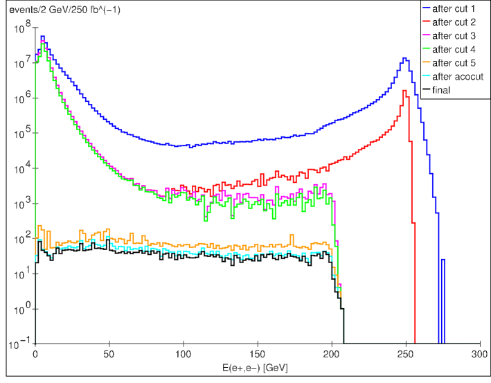
Figure 11: Standard Model background after each of the cuts listed in the text is successively imposed for an incoming right-handed electron beam with 80% polarization and $250\mbox{ fb}^{-1}$ of integrated luminosity.

The standard selectron search analysis is based on the energy distribution of the final state electron or positron. Since the selectron decays into a clean 2-body final state, the $e^{-}/e^{+}$ energy distribution has a box-shaped “shelf” in a high statistics, background-free, perfect detector environment in the absence of radiative effects. Kinematics determines the minimum and maximum electron energies which are related to the two unknown masses of the selectron and LSP by

$$E_{\max} = \frac{\sqrt{s}}{4}\left(1+\sqrt{1-\frac{4m_{\tilde{e}}^{2}}{s}}\right)\left(1-\frac{m_{\tilde{\chi}^{0}_{1}}^{2}}{m_{\tilde{e}}^{2}}\right)\,,$$ (7)

$$E_{\min} = \frac{\sqrt{s}}{4}\left(1-\sqrt{1-\frac{4m_{\tilde{e}}^{2}}{s}}\right)\left(1-\frac{m_{\tilde{\chi}^{0}_{1}}^{2}}{m_{\tilde{e}}^{2}}\right)\,.$$ (8)

The sharp edges of this box-shaped energy distribution allow for a precise determination of the selectron and LSP masses. However, due to beamstrahlung, the effective $\sqrt{s}$ above will vary, and once detector effects are also included the edges of this distribution will tend to be slightly washed out. Since our goal here is to simply detect superpartners and then distinguish models with different sets of underlying parameters, we do not need to perform a precise mass determination in the present analysis. We also consider additional kinematic observables, such as the distribution of $p_{T}^{vis}$ and the $e^{+}e^{-}$ invariant mass $M_{ee}$, as they will be useful at separating different SUSY signal sources.

The successive effect of each of the above cuts on the SM background is illustrated in Fig. 11. Here, we show the electron and positron energy distribution for 250 $\mbox{fb}^{-1}$ of simulated Standard Model background for RH electron beam polarization at $\sqrt{s}=500\,$ GeV. The $y$-axis corresponds to the number of events per 2 GeV bin. We note that cuts number 1-5 essentially eliminate any potential background arising from the large Bhabha scattering and $\gamma\gamma\rightarrow e^{+}e^{-}$ cross sections. The main contribution to the background remaining after these cuts arises from processes involving $W$ and $Z$ pair production from electron positron initial states, i.e., $e^{+}e^{-}\to\ell^{-}\bar{\nu}_{\ell}\nu_{\ell^{\prime}}{\ell^{\prime}}^{+}$, with $\ell^{(^{\prime})}=e,\tau$, as shown in Fig. 12. We find that most of the photon initiated background has been removed by our cuts. Note that applying these cuts in a different order would necessarily show a different level of effectiveness.

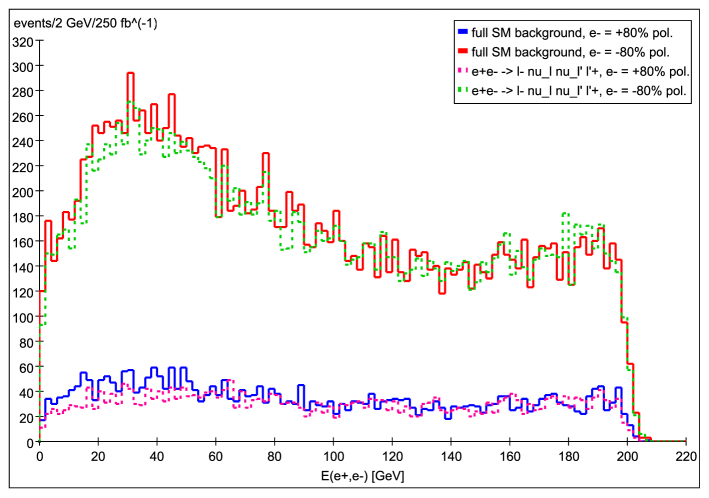
Figure 12: Remaining SM background after the full set of selectron selection cuts listed in the text are imposed. This is generated from $250\mbox{ fb}^{-1}$ of SM events with 80% right-handed (solid blue line) and 80% left-handed (solid red line) electron beam polarization, and unpolarized positron beam at $\sqrt{s}=500$ GeV. The dotted lines show the main process contributing to the background, $e^{+}e^{-}\rightarrow\ell^{-}\bar{\nu}_{\ell}\nu_{\ell^{\prime}}{\ell^{\prime}}^{+}$, with $\ell^{(^{\prime})}=e,\tau$, for 80% right-handed (dotted pink line) and 80% left-handed (dotted green line) electron polarization. Note that here and in other Figures below the spikes in the full background and the main contributions are because of rescaling issues and the thus necessary mixing of the two independent background samples (cf. the discussion in Section 3.1). This mixing is a random procedure which explains why the spikes are not all in the same bins.

A further comment on cut number 5 is in order. One finds that increasing this cut from $p_{T}^{\,e^{+}e^{-}}>20$ GeV to $p_{T}^{\,e^{+}e^{-}}>30$ GeV at $\sqrt{s}=500$ GeV to further reduce the photon initiated background, introduces a dip in the center of the “shelves” for MSSM models that have edges near $E_{e}\simeq$ 30-40 GeV. This apparently occurs when both visible leptons have approximately the same amount of energy, so that their transverse momenta partially cancel, leaving insufficient visible transverse momentum to pass the cut. When one of the leptons is more energetic than the other, the visible $p_{T}$ is generally above the cut. Thus increasing the cut on visible $p_{T}$ in order to reduce the background further also affects the signal in a perhaps somewhat unexpected way. The same observation also applies in the smuon analysis below.

Figure 13 shows how a typical signal from a model with kinematically accessible selectrons responds to the same cuts that were applied to the backgrounds above. Note that while the cuts reduce the backgrounds by many orders of magnitude, the signal is reduced only by a factor of $2-3$.

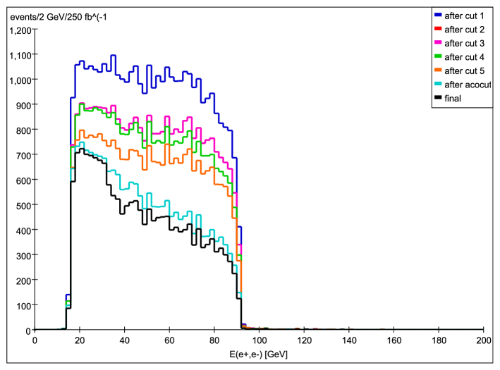
Figure 13: The electron energy distribution for selectron production after successively imposing each of the cuts listed in the text for the case of a right-handed incoming electron beam with 80% polarization and 250 fb^-1 of integrated luminosity.

We now examine selectron pair production for the AKTW models. In this case, there are 22/242 (22 out of 242) models with kinematically accessible selectrons at $\sqrt{s}=500$ GeV. The $\tilde{e}_{L(R)}$ is accessible in 9(15) of these 22 models; for 2 models we find that both states are potentially visible. Note that fewer than $10\%$ of our models have this relatively clean channel accessible. Selectrons are pair produced via $s$-channel $\gamma$ and $Z$ exchange as well as $t$-channel neutralino exchange. For the case of the well-studied $\tilde{e}\to e\tilde{\chi}_{1}^{0}$ decay mode, which we examine here, selectrons are usually searched for by examining the detailed structure of the resulting individual $e^{\pm}$ energy spectra and looking for any excesses above the expected SM background. As is by now well-known and briefly discussed above, in the absence of such backgrounds, with high statistics and neglecting any radiative effects, the 2-body decay of the selectrons lead to flat, horizontal shelves in this distribution. In a more realistic situation where all such effects are included and only finite statistics are available, the general form of the shelf structure remains but they are now jagged, tilted downwards (towards higher $e^{\pm}$ energies), and have somewhat smeared edges. These effects are illustrated in Fig. 14 which shows examples of the $e^{\pm}$ spectra (adding signal and background) for some representative AKTW models containing kinematically accessible selectrons with either beam polarization configuration. There are several important features to note in these Figures. The detailed nature of the $\tilde{e}$ signal in the $e^{\pm}$ energy spectrum shows significant variation over a wide range of both magnitude and width depending upon the $\tilde{e}_{L,R}$ and $\tilde{\chi}_{1}^{0}$ masses and the resulting production cross sections. Recall that $t$-channel sneutrino exchange can be important here and dramatically affects the size of this cross section. The ratio of signal to background is not always as large as in most cases discussed in the literature. In addition, we note that the range of possible signal shapes relative to the SM background can be varied; not all of our signals appear to be truly shelf-like. In some models, the background overwhelms the signal. Note that RH polarization leads to far smaller backgrounds than does LH polarization as would be expected, this being due to the diminished contribution from $W$-pairs which prefer LH coupling.

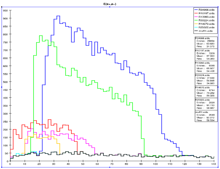
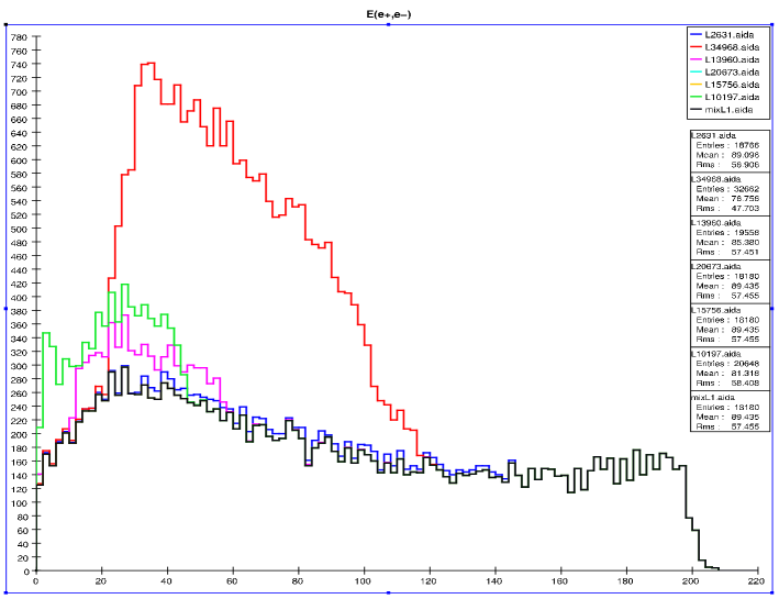
Figure 14: Electron energy distribution: the number of events/2 GeV bin after imposing the full set of cuts discussed in the text for several representative models. RH(LH) beam polarization is employed in the top(bottom) panel, assuming $80\%$ electron beam polarization an integrated luminosity of 250 fb^-1 for either polarization. The SM background is shown as the black histogram.

Of the 22 kinematically accessible models, 18(15) lead to signals with a visibility significance over background of ${\cal S}>5$ at these integrated luminosities assuming RH(LH) beam polarization. Combining the LH and RH polarizations channels we find that 18/22 models with selectrons lead to signals with significance $>5$. Furthermore, $8/9$ models with kinematically accessible $\tilde{e}_{L}$ are observable while $12/15$ models with $\tilde{e}_{R}$ are visible. Note that 4 models have selectrons with masses that are in excess of 241 GeV. This leads to a strong kinematic suppression in their cross sections and, hence, very small signal rates, so they are missed by the present analysis. Some of the models in both the RH and LH polarization channels have a rather small $S/B$ and are not easily visible at this level of integrated luminosity; typical examples of ‘difficult’ models are presented in Figs. 15 and  16.

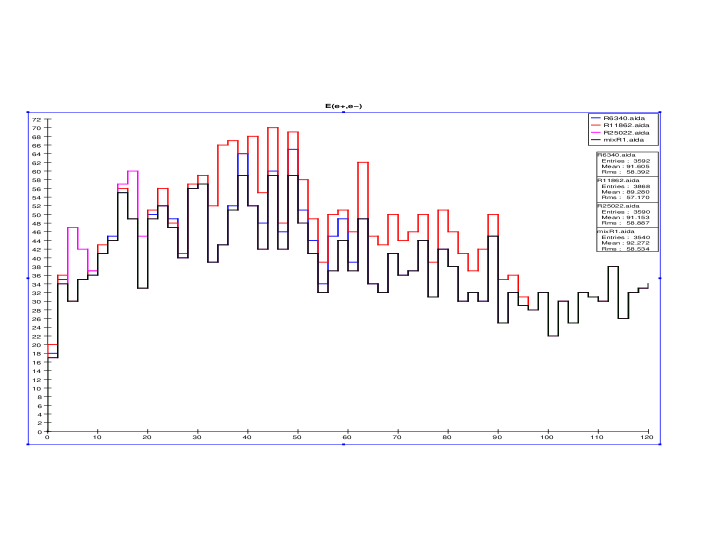
Figure 15: Same as the previous Figure but now for three models which are difficult to observe due to small cross sections in the RH polarization channel.

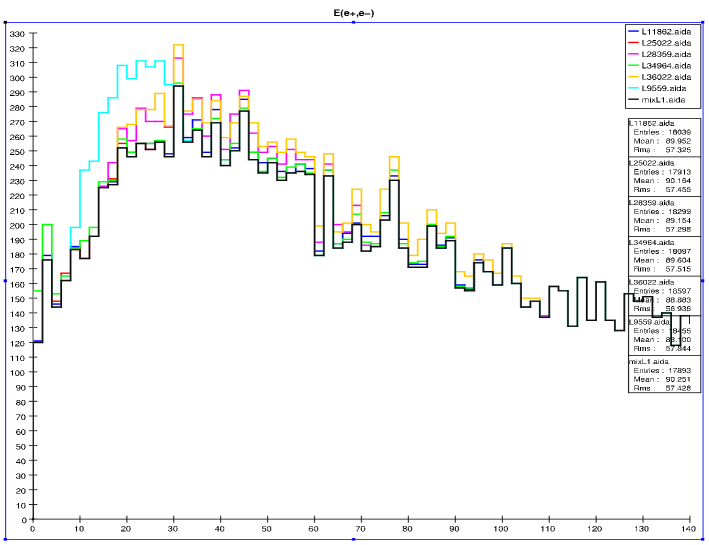
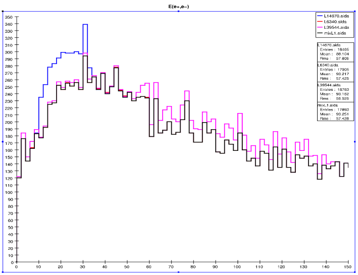
Figure 16: Same as the previous Figure but now for the LH polarization channel for two sets of models which are a bit more difficult to observe due to small cross sections.

It is interesting to compare these results to what we obtain in the case of the well-studied SPS1a’ benchmark model Aguilar-Saavedra:2005pw ; Fig. 17 shows the electron energy distribution for this model for both beam polarization choices in an analogous manner to that shown in the previous Figures for the AKTW models. Due to the large production cross section, detecting the signal in this case is rather trivial as we would expect from the detailed studies made in the literature. The most important thing to notice from this Figure is that SPS1a’ leads to substantially larger signal rates than in any of the models we are investigating in the present analysis. In fact, the SPS1a’ signal rates can be almost two orders of magnitude larger than some of the models we are examining here. We also observe the obvious presence of two shelves, especially in the case of LH beam polarization, clearly indicating that both the $\tilde{e}_{L}$ and $\tilde{e}_{R}$ states are kinematically accessible and are being simultaneously produced.

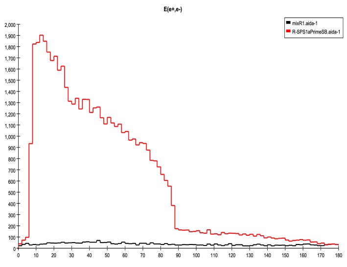
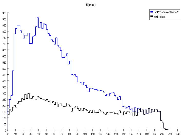
Figure 17: The electron energy distribution after imposing the full set of cuts discussed in the text for the benchmark model SPS1a’. RH(LH) beam polarization is employed in the top(bottom) panel, assuming an integrated luminosity of 250 fb^-1 for either polarization. The SM background is shown as the black histograms.

Interestingly, one finds that there are a number of models, particularly in the case of RH polarization, which do not have kinematically accessible selectrons but which have visible signatures in the $\tilde{e}$-pair analysis. This is an example of SUSY being a background to SUSY. There are, of course, other SUSY particles which can decay into $e^{\pm}$ and missing energy, e.g., chargino pair production followed by the decay $\tilde{\chi}_{1}^{+}\to W^{*}\tilde{\chi}_{1}^{0}$ with $W^{*}\to e\nu$, or associated $\tilde{\chi}_{2}^{0}\tilde{\chi}_{1}^{0}$ production followed by the decay $\tilde{\chi}_{2}^{0}\to e^{+}e^{-}\tilde{\chi}_{1}^{0}$. Both of these processes result in the same observable final state. Figure 18 shows some of these ‘fake’ models that appear in our selectron analysis in the case of RH polarization. Fake models, by which we mean models where other SUSY particle production leads to a visible signature in the selectron analysis, also appear for LH polarization and, in fact, we find 14 counterfeit models for either polarization. Note that the shapes of these fake model signatures are somewhat different than those in a typical model with actual selectrons present; there are no truly shelf-like structures and the $e^{\pm}$ energies are all peaked at relatively low values. This occurs because in these examples the final state electrons are the result of a 3-(or more) body decay channel when the $W$ boson is off-shell and because the $\tilde{\chi}_{1}^{\pm}-\tilde{\chi}_{1}^{0}$ mass splitting is relatively small. Both of these conditions are present in most of our models.

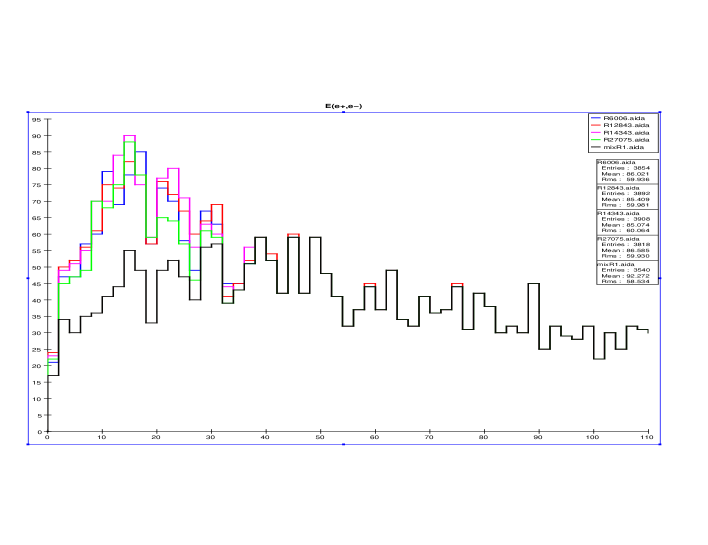
Figure 18: The electron energy distribution after imposing the full set of cuts discussed in the text for a subset of fake selectron models in the RH polarization channel. The SM background is shown as the black histogram as usual.

If further differentiation from the fake signatures is required, we need to examine a different kinematic distribution, e.g., the invariant mass of the $e^{+}e^{-}$ pair, $M_{ee}$. One would expect the counterfeit signals to populate small values of $M_{ee}$ while the models with actual selectrons will have a higher number of events with larger values of $M_{ee}$. This is indeed the case as can be clearly seen in Fig. 19. As we will see below, fake signals occur quite commonly in almost all of our analyses. Though specific analyses are designed to search for a particular SUSY partner it is quite easy for other SUSY states to also contribute to a given final state and be observed instead, e.g., a similar signature can be generated using the visible $p_{T}$ of the electron.

It would be interesting to return to this issue with a wider set of models that lead to larger mass splittings in the electroweak gaugino sector to see how well selectrons and charginos can be differentiated under those circumstances.

Figure 19: The dielectron invariant mass spectrum in the RH polarization channel for true selectron models (top) and those caused by other SUSY particles (bottom).

IV.1.2 Smuons

For $\tilde{\mu}$ pair production the standard search/analysis channel is

$$\tilde{\mu}^{+}\tilde{\mu}^{-}\rightarrow\mu^{+}\mu^{-}\tilde{\chi}^{0}_{1}\tilde{\chi}^{0}_{1}\,,$$ (9)

i.e., the signature is a muon pair plus missing energy. Smuon production occurs via $s$-channel $\gamma$ and $Z$ exchange; there is no corresponding $t$-channel contribution as in the case of selectrons. As in the selectron analysis, the dominant background arises from leptonic decays of $W$-pair and $Z$-pair production, as well as the ubiquitous (though somewhat less important in this case) $\gamma\gamma$ background. Since the background and signal are similar to those for selectron production, our choice of cuts here will follow those employed in the selectron analysis above and are adapted from those proposed by Martyn Martyn:2004jc (see also Bambade:2004tq ):

1. No electromagnetic energy (or clusters) $>0.01\sqrt{s}$ in the region $|\cos\theta|>0.995$.

2. Exactly two muons are in the event with no other charged particles and they are weighted by their charge within the polar angle $-0.9<Q_{\mu}\cos\theta_{\mu}<0.75$ with no other visible particles. This removes a substantial part of the $W$-pair background.

3. The acoplanarity angle satisfy $\Delta\phi^{\mu\mu}>40$ degrees. This reduces both the $W$-pair and $\gamma\gamma$ backgrounds.

4. $|\cos\theta_{p_{\mbox{\tiny}missing}}|<0.9$.

5. The muon energy is constrained to be $E_{\mu}>0.004\sqrt{s}$.

6. The transverse momentum of the dimuon system, or equivalently, visible transverse momentum (since only the muon pair is visible), satisfy $p_{T\mbox{\tiny vis}}=p_{T}^{\mu\mu}>0.04\sqrt{s}$. This removes a significant portion of the remaining $\gamma\gamma$ and $e^{\pm}\gamma$ backgrounds.

The remaining SM background after these cuts have been imposed are displayed in Fig. 20 for both polarization configurations. The main background to $\tilde{\mu}$-pair production, $e^{+}e^{-}\rightarrow l^{-}\bar{\nu}_{l}\nu_{l^{\prime}}{l^{\prime}}^{+},\,l=\mu,\tau$, is also shown in the Figure, and we see that it essentially comprises the full background sample. The background is somewhat smaller here than in the case for selectron production, as beam remnants from $\gamma$-induced reactions are not confused with the signal for smuon production.

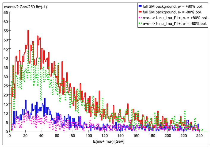
Figure 20: The muon energy distribution of the SM background after the smuon selection cuts described in the text have been imposed. The red(blue) solid curves correspond to the full background sample with $80\%$ LH(RH) electron beam polarization, and the green(pink) dotted lines represent the contribution from the process $e^{+}e^{-}\rightarrow l^{-}\bar{\nu}_{l}\nu_{l^{\prime}}{l^{\prime}}^{+},\,l=\mu,\tau$, with LH(RH) beam polarization, respectively. 250 fb^-1 of integrated luminosity for each beam polarization has been assumed.

As in the case of selectron production, there are only 22 out of 242 models which have kinematically accessible smuons at $\sqrt{s}=500$ GeV. The $\tilde{\mu}_{L(R)}$ is found to be kinematically accessible in 9(15) of these cases, there again being 2 models where both smuon states can be simultaneously produced. In the $\tilde{\mu}\to\mu\chi_{1}^{0}$ decay channel, smuons are observed by detecting a structure above the SM background in the muon energy distribution, similar to the search for selectrons. Here too, as is well-known, in the absence of such backgrounds, with high statistics and neglecting radiative effects, the 2-body decay of the $\tilde{\mu}$’s leads to horizontal shelf-like structures. In the more realistic situation where all such effects are included, the shelves remain but are now tilted downward (towards higher muon energies), as in the selectron case and have somewhat rounded edges. Examples of the muon energy spectra for some representative AKTW models displaying these effects are shown in Fig. 21 for either beam polarization configuration. Several things are to be noted in these Figures. The $\tilde{\mu}$ signals in the muon energy distribution vary over a wide range of both height and width depending upon the values of the $\tilde{\mu}$ and $\chi_{1}^{0}$ masses and the production cross sections. The range of possible signal shapes relative to the background is varied, but generally the signal is separable from the background in most models. We note again that the background is somewhat reduced compared to selectron production since there are fewer issues with beam remnants here. Again, we see that RH electron beam polarization leads to far smaller backgrounds than does LH beam polarization, as expected due to the diminished contribution from $W$-pair production.

Of the 22 kinematically accessible models, 19(17) lead to signals with significance $>5$ at these integrated luminosities with RH(LH) electron beam polarization. Combining the LH and RH polarization channels, we find that 19/22 models with accessible smuons lead to signals that meet our visibility criteria. We display a representative set of these models in Fig. 21 for both beam polarizations. The three models that do not pass our discovery criteria have smuons with masses in excess of 241 GeV; this leads to a strong kinematic suppression in their cross sections, and hence, very small signal rates. The $S/B$ ratio is somewhat small for some of the models in the LH polarization channel, as can be seen in Fig. 22, and are not so easily visible at this integrated luminosity. However, they nonetheless pass our significance tests for discovery.

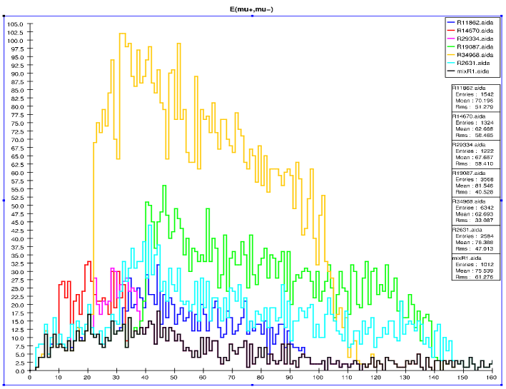
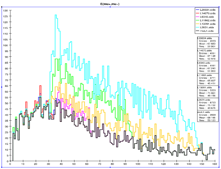
Figure 21: Muon energy distribution: the number of events/2 GeV bin (combined signal and background) after imposing the cuts described in the text for several representative models, with RH(LH) beam polarization in the top(bottom) panel, assuming an integrated luminosity of 250 fb^-1 for either polarization. The SM background is represented by the black histogram.

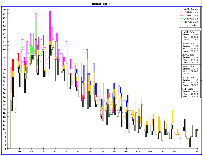
Figure 22: Same as the previous Figure but now showing AKTW models that result in a small $S/B$ ratio in the LH polarization channel in the $\tilde{\mu}$-pair analysis.

It is again interesting to compare the AKTW models that have visible smuons at the ILC with the well studied case of SPS1a’. Fig. 23 shows the muon energy spectrum we obtain after imposing our kinematic cuts in the case of SPS1a’ for both beam polarizations. As in our selectron analysis, we observe that the event yield for SPS1a’ is far larger than all the AKTW models we study here, in some cases by as much as a factor of order 50. Also, as in the previous analysis, two distinct shelves are observed since both $\tilde{\mu}_{L,R}$ are being simultaneously produced. The muon energy distribution is slightly different from that obtained for electrons in this model, not only because of the small differences in our cuts, but also due to the fact that the mixed final state $\tilde{\mu}_{L}\tilde{\mu}_{R}$ is not produced due to the absence of the $t$-channel contribution. Clearly, in comparison to the bulk of our models, it is rather trivial to discover and make precise determinations of the smuon properties in SPS1a’.

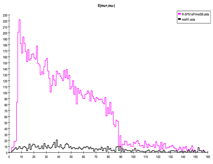
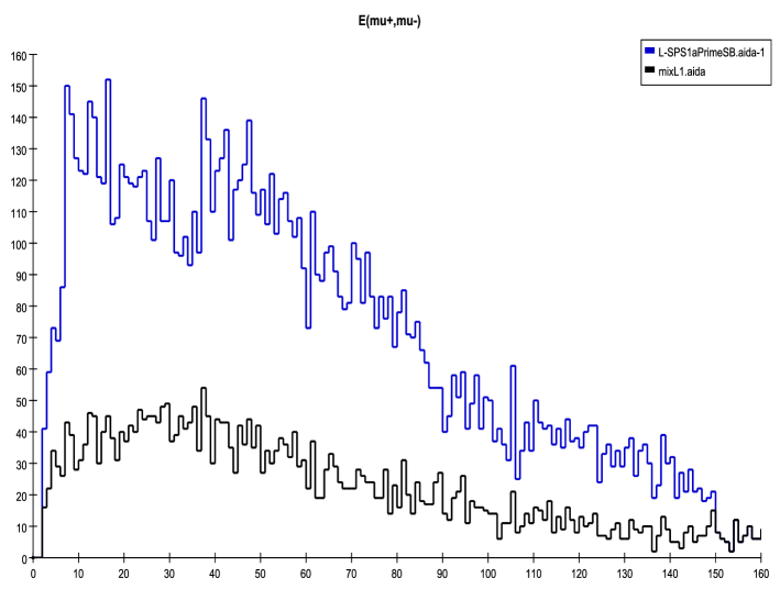
Figure 23: Muon energy distribution: the number of events/2 GeV bin (combined signal and background) after imposing the cuts described in the text for the benchmark model SPS1a’, with RH(LH) beam polarization in the top(bottom) panel, assuming an integrated luminosity of 250 fb^-1 for either polarization. The SM background is represented by the black histogram.

Note that 4 of the models with kinematically accessible smuons also have kinematically accessible lightest chargino states. However, since all of these charginos are rather close in mass to the LSP, i.e., within 5 GeV, the existence of the charginos does not constitute a large additional source of background and does not significantly affect the qualitative structure of the muon energy spectra. They could, however, modify the extracted values of the particle masses obtained from an analysis of the endpoints of the muon energy spectra and this possibility should be studied further.

Interestingly, as in the selectron case above, a number of models which do not have kinematically accessible smuons give rise to visible signals in the $\tilde{\mu}$-pair analysis. This is just another example of the well-known phenomenon where SUSY is a background to itself. We find that there are 20(15) models which yield fake signals in the case of RH(LH) polarization. As in the previous analysis, decays of other SUSY particles into muons, e.g., $\tilde{\chi}_{1}^{+}\to W^{*}\chi_{1}^{0}$ with $W^{*}\to\mu\nu$, can lead to the same observable final state in both polarization channels. We present examples of such misleading signals in Fig. 24. Note that in the case of RH beam polarization, the fake signature looks quite different than in a typical model which really has smuons present; there are no shelf-like structures and the muon energies are relatively low. This is to be expected when the final state muons are the result of a 3-(or more) body decay channel, and when chargino-neutralino mass splittings are small. However, for LH polarization, two representative fake models (labelled 8324 and 39331 in the Figures) appear to mimic the smuon shelf-like feature. This is due to the fact that in these particular models, as will be discussed further below in Section 5.1, the $W$ boson in the $\tilde{\chi}_{1}^{\pm}$ decay process is on-shell so that the final state muons are the result of true 2-body decays.

Figure 24: Muon energy distribution: the number of events/2 GeV bin (combined signal and background) after imposing the cuts described in the text for representative models which lead to fake smuon signatures from chargino and neutralino decays. Here, we show RH(LH) beam polarization in the top(bottom) panel, assuming an integrated luminosity of 250 fb^-1 for either polarization. The SM background is represented by the black histogram.

In order to assist in the differentiation of models with real smuons from ones that do not, it is necessary to examine other kinematic distributions. Figures 25 and  26 show the $p_{T}^{vis}$ distributions for the real smuon and fake models, respectively. Here we see that the models with real smuons generally lead to harder muons in the final state than do the counterfeit cases; this holds to some extent in the fake models where the charginos decay to on-shell $W$ bosons.

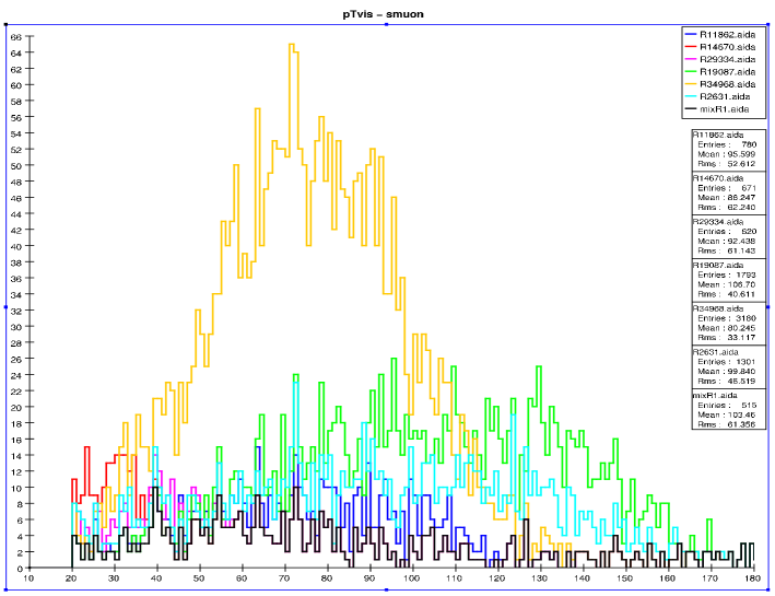
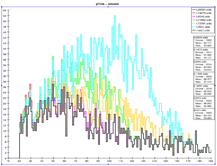
Figure 25: The $p_{T}^{vis}$ distribution for the same models shown in Fig. 21 with real smuons. Here, we show RH(LH) beam polarization in the top(bottom) panel, assuming an integrated luminosity of 250 fb^-1 for either polarization. The SM background is represented by the black histogram.

Figure 26: The $p_{T}^{vis}$ distribution for the same models shown in Fig. 24 with fake smuons. Here, we show RH(LH) beam polarization in the top(bottom) panel, assuming an integrated luminosity of 250 fb^-1 for either polarization. The SM background is represented by the black histogram.

IV.1.3 Staus

This analysis is similar to the other charged slepton analyses discussed above. We analyze the channel

$$\tilde{\tau}^{+}\tilde{\tau}^{-}\rightarrow\tau^{+}\tau^{-}\tilde{\chi}^{0}_{1}\tilde{\chi}^{0}_{1}\,,$$ (10)

that is, the signature is a tau pair plus missing energy. Staus are pair produced via $s$-channel $\gamma$ and $Z$ exchange and receive no $t$-channel contribution. The left- and right-handed staus mix to form two mass eigenstates, which have mixing-dependent couplings to the $Z$ boson. In contrast to the other charged slepton analyses above, the identification of the final state tau leptons is nontrivial, because the tau decays in the detector, predominantly into hadrons.

We focus on the hadronic decays of taus into pions, $\tau\rightarrow\pi\nu_{\tau};\,\tau\rightarrow\rho\nu_{\tau}\rightarrow\pi^{\pm}\pi^{0}\nu_{\tau};\,\tau\rightarrow 3\pi\nu_{\tau}$, the latter being a 3-prong jet, but also include the leptonic decays of the $\tau$. In the hadronic decay channel, taus are identified as jets with a charged multiplicity of 1 or 3, and with invariant mass less than some maximum value. Our tau selection criteria are as follows TimNorm ; Martyn:2004jc (note that we employ the notation tau-jet to describe the visible $\tau$ decay products):

1. We require 2 jets in the event, each with charged multiplicity of 1 (where the tau decays into a lepton, $\rho$, $\pi$, or $3\pi$-decay with $2\pi^{0}$s) or 3 (where the tau decays into 3 charged pions).

2. The invariant mass of tau-jet, i.e., the visible tau decay products, must be $<$ 1.8 GeV.

3. If the tau-jet is 3-prong (charged multiplicity of 3), then none of the charged particles should be an electron or muon.

4. If both tau-jets in the event are 1-prong, then we reject events where both jets are same flavor leptons, that is, an electron-positron or a muon pair. However we keep pairs of tau-jets that are, for example, an electron and a muon, or an electron and a pion, whereby a pion is defined as a charged track that is not identified as an electron or a muon.

As an alternative analysis, we follow the above criteria and allow leptonic tau decays into muons, but reject taus that decay into electrons. This reduces contamination from photon-induced backgrounds.

As mentioned above in our description of the SiD detector in Section III.2, the current detector design does not allow for tracking, and hence does not have the capability for particle ID, below $142$ mrad. Thus muons at low angles are completely missed if they are too energetic to deposit energy into clusters. As we will see, certain $\gamma$-induced processes constitute a significant background to stau production, particularly in the case where such energetic muons are produced but not reconstructed and the beam electron (or positron) receives a sufficient transverse kick to be detected. In this case, the final visible state is an electron and a muon, which would pass the standard tau ID preselection described above. The alternative tau preselection criteria, which rejects the electron decay channel, eliminates this background at the price of reducing the signal correspondingly by roughly 30%.

After these tau identification criteria are imposed, we employ cuts to reduce the SM background. Following Martyn:2004jc , we demand:

1. No electromagnetic energy (or clusters) in the region $|\cos\theta|>0.995$.

2. Two tau candidates as identified above, are weighted by their charge within the polar angle $-0.75<Q_{\tau}\cos\theta_{\tau}<0.75$. This reduces the $W$-pair background.

3. The acoplanarity angle must satisfy $\Delta\phi^{\tau\tau}>40$ degrees. Here, since we demand two tau candidates, the acoplanarity angle is equivalent to $\pi$ minus the angle between the $p_{T}$ of the taus, $\Delta\phi^{\tau\tau}=\pi-\theta_{T}$. The above requirement then translates to $\cos\theta_{T}>0.94$. This cut reduces the $W$-pair and $\gamma\gamma$-induced background.

4. $|\cos\theta_{p_{\mbox{\tiny}missing}}|<0.8$.

5. The transverse momentum of the ditau system be in the range $0.008\sqrt{s}<p_{T}^{\tau\tau}<0.05\sqrt{s}$. This decreases the $\gamma\gamma$-induced background.

6. The transverse momentum of each of the tau candidates be $p_{T}>0.001\sqrt{s}$. This cut is crucial to reduce the $\gamma\gamma$ and $e\gamma$ background.

7. The combined cut on $\sum p_{\perp,\vec{T}}^{\tau}$ and $\Delta\phi^{\tau\tau}$,

   $$\sum p_{\perp,\vec{T}}^{\tau} < 0.00125\sqrt{s}\left(1+5\,\sin\Delta\phi^{\tau\tau}\right)\,$$ (11)

   $$=0.00125\sqrt{s}\left(1+5\,\sqrt{1-\cos^{2}\theta_{T}^{\tau\tau}}\right)$$

   is imposed. Here, $\sum p_{\perp,\vec{T}}^{\tau}$ is the sum of the tau momenta projected onto the transverse thrust axis $\vec{T}_{\perp}$, where the transverse thrust axis is given by the $xy$-components of the thrust axis. This last cut is necessary in the tau decay channel to further decrease the $\gamma\gamma$ background.

As in the other slepton analyses, we histogram the resulting $\tau^{\pm}$ energy spectrum as well as $p_{T\mbox{\tiny vis}}$ in this case. We show the remaining SM backgrounds after these cuts are imposed in Fig. 27; the dominant background left after the cuts stems from $\gamma$-induced lepton-pair production processes.

In Fig. 27, we also display the effect of the alternative tau ID criteria discussed above. This alternative technique nearly completely eliminates the background since events where a beam electron/positron is falsely identified as a tau decay product are rejected. Of course, as mentioned above this technique also reduces the signal by approximately 30%. Augmenting the detector with muon ID capabilities at lower angles could reduce the $\gamma$-induced background without having to pay the price of introducing a restricted tau identification. As we will see below, a significant portion of the AKTW models have very low stau signal rates, and an improved tracking capability could be crucial if in fact this portion of the SUSY parameter space is realized in nature.

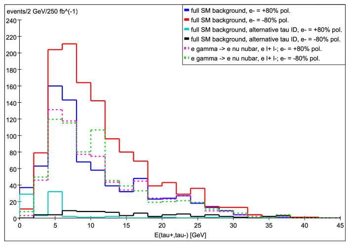
Figure 27: The $\tau^{\pm}$ energy spectrum of the SM background after the tau identification and stau selection cuts have been imposed. The solid blue and red lines are the full SM background for 80% right- (blue) and left-handed (red) electron polarization, the dashed lines (pink, right-handed, green left-handed) represent the dominant background source, $e^{\pm}\gamma\rightarrow e^{\pm}\nu\bar{\nu},e^{\pm}l^{+}l^{-},\,l=e,\mu,\tau$. Furthermore, the effect of eliminating the misidentification of beam electrons as tau decay products via the alternative tau ID described in the text is represented by the solid cyan line (80% right-handed beam polarization) and solid black line (80% left-handed polarization).

In 28 of the 242 AKTW models, the lightest stau is kinematically accessible for pair production at the 500 GeV ILC, and in one of these models the heavier stau partner can also be produced. The signal for stau production is somewhat different than in the case for selectrons and smuons as the final state tau decays in the detector. In this case, we no longer have the distinctive shelf-like feature in the resulting energy spectrum of the reconstructed tau. The shape of these spectra is highly dependent on the mass difference between the stau and the LSP as shown in Fig. 28, which displays the pure signal in 3 models before our selection cuts have been imposed. Here we see that small mass differences result in a sharply peaked distribution at low tau energies, while a larger mass difference yields a flatter distribution, albeit at a lower event rate. In principle, the search strategy, and hence the set of selection cuts, could be tailored to maximize the signal to background ratio once the stau$-$LSP mass difference is known. However, until the stau is discovered a general search strategy, such as that presented here, that applies for all mass regions must be employed.

Figure 28: Tau energy distribution stemming from stau pair production before our set of kinematic cuts have been imposed in three AKTW models. The red, blue, magenta histograms correspond to a stau-$\tilde{\chi}_{1}^{0}$ mass difference of order 25, 100, and 0.5 GeV, respectively.

Of these 28 models, we find that 18 lead to signals which can be observed at the significance level ${\cal S}>5$. We also find that the heavier stau with $m_{\tilde{\tau}_{2}}=240$ GeV is not produced with large enough event rates to be visible above the SM background. In addition, in 3 of these 28 models the mass difference between the lightest stau and the LSP is small enough such that the stau decays outside the detector, and it can be observed in our stable charged particle search (described below in Section 5.3). Of the 18 detectable stau models, 9(10) are visible via our standard search criteria in the LH(RH) beam polarization configuration. The total (combining signal and background) $\tau^{\pm}$ energy distribution is shown for a representative set of these models for both beam polarizations in Fig. 29. Here, we see that some of these models cleanly rise above the SM background, while others are just barely visible. The number of detectable stau signals is greatly increased when we apply our alternative set of preselection criteria discussed above. One finds that 17(12) models are observable with LH(RH) electron beam polarization; the tau energy spectrum for a sampling of these models is displayed in Fig. 30. In this case, we see that the signal is cleanly visible above the background for all models.

In all of the 18 models with observable staus, we find that the number of stau events that pass our cuts is dramatically reduced compared to the event rate in Fig. 28 before the cuts were applied. In addition, due to our cuts, the tau energy distribution is always peaked at low values, regardless of the stau-LSP mass difference, which ranges from $7-94$ GeV in these 18 models. In the 7 models where the signal is not observable, 2 are phase-space suppressed with $m_{\tilde{\tau}_{1}}>240$ GeV. The remaining 5 models all have reasonable $\tilde{\tau}_{1}$ masses and the $\tilde{\tau}_{1}-\tilde{\chi}_{1}^{0}$ mass difference ranges from $42-108$ GeV, but nonetheless have a small production cross section due to stau mixing.

Figure 29: Tau energy distribution: the number of events/2 GeV bin after imposing the standard set of tau ID and $\tilde{\tau}$ selection criteria described in the text for several representative AKTW models (signal and background combined). RH(LH) beam polarization is employed in the top(bottom) panel, assuming an integrated luminosity of 250 fb^-1 for each polarization configuration. The SM background corresponds to the black histogram.

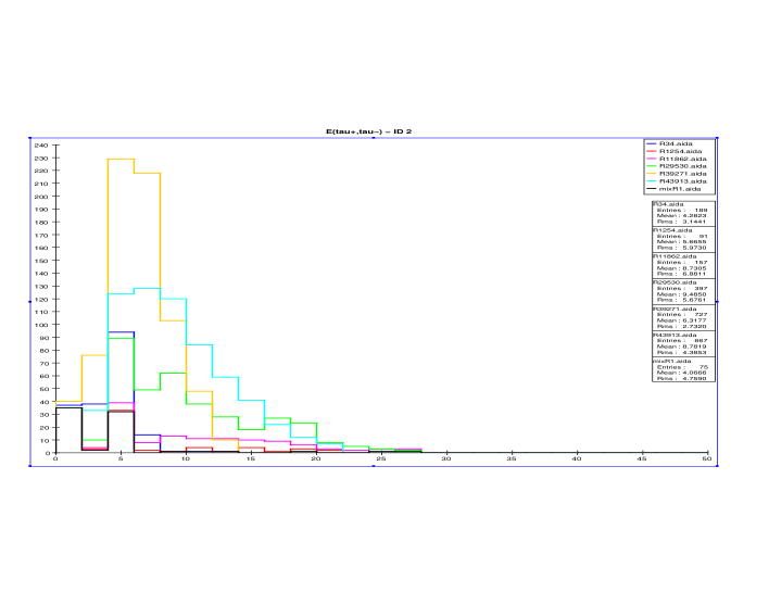
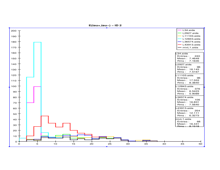
Figure 30: Tau energy distribution: the number of events/2 GeV bin after imposing the alternative set of tau ID and $\tilde{\tau}$ selection criteria described in the text for several representative AKTW models (signal and background combined). RH(LH) beam polarization is employed in the top(bottom) panel, assuming an integrated luminosity of 250 fb^-1 for each polarization configuration. The SM background corresponds to the black histogram.

Unlike many of the AKTW models we are examining, stau production at the ILC is straightforwardly observable in the case of the benchmark model SPS1a’. This holds in either of the analysis channels as can be observed in Figs. 31 and  32. Here we see that the stau signal is quite substantial and can be cleanly observed over the SM background for both choices of the electron beam polarization.

Figure 31: Same as in Fig. 29 except now for SPS1a’.

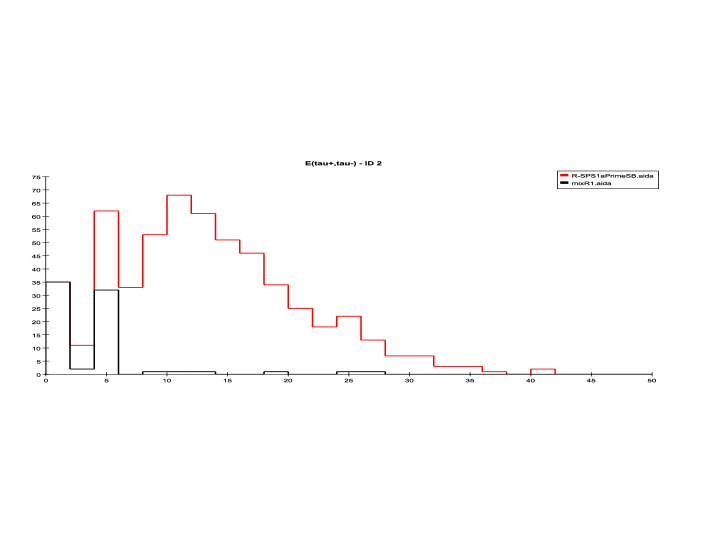
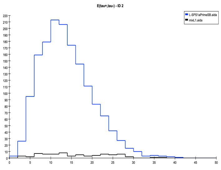
Figure 32: Same as in Fig. 30 except now for SPS1a’.

We find that many AKTW models which do not contain kinematically accessible stau states nonetheless give rise to visible signatures with significance $>5$ in this analysis, providing yet another example of SUSY being a background to itself. The tau energy distribution for a representative sampling of these SUSY background models is presented in Fig. 33, using the alternative set of kinematic cuts. We find that there are 29(28) models which yield fake signals with LH(RH) electron beam polarization in our standard set of kinematic cuts. For our alternative analysis which rejects electrons in the final state, there are 30(28) models with false signatures for the LH(RH) polarization configuration. This analysis clearly has a very large number of false signals. We note that in every one of these ”fake” models, $\tilde{\chi}_{1}^{\pm}\tilde{\chi}_{1}^{\mp},\,\tilde{\chi}_{2}^{0}\tilde{\chi}_{1}^{0}$, and $\tilde{\chi}_{2}^{0}\tilde{\chi}_{2}^{0}$ production is kinematically possible, and in one case selectron and smuon production is also viable. There are thus several sources of SUSY background which can lead to the same final state as that for stau pair production.

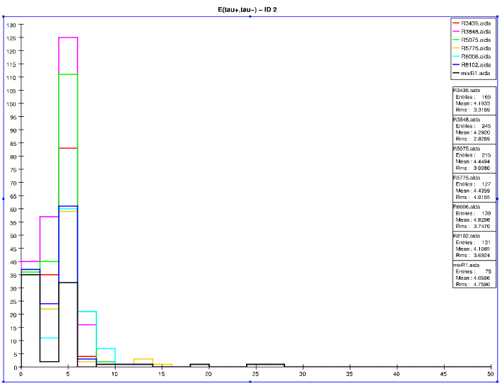
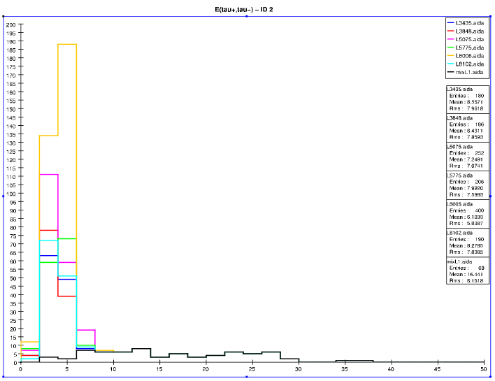
Figure 33: Tau energy distribution: the number of events/2 GeV bin after imposing the alternative set of tau ID and $\tilde{\tau}$ selection criteria described in the text for several representative AKTW models that give a fake signal in this channel. RH(LH) beam polarization is employed in the top(bottom) panel, assuming an integrated luminosity of 250 fb^-1 for each polarization configuration. The SM background corresponds to the black histogram.

In order to distinguish between stau production and these SUSY background sources, we investigate the variable

$$M_{\mbox{eff}}=E_{T}^{\mbox{miss}}+\sum_{i=1,2}|E_{T}^{\tau_{i}}|\,.$$ (12)

This variable is presented in Fig. 34 for both real and fake stau production. Here, we see that the false signals are slightly more peaked at lower values of $M_{\mbox{eff}}$ than does actual stau production. However, the distinction is not as clear as in the identification of selectron and smuon fake signatures discussed above, which makes use of the observable $p_{T}^{vis}$. This is because the full $\tau$ energy is not carried by its visible decay products. We note that the $p_{T}^{vis}$ observable is not effective in distinguishing stau states from SUSY background sources, as in this case both the staus and the background sparticles have multi-body decays.

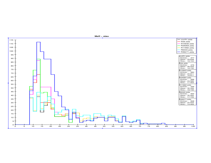
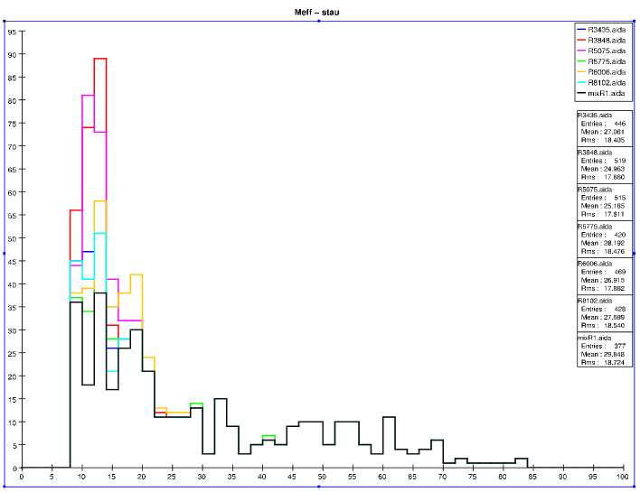
Figure 34: Effective mass (as employed at the LHC) of the products from the decays of objects identified as tau pairs produced from stau production (top panel) and from other, non-stau SUSY sparticles (bottom panel). Here we present the number of events/2 GeV bin assuming RH polarization and 500 fb^-1 of integrated luminosity for several models shown in comparison to the SM background represented as the black histogram.

IV.2 Sneutrino Pair Production

We now examine the neutral slepton sector, i.e., sneutrinos, which provides another potential handle for distinguishing between models. For all three sneutrino families there is the usual $Z$ boson exchange contribution to the production amplitude in the $s$-channel, while for electron sneutrinos there is an additional $t$-channel graph due to $\tilde{\chi}_{1,2}^{\pm}$ exchange. If the charginos are heavy, then the $Z$-exchange graph dominates for all three generations and the resulting production cross section is determined solely by the amount of available phase space. 11/242 of our AKTW models have electron or muon sneutrino pairs which are kinematically accessible at $\sqrt{s}=500$ GeV, while 18/242 models contain accessible tau sneutrinos. In one of the models the sneutrino is the LSP.

Sneutrinos, being neutral and weakly-interacting, are essentially only visible through their decay modes, of which there are several possible channels to consider: ($i$) $\tilde{\nu}_{\ell}\to\nu_{\ell}\tilde{\chi}_{1}^{0}$ largely dominates in most cases, but leads to an invisible final state which, by itself, is clearly useless for either discovery or model comparison. ($ii$) $\tilde{\nu}_{\ell}\to W\tilde{\ell}$ is kinematically forbidden as an on-shell mode when $\ell=e,\mu$ in all of our AKTW models and thus the corresponding 3-body branching fraction mediated by off-shell $W$ bosons is very small. However, due to large $\tilde{\tau}$ mixing, this 2-body mode is allowed for 6 of our models in the case of $\ell=\tau$. When both the $W$ and $\tau$ decay hadronically, we can search for final states with multiple jets plus missing energy in this case. ($iii$) $\tilde{\nu}_{\ell}\to\nu_{\ell}\tilde{\chi}_{2}^{0}$ can also occur, with the subsequent decay $\tilde{\chi}_{2}^{0}\to\tilde{\chi}^{0}_{1}jj$ via a $Z$ or Higgs boson. This occurs in 1(3) models in our sample when $\ell=e/\mu(\tau)$. However, in this case the resulting jets are likely to be relatively soft, due to a smaller $\tilde{\chi}_{2}^{0}-\tilde{\chi}_{1}^{0}$ mass difference, making this mode difficult to observe above background. $(iv)$ $\tilde{\nu}_{\ell}\to\tilde{\chi}_{1}^{+}\ell^{-}$ is accessible in 1(6) of these models when $\ell=e/\mu(\tau)$, and leads to a final state of multiple jets plus two charged leptons plus missing energy. As before, it is probable that these jets will be soft due to a smaller mass splitting between the chargino and the LSP and will most likely be difficult to observe depending upon the details of the rest of the spectrum.

We first study the final state $jjjjl^{+}l^{-}$ + missing energy. This final state results from the decays

$$\tilde{\nu} \rightarrow W\tilde{l}\rightarrow jjl\tilde{\chi}^{0}_{1}\,,$$

$$\tilde{\nu} \rightarrow l\tilde{\chi}_{1}^{\pm}\rightarrow ljj\tilde{\chi}^{0}_{1}\,.$$ (13)

For our signal selection, we require:

1. Precisely one opposite sign lepton pair and two jet-pairs and no other charged particles in the event.

2. No particles/clusters below the angular region of 100 mrad.

3. Missing energy to be $>2\,m_{\tilde{\chi}^{0}_{1},\mbox{\tiny min}}$. We take $m_{\tilde{\chi}^{0}_{1},\mbox{\tiny min}}=46$ GeV, which is the current (weak, yet model-dependent) bound on the mass of the lightest neutralino Yao:2006px . This bound arises from the invisible decay width of the $Z$ boson and holds unless the $\tilde{\chi}_{1}^{0}$ is very fine-tuned to be a pure Bino state and thus has no couplings to the $Z$ herbie2 . However, in order to estimate the effect on the background if this bound is increased, we perform a second analysis with $m_{\tilde{\chi}^{0}_{1},\mbox{\tiny min}}=100$ GeV.

4. In order to eliminate background that originates from very soft leptons or jets, we demand $E_{\mbox{\tiny jet},l}>0.01\sqrt{s}$.

These cuts effectively remove most of the SM background as can be seen in Fig. 35, which displays the missing energy distribution for the background sample. Here, we see that at large values of missing energy, the dominant background remaining after the cuts arises from the process $\gamma\gamma\to c\bar{c},b\bar{b}$. Unfortunately, the sneutrino signal rates are also small. Fig. 36 presents the results of our analysis: none of the sneutrino models rise above the background, but several of the ‘fake’ models, where the signals arise from other SUSY particles, do appear. 4(3) fake models yield visible signals in the case of RH(LH) beam polarization. The counterfeit signals here are due to chargino and neutralino production and decay. We find that increasing the minimum LSP mass to 100 GeV does not improve these results.

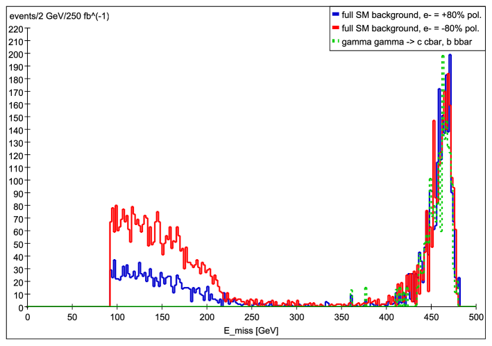
Figure 35: Missing energy distribution in 2 GeV bins for the SM background after the sneutrino selection cuts for the 4jet $+2\ell$ channel have been imposed. The blue(red) histogram corresponds to $80\%$ RH(LH) electron beam polarization. The green dotted curve corresponds to the dominant background source, $\gamma\gamma\to c\bar{c},b\bar{b}$. 250 fb^-1 of integrated luminosity was assumed for each polarization channel at 500 GeV.

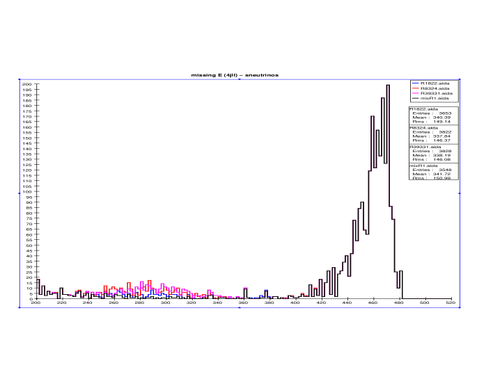
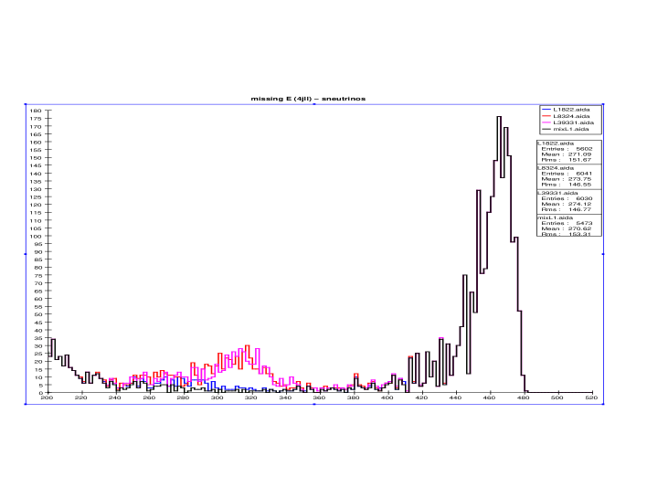
Figure 36: Missing energy distribution for the sneutrino $4j+$lepton pair analysis: the number of events/2 GeV bin for several the fake models, with RH(LH) beam polarization in the top(bottom) panel, assuming an integrated luminosity of 250 fb^-1 for either polarization. The SM background is shown as the black histogram.

We also study a second channel, with 6 jets and missing energy in the final state. This is produced from the decay $\tilde{\nu}\to W\tilde{\tau}\to jjj\tilde{\chi}^{0}_{1}$. The cuts and observables are similar to those of the $4j2\ell+$ missing energy analysis, with the obvious substitution that we demand precisely 6 jets and no other charged particles to appear in the event. We find that there is little to no SM background in this channel. However, we also find that none of our models are observable in this channel.

An additional possible way to observe sneutrinos is via the radiative process $e^{+}e^{-}\to\tilde{\nu}_{\ell}\tilde{\nu}_{\ell}+\gamma$. This may be particularly useful in the case where the decay channel $\tilde{\nu}_{\ell}\to\nu_{\ell}+\tilde{\chi}_{1}^{0}$ dominates. This reaction leads to a final state with a photon and missing energy and is thus similar to radiative LSP pair production, which we will discuss in detail below in Section 6.2. We find that radiative sneutrino production generally occurs with a smaller cross section than its LSP counterpart. As we will see below, the SM background from $e^{+}e^{-}\to\nu\bar{\nu}\gamma$ are generally too large to see this radiative process.

In the case of the SPS1a’ benchmark model, the sneutrino pair production mode is invisible as the sneutrinos dominantly decay into the $\nu\chi_{1}^{0}$ final state, as in most of our models here.

Taking these results together for these various sneutrino analyses, we conclude that the direct observation of $\tilde{\nu}_{\ell}$ production is very difficult, if not essentially hopeless for the set of AKTW models.

V Chargino Production

The chargino sector is simpler than that of the neutralinos as in the CP-conserving MSSM; it depends on only three real Lagrangian parameters at tree-level: $M_{2},\mu$, and $\tan\beta$. The resulting mass eigenstates, $\tilde{\chi}_{1,2}^{\pm}$, are thus general admixtures of the charged Wino and Higgsino weak states. Figure 37 displays the Wino/Higgsino content of the lightest chargino, $\tilde{\chi}_{1}^{\pm}$, in the 53 AKTW models that contain kinematically accessible charginos at $\sqrt{s}=500$ GeV. We see that the lightest chargino tends to be an almost pure Wino or Higgsino state in most of our models. In $e^{+}e^{-}$ collisions, such particles can be produced via two mechanisms; $s$-channel $\gamma,Z$ exchange produces either pure Wino or Higgsino pairs but no mixed Wino-Higgsino final states as the analogous $WZH^{\pm}$ coupling is absent. In addition, the $t-$channel sneutrino exchange amplitude produces pairs of charged winos only. Clearly, the cross section for chargino pair production not only depends on the eigenstate masses but also on the various mixing angles present in the chargino sector. At $\sqrt{s}=500$ GeV, $\tilde{\chi}_{2}^{\pm}$ pairs are typically too heavy to pair produce, so we will consider only $\tilde{\chi}_{1}^{\pm}$ pair production in our analysis below.

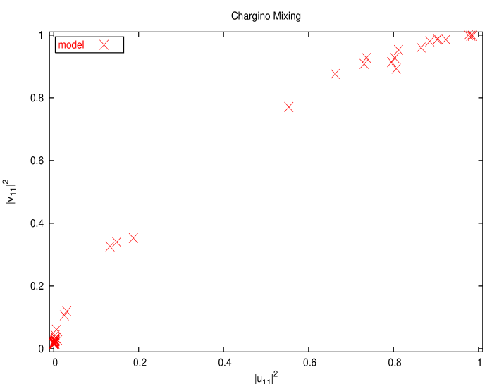
Figure 37: Wino/Higgsino content of the $\tilde{\chi}_{1}^{\pm}$ for the 53 models that have kinematically accessible charginos at $\sqrt{s}=500$ GeV. $U(V)$ is the left(right) diagonalizing matrix. In the lower left (upper right) corner of the Figure, the physical chargino is dominantly Higgsino (Wino).

Once produced, the detailed nature of the $\tilde{\chi}_{1}^{\pm}$ decays critically depends upon the mass difference $\Delta m_{\tilde{\chi}}=m_{\tilde{\chi}_{1}^{\pm}}-m_{\tilde{\chi}_{1}^{0}}$, with the latter being the LSP. In all cases, $\chi_{1}^{\pm}$ decay can proceed via either a $W$, $\tilde{\chi}_{1}^{\pm}\to W\tilde{\chi}_{1}^{0}$, or through an intermediate slepton, e.g., $\tilde{\chi}_{1}^{\pm}\to\ell\tilde{\nu},\tilde{\nu}\to\nu\tilde{\chi}_{1}^{0}$. As seen above in Fig. 4, and in Figs. 38 and  39, the mass spectrum of the models that have chargino states kinematically accessible at $\sqrt{s}=500$ GeV is such that the distribution of values for $\Delta m_{\tilde{\chi}}$ are concentrated in the region $<5$ GeV. The variation in $\Delta m_{\tilde{\chi}}$ yields several distinct signatures for $\tilde{\chi}_{1}^{\pm}$ production and thus all possible values of $\Delta m_{\tilde{\chi}}$ must be considered when performing our analysis. For example, if $\Delta m_{\tilde{\chi}}>M_{W}$ then on-shell $W$ bosons can be produced and may be identified either through their leptonic or hadronic decay modes. We thus consider channels such as $\tilde{\chi}_{1}^{\pm}\to jj\,E_{\mbox{\tiny miss}}$, with the dijets reconstructing to the $W$ mass, or $\tilde{\chi}_{1}^{\pm}\to\mu E_{\mbox{\tiny miss}}$, with the latter mode also covering decays through the slepton channels: $\tilde{\chi}_{1}^{\pm}\to\tilde{\mu}^{\pm}\nu,\mu^{\pm}\tilde{\nu}\to\mu E_{\mbox{\tiny miss}}$. Hence, in this region, we search for the final states $\tilde{\chi}_{1}^{+}\tilde{\chi}_{1}^{-}\to 4j\,E_{\mbox{\tiny miss}}$, $2j\,\mu^{\pm}\,E_{\mbox{\tiny miss}}$ or $\mu^{+}\mu^{-}\,E_{\mbox{\tiny miss}}$. For smaller values of $\Delta m$, but still greater than a few GeV, we search for the same final states although the dijets will no longer reconstruct to $M_{W}$. A more difficult region is reached when $\Delta m_{\tilde{\chi}}$ is only a few GeV or less, as then the visible part of the $\tilde{\chi}^{\pm}_{1}$ decays are very $\tau$-like. Fig. 4 shows this region of chargino-LSP mass splitting for the range $\Delta m_{\tilde{\chi}}<6$ GeV as a function of the chargino mass; we see that this region comprises the bulk of our models with accessible $\tilde{\chi}_{1}^{\pm}$ states at $\sqrt{s}=500$ GeV.

At the other end of the spectrum, we must consider the case of small values of $\Delta m_{\tilde{\chi}}\mathrel{\mathchoice{\lower 3.01385pt\vbox{\halign{$\matth\displaystyle\hfil#\hfil$\cr<\crcr\sim\crcr}}}{\lower 3.01385pt\vbox{\halign{$\matth\textstyle\hfil#\hfil$\cr<\crcr\sim\crcr}}}{\lower 3.01385pt\vbox{\halign{$\matth\scriptstyle\hfil#\hfil$\cr<\crcr\sim\crcr}}}{\lower 3.01385pt\vbox{\halign{$\matth\scriptscriptstyle\hfil#\hfil$\cr<\crcr\sim\crcr}}}}1$ GeV. The branching fractions for the $\tilde{\chi}_{1}^{\pm}$ decay channels in this case are presented in Fig. 40. If $\Delta m_{\tilde{\chi}}$ is very small, $\mathrel{\mathchoice{\lower 3.01385pt\vbox{\halign{$\matth\displaystyle\hfil#\hfil$\cr<\crcr\sim\crcr}}}{\lower 3.01385pt\vbox{\halign{$\matth\textstyle\hfil#\hfil$\cr<\crcr\sim\crcr}}}{\lower 3.01385pt\vbox{\halign{$\matth\scriptstyle\hfil#\hfil$\cr<\crcr\sim\crcr}}}{\lower 3.01385pt\vbox{\halign{$\matth\scriptscriptstyle\hfil#\hfil$\cr<\crcr\sim\crcr}}}}100$ MeV, then the chargino is long lived, and will travel many meters before decaying into an electron and missing energy. In such a case, we perform a massive stable charged particle search, determining the velocity of the $\tilde{\chi}_{1}^{\pm}$ via momentum and energy measurements. As $\Delta m_{\tilde{\chi}}$ increases from this tiny value and the thresholds for $\tilde{\chi}_{1}^{\pm}$ decay into the $\mu$ and pion(s) are passed, the chargino lifetime decreases substantially and the chargino now decays to soft charged particles. In this mass range there are two possible search techniques: one can either look for decays in the detector from (semi-)long-lived $\tilde{\chi}_{1}^{\pm}$ states, or tag these soft decays via photon emission off of the initial and final state particles. The latter corresponds to the radiative process $e^{+}e^{-}\to\tilde{\chi}_{1}^{+}\tilde{\chi}_{1}^{-}\gamma$ Gunion:2001fu ; Riles:1989hd , and is the approach we will pursue below.

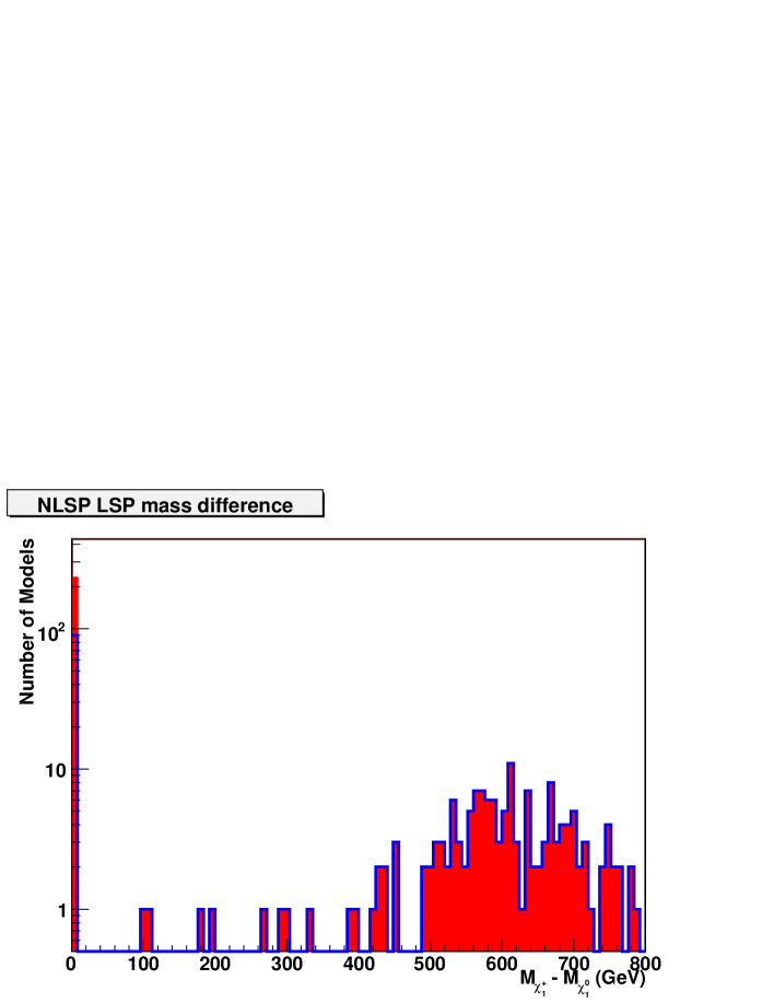
Figure 38: Lightest chargino-LSP mass difference for the region $0<\Delta m_{\tilde{\chi}}<800$ GeV. Note that the chargino states in the models where $\Delta m{\tilde{\chi}}>150$ GeV are not kinematically accessible at $sqrts=500$ GeV.

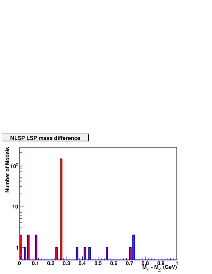
Figure 39: Lightest chargino-LSP mass difference for the close mass region $0<\Delta m_{\tilde{\chi}}<1$ GeV.

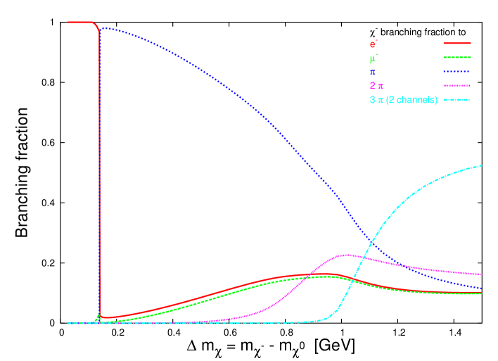
Figure 40: Branching fraction of $\tilde{\chi}_{1}^{\pm}$ as a function of $\Delta m_{\tilde{\chi}}$.

At $\sqrt{s}=500$ GeV, we find that 53/242 of the AKTW models have kinematically accessible charginos. Figure 38 shows that in all but two cases (which we label here as models 8324 and 39331) the models populate the region $\Delta m_{\tilde{\chi}}\leq 5.5$ GeV; for the two exceptions we see that $\Delta m_{\tilde{\chi}}>100$ GeV. Interestingly, we note that models with small $\Delta m\leq 1$ GeV tend to have a large Wino content, while those in the range $\Delta m_{\tilde{\chi}}\simeq 4\sim 5$ GeV are found to have a large Higgsino content as can be seen in Fig. 37.

We now discuss our analyses for each region of $\Delta m_{\tilde{\chi}}$.

V.1 Non-Close Mass Case

We first examine the case where

$$\Delta m_{\tilde{\chi}}\equiv m_{\tilde{\chi}^{\pm}}-m_{\tilde{\chi}^{0}_{1}}>1\mbox{ GeV}.$$ (14)

As already mentioned above, there are several possible final states that can be studied in this mass region. Analysis techniques have been developed for the cases where the chargino decay proceeds through on- or off-shell $W$ bosons (with $W\rightarrow jj$ or $W\rightarrow l\bar{\nu}_{l}$) or via sleptons (e.g., $\tilde{\mu}\rightarrow\mu\tilde{\chi}^{0}_{1}$). We discuss each of these in turn.

V.1.1 Chargino Decays via On-Shell $W$ bosons

This analysis applies to the case $\Delta m_{\tilde{\chi}}>M_{W}$. Here, we examine four-jet final states, stemming from the decays of the chargino pair into $W$ bosons with subsequent decays into quark pairs,

$$\tilde{\chi}_{1}^{+}\tilde{\chi}_{1}^{-}\rightarrow W^{+}W^{-}\tilde{\chi}^{0}_{1}\tilde{\chi}^{0}_{1}\,,$$ (15)

with

$$W^{\pm}\rightarrow q\bar{q}\,.$$ (16)

Taking the hadronic decay mode of both $W$ bosons yields the final state with the largest statistical sample.

As always, the SM background is significant. In order to reduce the background, we demand, as expanded and adapted from Williams ; Abbiendi:2003sc :

1. There be precisely 4 jets in the final state and no other charged particles. As mentioned in section III.2, we employ the JADE jet algorithm in the E scheme, with $y_{\mbox{\tiny cut}}=0.05$. This choice of $y_{cut}$ avoids the situation where soft gluons produce too many jets.

2. $E_{\mbox{\tiny vis}}>0$ in the backward direction. Here, the backward direction is defined with respect to the thrust axis, and corresponds to the hemisphere with the lesser amount of energy. This cut is designed to reduce SM background from $Z$ pair production, where one $Z$ boson decays into neutrinos, and the other $Z$ decays into quarks, which then radiate hard gluons.

3. In the forward direction, the visible energy is constrained to be $E_{\mbox{\tiny vis}}<\frac{1}{2}\sqrt{s}-m_{\tilde{\chi}^{0}_{1},\mbox{\tiny min}}$. As in the case of stau production, we take $m_{\tilde{\chi}^{0}_{1},\mbox{\tiny min}}=46$ GeV, which is the current bound on the mass of the lightest neutralino Yao:2006px in the case where the $\tilde{\chi}_{1}^{0}$ is not a pure Bino eigenstate.

4. The visible energy is constrained to be $E_{\mbox{\tiny vis}}<1$ GeV in the region $0.9\leq|\cos\theta|\leq 0.99$. This is to decrease the $W$ pair background which is strongly peaked in the forward direction.

5. The acoplanarity angle satisfy $\Delta\phi^{\mbox{\tiny jetpair}\,\mbox{ \tiny jetpair}}>30$ degrees. Since we demand that two jet pairs recombine into $W$ bosons, the acoplanarity angle is equivalent to $\pi$ minus the angle between the $p_{T}$ of the $W$ bosons, i.e., $\Delta\phi^{\mbox{\tiny jetpair}\,\mbox{\tiny jetpair}}=\pi-\theta_{T}$. This significantly reduces the $W$ pair and $\gamma\gamma$ background, since the $W$ bosons from the chargino decays are accompanied by missing energy from the LSP.

The standard search analysis for this final state is based on the energy distribution of the jet-pairs which reconstruct into a $W$ boson. As in the case of the selectron analysis, this distribution should have a box-like shape with a shelf and sharp endpoints in the presence of a high statistics, background-free, perfect detector environment with the absence of radiative effects. Here, the 2-body decay is taken to be $\tilde{\chi}_{1}^{\pm}\to W+\tilde{\chi}_{1}^{0}$ and the expressions in Eqs. (7)-(8) need to be adapted to include the massive $W$ boson. In this case, one can solve the equations for the chargino and LSP masses and finds

$$m_{\tilde{\chi}_{1}^{\pm}}^{2} = \frac{A\pm B}{2(E_{\max}+E_{\min})^{2}/s}\,,$$ (17)

$$m_{\tilde{\chi}^{0}_{1}}^{2} = m_{\tilde{\chi}_{1}^{\pm}}^{2}+m_{W}^{2}\left(1-2\frac{(E_{\max}+E_{\min})}{\sqrt{s}}\right)\,,$$ (18)

where

$$A=m_{W}^{2}+E_{\max}E_{\min},$$ (19)

$$B=\sqrt{(m_{W}^{2}-E_{\max}^{2})(m_{W}^{2}-E_{\min}^{2})},$$ (20)

and where $E_{\max}$, $E_{\min}$ are determined experimentally.

We refrain from presenting the remaining SM background after these cuts are imposed, as only a handful of events pass the cuts. As mentioned above, only 2 models in our sample lie in the kinematic region $\Delta m_{\tilde{\chi}}>M_{W}$. The jet-pair energy distribution for these two cases is displayed in Fig. 41 for left- and right-handed electron beam polarization. Here, we see that the overall event rate that survives the kinematic cuts is not large, but the signal cleanly towers above the even smaller background. We can see the effects of the cuts and the detector environment in these cases, as the shape of the spectrum does not display the shelf-like behavior discussed above. Note that an additional model (labelled 1822), which has $\Delta m_{\tilde{\chi}}\sim 1$ GeV, also passes the kinematic cuts for this analysis. This model yields a smaller event rate than the cases with on-shell $W$ bosons, but populates a different region of the spectrum. However, this model contains a light $\tilde{\chi}_{1,2}^{\pm}\,,\tilde{\chi}_{1,2,3}^{0}$ sector and the signal that passes our cuts here is due to the production of these heavier gaugino states and not from the $\tilde{\chi}_{1}^{+}$ and is thus a fake. Three out of 53 AKTW models with accessible charginos are thus visible with a significance ${\cal S}>5$ in this channel. We note that fake signals from the production of other SUSY particles do not satisfy our visibility criteria in this channel, except for model 1822. It would thus seem that this analysis is relatively free from Supersymmetric backgrounds, at least in the case of the AKTW models.

In summary, if $\Delta m_{\tilde{\chi}}$ is large enough to produce on-shell $W$ bosons, this is clearly a very clean channel.

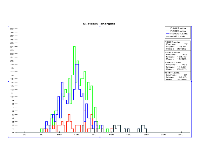
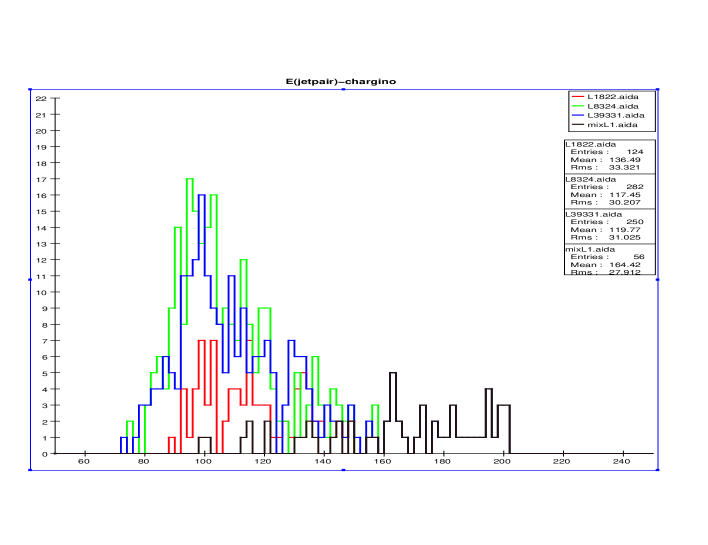
Figure 41: Jet-pair energy distribution: the number of events/2 GeV bin after imposing the full set of cuts discussed in the text for chargino production and on-shell decays to a $W$ boson for the three models which are visible in this channel. RH(LH) beam polarization is employed in the top(bottom) panel, assuming an integrated luminosity of 250 fb^-1 for either polarization. The SM background is shown as the black histogram.

V.1.2 Chargino Decays via Off-Shell $W$s and/or Sleptons

We search for three final states in the kinematic region $M_{W}>\Delta m_{\tilde{\chi}}>1$ GeV where the $W$ boson is produced off-shell in the $\tilde{\chi}_{1}^{\pm}$ decay: four jet events plus missing energy, two jets and a lepton plus missing energy or two leptons plus missing energy. In order to avoid the large SM background from the beam remnants in $\gamma e^{\pm}$, $\gamma\gamma$ reactions, we require that the final state leptons be muons.

In the fully leptonic decay channel, the kinematic cuts we employ barron to distinguish signal from background are very similar to the slepton searches described in Section IV above. As in the case of smuon production, one searches for a structure above the SM background in the final state muon energy distribution. Here, however, the signal distribution is not expected to display the by-now familiar shelf-like behavior, due to the 3-body nature of the chargino decay. Examples of the muon energy spectra for some representative AKTW models are shown in Fig. 42 for both beam polarization states. Here, we see that the $E_{\mu}$ spectrum for the signal varies greatly in size and shape between the various models depending on the value of $\Delta m_{\tilde{\chi}}$ and the production cross section, but is nonetheless clearly separable from the SM background for these cases. Comparing with Fig. 21 we note that the SM background has a similar shape, but is slightly larger throughout the spectrum in this analysis. As usual, RH electron beam polarization leads to a smaller SM background since the $t$-channel contribution to $W$ pair production is suppressed in this case.

Of the 53 models with kinematically accessible $\tilde{\chi}_{1}^{\pm}$ states, we find that 12(11) lead to visible signals over the background at a significance of ${\cal S}>5$ for RH(LH) electron beam polarization. Combining the two polarization channels, a total of 14/53 models meet our visibility criteria. From Fig. 42 we note, however, that $S/B$ can be small enough in some cases to render a detailed study of the chargino properties difficult.

SUSY can be a substantial background to itself in this channel, with smuon production being a particularly large background source. We find that 14(12) models yield fake signals that pass our visibility criteria for a RH(LH) polarization configuration. We note that in all cases, the counterfeit signal indeed arises from the production of smuons. The muon energy distribution for some representative examples of such misleading signals are presented in Fig. 43. From the Figure, we see that the signal tends to have a shelf-like behavior, as would be expected for smuon production, and thus looks quite different than the case of chargino production.

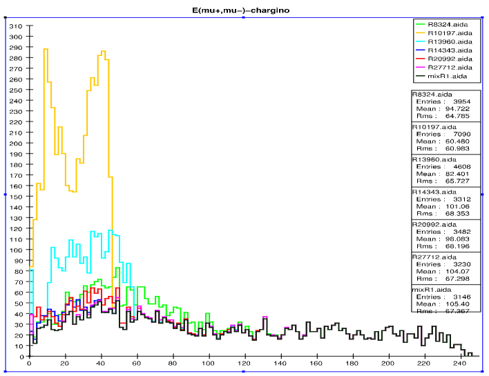
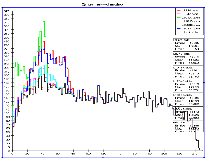
Figure 42: Muon energy distribution: the number of events/2 GeV bin after imposing the full set of cuts discussed in the text for chargino production for representative models which are visible in this channel. RH(LH) beam polarization is employed in the top(bottom) panel, assuming an integrated luminosity of 250 fb^-1 for either polarization. The SM background is shown as the black histogram.

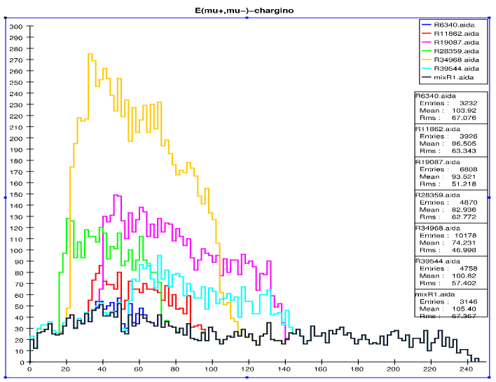
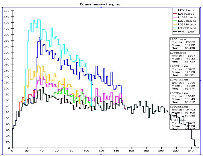
Figure 43: Muon energy distribution: the number of events/2 GeV bin after imposing the full set of cuts discussed in the text for representative models which fake a chargino signal in this channel. RH(LH) beam polarization is employed in the top(bottom) panel, assuming an integrated luminosity of 250 fb^-1 for either polarization. The SM background is shown as the black histogram.

We now turn to the fully hadronic channel, where the final state is 4 jets plus missing energy. We employ the following kinematic cuts (based on, e.g., Abbiendi:2003sc ):

1. There be precisely 4 jets in the final state and no other charged particles.

2. No tracks (or clusters) be present below an angle of 100 mrad. This reduces photon-initiated backgrounds.

3. Missing energy is constrained to be $>0.5\sqrt{s}$. This favors the signal, which contains a large amount of missing energy compared to many background sources.

4. In the forward direction, the visible energy is constrained to be $E_{\mbox{\tiny vis}}<\frac{1}{2}\sqrt{s}-m_{\tilde{\chi}^{0}_{1},\mbox{\tiny min}}$. We, again, take $m_{\tilde{\chi}^{0}_{1},\mbox{\tiny min}}=46$ GeV. However, in order to estimate the effect on the background if this bound is increased, for example by future studies at the LHC, we perform a second analysis with $m_{\tilde{\chi}^{0}_{1},\mbox{\tiny min}}=100$ GeV.

5. We require precisely two jets in each hemisphere as determined by the thrust axis. This cut eliminates jets stemming from $\tau$ decays arising from tau pair production, where one $\tau$ has a one-prong decay, and the other is 3-prong.

6. We reconstruct the off-shell $W$ bosons by coalescing the 4 jets into 2, one for each $W$ boson. We force this by adjusting the $y_{\mbox{\tiny cut}}$ parameter of the JADE jet finding algorithm until two jets are found (see Section III for details of the algorithm), and then require the resulting dijet invariant masses to be $>2$ GeV.

The first observable we consider for this channel is the missing energy distribution, where we expect a peak from the signal at large values of $E_{\rm miss}$. This spectrum is presented in Fig. 44 where the black histogram corresponds to the SM background, as usual. We find that a particularly troublesome background arises from the process $\gamma\gamma\rightarrow q\bar{q}$. It is clear from the Figure that this background reaction stubbornly yields a significant event rate even after the above cuts are imposed. The missing energy spectra for representative AKTW models are also shown in the Figure for both polarization states and by eye seem barely visible above the background. However, the statistical sample is large, and nonetheless, chargino production in several AKTW models are observable in this channel. We find that 9(31) models are observable with significance $>5$ in the RH(LH) polarization state. All models that are visible with RH beam polarization are also observed with LH beam polarization. If we increase the minimal value of the bound on the LSP mass to 100 GeV as mentioned in the kinematic cuts above, we find that 4 additional models satisfy our visibility criteria. We note that the production of other Supersymmetric particles do not pass our cuts in this channel and hence there are no ‘fake’ signals.

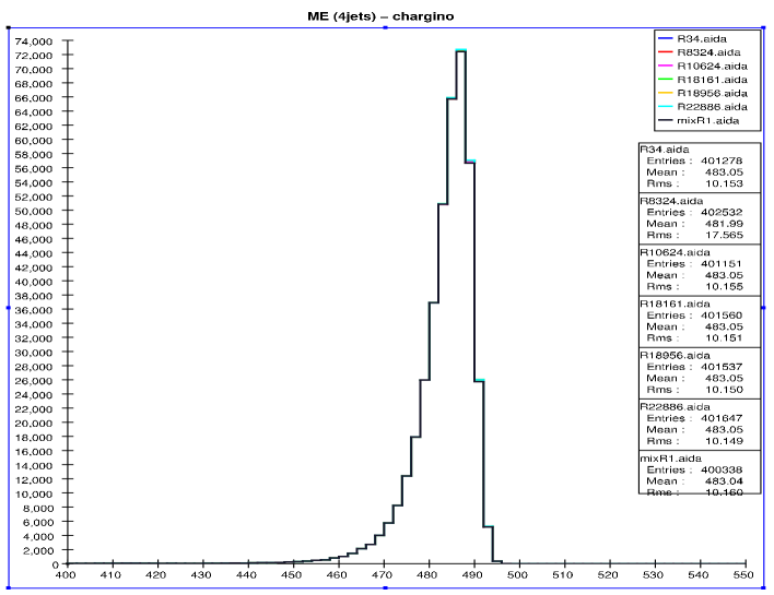
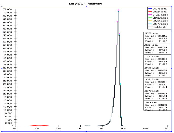
Figure 44: Missing energy distribution: the number of events/2 GeV bin after imposing the full set of cuts discussed in the text for the fully hadronic chargino decay channel for representative models which are visible in this channel. RH(LH) beam polarization is employed in the top(bottom) panel, assuming an integrated luminosity of 250 fb^-1 for either polarization. The SM background is shown as the black histogram.

We next examine the distribution of the two dijet invariant masses to see if the photon-induced background is less problematic for this observable. Figure 45 displays the SM background for this case for both electron beam polarizations. Here, we see that the background from two-photon initiated processes is still significant, with the dominant channel passing the cuts being $\gamma\gamma\to q\bar{q}$. The results for the AKTW models are presented in Fig. 46 for both electron beam polarizations. We find that with RH polarization none of the AKTW models with chargino decays into off-shell $W$ bosons are visible over the background in this observable. In the case of LH electron beam polarization, we find that 2 such models (labelled as 12843 and 14343) are detectable with a significance $>5$. These models yield an excess of events in the first two bins of the distribution; this excess is not visible by eye, but is statistically significant due to the large sample size. The two models with chargino decays into on-shell $W$ bosons (labelled as 8324 and 39331) display a clear signal for both beam polarizations as shown in the Figure. We see that the invariant $M_{jj}$ spectrum is broader for these two models and yields a high event rate at large invariant masses. If the minimum value of the LSP mass is raised to 100 GeV in our kinematic cuts, we find that only the on-shell $W$ boson decays are visible above the background. One additional model (labelled as 1822) is also distinguishable from the background. In this case, however, it is due to the pair production of $\tilde{\chi}_{2}^{0}$ states, with their subsequent decays into $Z+\tilde{\chi}_{1}^{0}\to 2{\rm jets}+\tilde{\chi}_{1}^{0}$, that passes our cuts and provides a fake signal.

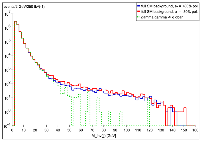
Figure 45: Distribution of dijet invariant masses from the remaining SM background after the chargino 4-jet selection cuts listed in the text have been imposed. This is generated for $250\mbox{ fb}^{-1}$ of SM events with 80% right-handed (solid blue line) and 80% left-handed (solid red line) electron beam polarization, and unpolarized positron beam at $\sqrt{s}=500$ GeV. The dashed green line shows the main processes contributing to the background, $\gamma\gamma\rightarrow q\bar{q}$, which is independent of the beam polarization.

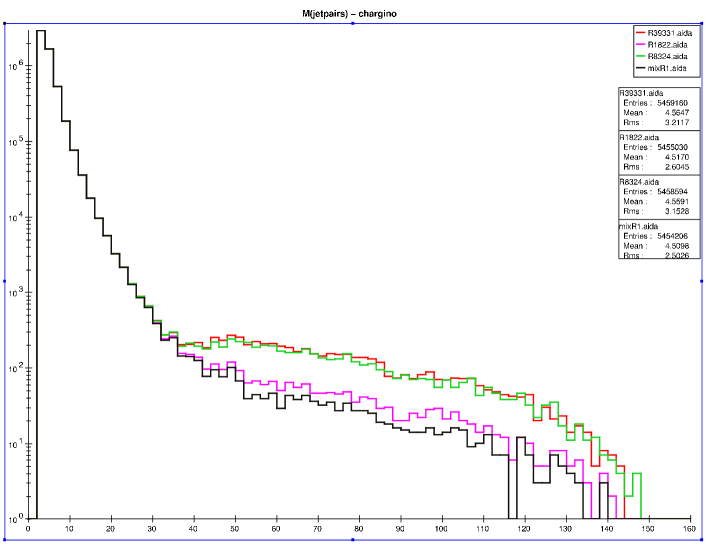
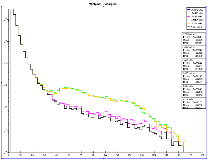
Figure 46: Jet-pair invariant mass distribution: the number of events/2 GeV bin after imposing the full set of cuts discussed in the text for the fully hadronic decays of the chargino for representative models which are visible in this channel. RH(LH) beam polarization is employed in the top(bottom) panel, assuming an integrated luminosity of 250 fb^-1 for either polarization. The SM background is shown as the black histogram.

Further attempts to decrease the SM background in the 4-jet channel prove to be difficult and tend to remove the signal as well as the background. This is because the characteristics of the signal and remaining background are similar for variables such as the missing energy spectrum, acoplanarity, and $p_{T\mbox{\tiny vis}}$ (see Fig. 47). In particular, both signal and background distributions peak at low values of $p_{T\mbox{\tiny vis}}$ and acoplanarity and at high values of missing energy as discussed above. Previous searches for charginos in the literature (e.g., Abbiendi:2003sc ) have employed additional cuts on $p_{T\mbox{\tiny vis}}$ and/or acoplanarity. In particular, we find that an additional restriction on the transverse momentum,

1. $p_{T\mbox{\tiny vis}}>0.06\sqrt{s}$

effectively reduces the background as shown in Fig. 48, but also removes the signal for all of the AKTW models with chargino decays into off-shell $W$ bosons. We show the effect of this additional cut on transverse momentum in the missing energy and jetpair invariant mass distributions in Figs. 49 and 50 for both electron beam polarizations. Here, we display all of the AKTW models which yield a visible signal with significance $>5$. We see that the signal for the models where the chargino decays into on-shell $W$ bosons (labelled as 8324 and 39331) towers above the background for both observables with both beam polarizations. As we saw above, the visible signal for model 1822 is due to the production of $\tilde{\chi}_{2}^{0}$ states and is thus fake. We emphasize that none of the AKTW models with chargino decays into off-shell $W$ bosons are observable once this additional $p_{T}$ cut is applied.

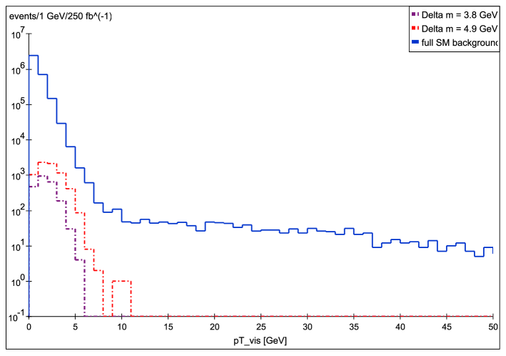
Figure 47: Transverse momentum distribution of remaining SM background after the chargino 4-jet selection cuts listed in the text have been imposed. This is generated from $250\mbox{ fb}^{-1}$ of SM events with 80% left-handed electron beam polarization, and unpolarized positron beam at $\sqrt{s}=500$ GeV (solid blue line). The dashed purple and red lines show signal events produced in two AKTW models that are representative for the class of models with $\Delta m_{\tilde{\chi}}$ of the order of a few GeV.

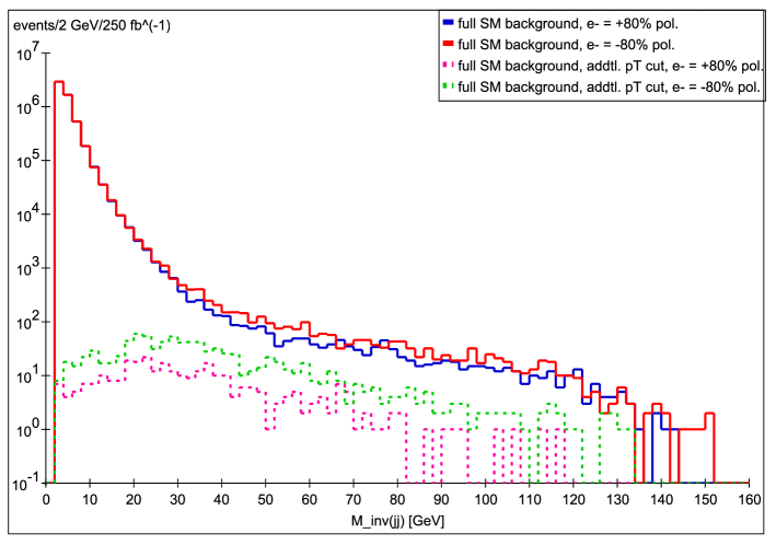
Figure 48: Distribution of dijet invariant masses from the remaining SM background after the chargino 4-jet selection cuts listed in the text have been imposed with the additional cut on transverse momentum. This is generated from $250\mbox{ fb}^{-1}$ of SM events with 80% right-handed (dashed pink line) and 80% left-handed (dashed green line) electron beam polarization, and unpolarized positron beam at $\sqrt{s}=500$ GeV. The solid lines are as in fig. 45.

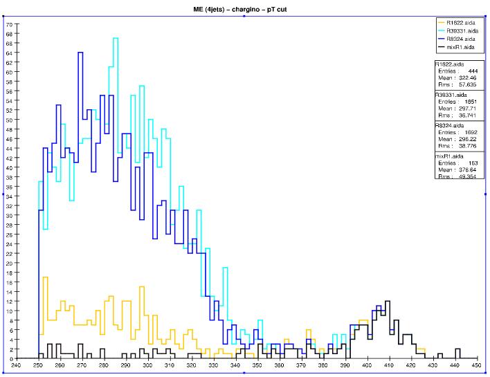
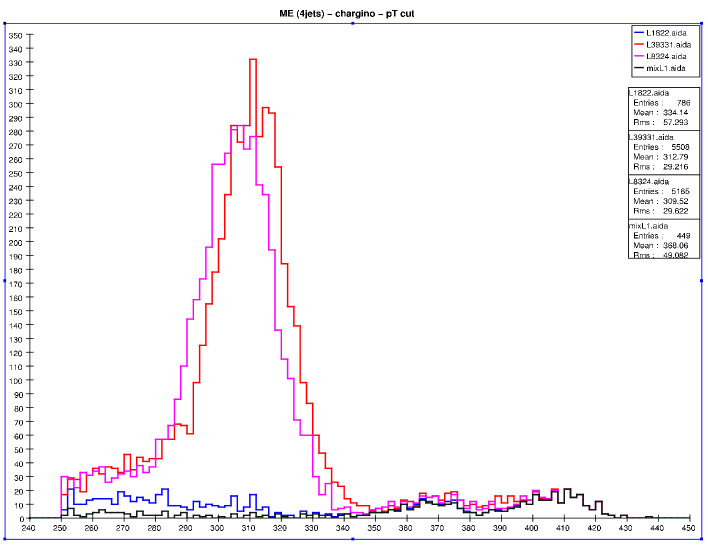
Figure 49: Missing energy distribution: the number of events/2 GeV bin after imposing the full set of cuts discussed in the text for the fully hadronic chargino decay channel, including an additional cut on transverse momentum, for representative models which are visible in this channel. RH(LH) beam polarization is employed in the top(bottom) panel, assuming an integrated luminosity of 250 fb^-1 for either polarization. The SM background is shown as the black histogram.

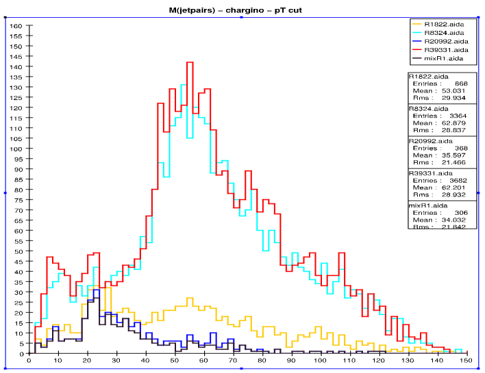
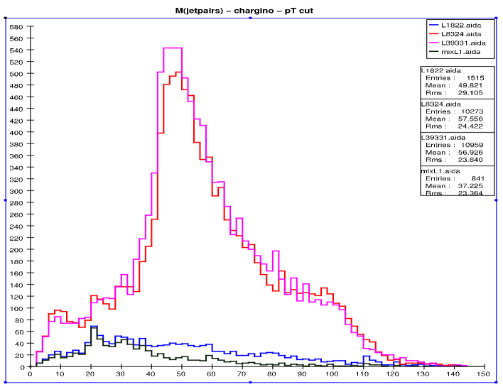
Figure 50: Jet-pair invariant mass distribution: the number of events/2 GeV bin after imposing the full set of cuts discussed in the text for the fully hadronic chargino decay channel, including an additional cut on transverse momentum, for representative models which are visible in this channel. RH(LH) beam polarization is employed in the top(bottom) panel, assuming an integrated luminosity of 250 fb^-1 for either polarization. The SM background is shown as the black histogram.

Lastly, we examine the mixed decay channel,

$$\tilde{\chi}_{1}^{+}\tilde{\chi}_{1}^{-}\rightarrow q\bar{q}\tilde{\chi}_{1}^{0}+\mu\bar{\nu}_{\mu}\tilde{\chi}_{1}^{0}\,,$$ (21)

which can proceed via (if kinematics allow)

$$\tilde{\chi}_{1}^{+}\tilde{\chi}_{1}^{-}\to W^{*\,\pm}\tilde{\chi}^{0}_{1}+\mu^{\mp}\tilde{\nu}_{\mu},W^{*\,\pm}\tilde{\chi}^{0}_{1}+\tilde{\mu}^{\mp}\nu_{\mu}$$ (22)

with

$$W^{*\,\pm}\rightarrow q\bar{q}\,,$$ (23)

or via

$$\tilde{\chi}_{1}^{+}\tilde{\chi}_{1}^{-}\rightarrow W^{*\,+}W^{*\,-}\,,$$ (24)

where one of the virtual $W$ bosons decays hadronically while the other decays leptonically into a muon.

For this channel, we employ the cuts

1. There be 2 jets (with no muonic component) plus one muon with no other visible particles in the final state.

2. There be no tracks or clusters of energy within 100 mrad of the beampipe as the signal is peaked at wide angles.

3. The visible energy satisfy $E_{\mbox{\tiny vis}}<\frac{1}{2}\sqrt{s}-m_{\tilde{\chi}^{0}_{1},\mbox{\tiny min}}$ in the forward direction. As above, we take $m_{\tilde{\chi}^{0}_{1},\mbox{\tiny min}}=46$ GeV Yao:2006px . However, in order to estimate the effect on the background if this bound is increased, we perform a second analysis with $m_{\tilde{\chi}^{0}_{1},\mbox{\tiny min}}=100$ GeV.

4. The invariant mass of the jet-pair be larger than 2.4 GeV. This cut is used to eliminate jets stemming from $\tau$ decays.

Here, we examine the energy and invariant mass of the jet-pair. We find that the same issues discussed above in the 4-jet channel regarding potential additional cuts based on acoplanarity and transverse momentum are also relevant in this case and thus these cuts are not employed in our analysis. The background remaining after our cuts are imposed is presented in Fig. 51 for the invariant mass distribution, where the dominant remaining SM background processes are $\gamma\gamma\rightarrow q\bar{q},\,\gamma\gamma\rightarrow\tau^{+}\tau^{-}$ and $e^{+}e^{-}\rightarrow q\bar{q}^{\prime}l\bar{\nu}_{l}$. We see that the background distribution is roughly the same for both beam polarizations as is to be expected for $\gamma\gamma$ induced processes.

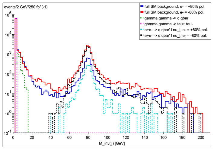
Figure 51: Distribution of dijet invariant mass from the remaining SM background after the chargino 2-jet plus muon selection cuts listed in the text have been imposed. This is generated from $250\mbox{ fb}^{-1}$ of SM events with 80% right-handed (solid blue line) and 80% left-handed (solid red line) electron beam polarization, and unpolarized positron beam at $\sqrt{s}=500$ GeV. The other dashed, and solid lines show the main processes contributing to the background, $\gamma\gamma\rightarrow q\bar{q}$ (dashed green line), $\gamma\gamma\rightarrow\tau^{+}\tau^{-}$ (dashed pink line), which are independent of beam polarization, and $e^{+}e^{-}\rightarrow q\bar{q}^{\prime}l\bar{\nu}_{l}$, for 80% right-handed (solid cyan line) and 80% left-handed (solid black line) electron polarization.

The invariant mass spectrum for the case where the charginos decay to off-shell $W$ bosons is displayed in Fig. 52 for both beam polarizations. In both cases, the signal rises above the background in the region of smaller ($<60$ GeV) invariant masses of the jet pair, as is expected due to the off-shell nature of the $W$ bosons. The model labelled as 1822 also shows a visible signature, with a peak located at $M_{jj}\sim 80-90$ GeV. As we saw above, this is due to $\tilde{\chi}_{2}^{0}$ production in this model with the subsequent decay $\tilde{\chi}_{2}^{0}\to Z+\tilde{\chi}_{1}^{0}$ with the $Z$ decaying hadronically and is a false signal. The $M_{jj}$ distribution for the 2 AKTW models where the charginos decay to on-shell $W$ bosons is shown in Fig. 53. Here, we would expect to see a peak above the SM background in the distribution around $M_{W}$, and indeed, that is the case. In summary, we find that 23(35) of the AKTW models with kinematically accessible charginos lead to signals in this observable with a visibility significance ${\cal S}>5$ for RH(LH) electron beam polarization at these integrated luminosities. We note that none of the AKTW models are visible over the background in the case where the minimum value of the LSP mass is increased to 100 GeV as described in our cuts.

The second observable we examine in this analysis is the energy of the jet pair which is displayed in Fig. 54 for several AKTW models where the chargino decays to an off-shell $W$ boson. Again, we see that the signal rises above the background for lower values of $E_{jj}$ ($\mathrel{\mathchoice{\lower 3.01385pt\vbox{\halign{$\matth\displaystyle\hfil#\hfil$\cr<\crcr\sim\crcr}}}{\lower 3.01385pt\vbox{\halign{$\matth\textstyle\hfil#\hfil$\cr<\crcr\sim\crcr}}}{\lower 3.01385pt\vbox{\halign{$\matth\scriptstyle\hfil#\hfil$\cr<\crcr\sim\crcr}}}{\lower 3.01385pt\vbox{\halign{$\matth\scriptscriptstyle\hfil#\hfil$\cr<\crcr\sim\crcr}}}}M_{W}$), except for the case of model 1822 which is a fake as described above. For comparison, the results for the two models which have decays to on-shell $W$ bosons are shown in Fig. 55, where we see that the $M_{jj}$ spectrum is peaked at larger values in this case. For this observable, we find that 26(35) of the AKTW models meet our visibility criterion. We note that two more models are visible with RH polarization in this observable compared to the $M_{jj}$ distribution discussed above. Again, none of the models are visible when the minimum value of the LSP mass is increased in the analysis.

Except for model 1822, we note that there are no fake signals from the production of other SUSY particles for either observable in this channel.

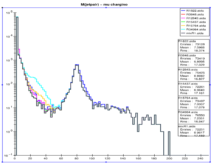
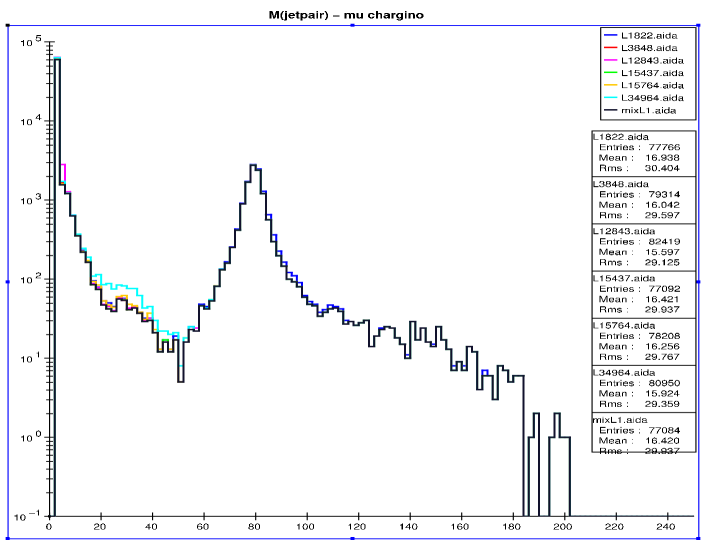
Figure 52: Jet-pair invariant mass distribution: the number of events/2 GeV bin after imposing the full set of cuts discussed in the text for the 2-jet $+\mu$ channel with $\Delta m_{\tilde{\chi}}<M_{W}$ for representative models which are visible in this channel. RH(LH) beam polarization is employed in the top(bottom) panel, assuming an integrated luminosity of 250 fb^-1 for either polarization. The SM background is shown as the black histogram.

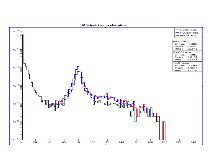
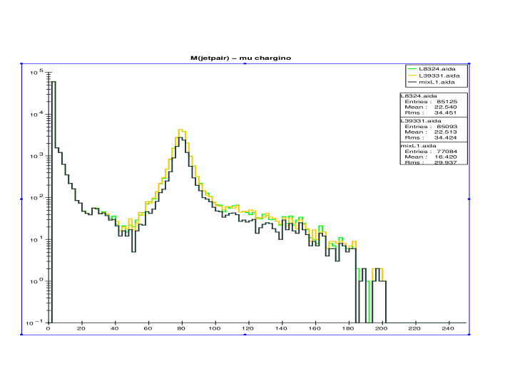
Figure 53: Jet-pair invariant mass distribution: the number of events/2 GeV bin after imposing the full set of cuts discussed in the text for the 2-jet $+\mu$ channel with $\Delta m_{\tilde{\chi}}>M_{W}$ for representative models which are visible in this channel. RH(LH) beam polarization is employed in the top(bottom) panel, assuming an integrated luminosity of 250 fb^-1 for either polarization. The SM background is shown as the black histogram.

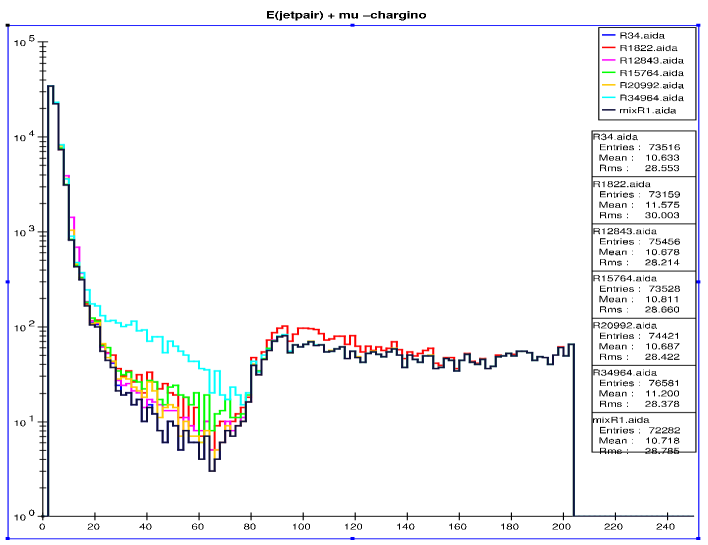
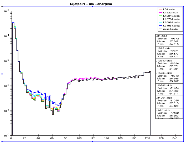
Figure 54: Jet-pair energy distribution: the number of events/2 GeV bin after imposing the full set of cuts discussed in the text for the 2-jet $+\mu$ channel with $\Delta m_{\tilde{\chi}}<M_{W}$ for representative models which are visible in this channel. RH(LH) beam polarization is employed in the top(bottom) panel, assuming an integrated luminosity of 250 fb^-1 for either polarization. The SM background is shown as the black histogram.

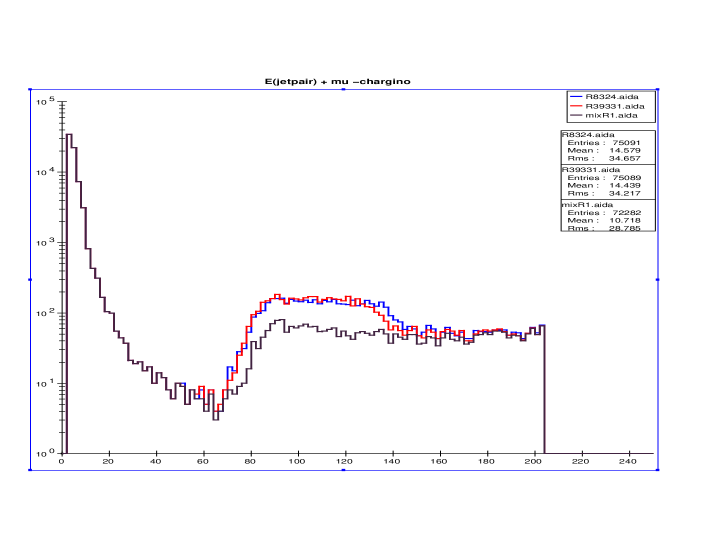
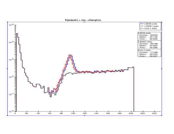
Figure 55: Jet-pair energy distribution: the number of events/2 GeV bin after imposing the full set of cuts discussed in the text for the 2-jet $+\mu$ channel with $\Delta m_{\tilde{\chi}}<M_{W}$ for representative models which are visible in this channel. RH(LH) beam polarization is employed in the top(bottom) panel, assuming an integrated luminosity of 250 fb^-1 for either polarization. The SM background is shown as the black histogram.

We now compare these results to those for the case of the well-studied benchmark point SPS1a’. Figures 56 and 57 display the jet pair invariant mass spectrum and energy distribution, respectively, for both polarization choices. The chargino in this model decays to an on-shell $W$ boson and has a large production cross section; both of these features are observable in the Figures. The signal for this model is clearly visible above the SM background and there is a peak at $M_{jj}\simeq M_{W}$ in the invariant mass distribution.

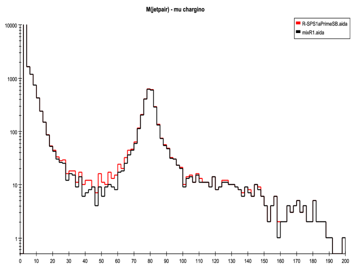
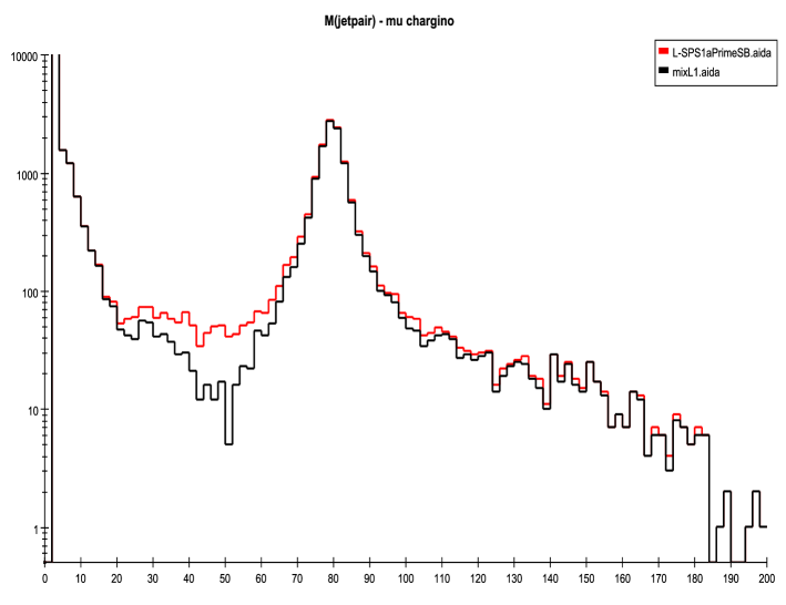
Figure 56: Jet-pair invariant mass distribution: the number of events/2 GeV bin after imposing the full set of cuts discussed in the text for the benchmark model SPS1a’. RH(LH) beam polarization is employed in the top(bottom) panel, assuming an integrated luminosity of 250 fb^-1 for either polarization. The SM background is shown as the black histogram.

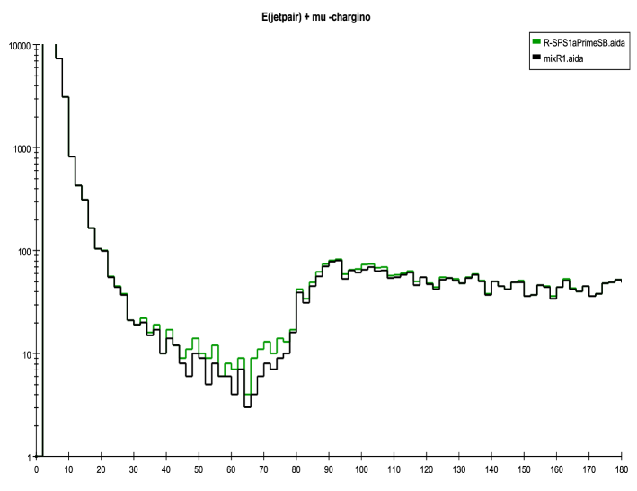
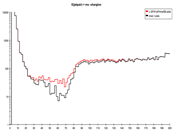
Figure 57: Jet-pair energy distribution: the number of events/2 GeV bin after imposing the full set of cuts discussed in the text for the benchmark model SPS1a’. RH(LH) beam polarization is employed in the top(bottom) panel, assuming an integrated luminosity of 250 fb^-1 for either polarization. The SM background is shown as the black histogram.

V.2 Radiative Chargino Production

As was pointed out by Gunion and collaborators Gunion:2001fu ; Chen:1995yu ; Chen:1999yf (see also Riles et al.Riles:1989hd ), in the case where $\Delta m_{\tilde{\chi}}$ is in the approximate range 0.1 GeV $\mathrel{\mathchoice{\lower 3.01385pt\vbox{\halign{$\matth\displaystyle\hfil#\hfil$\cr<\crcr\sim\crcr}}}{\lower 3.01385pt\vbox{\halign{$\matth\textstyle\hfil#\hfil$\cr<\crcr\sim\crcr}}}{\lower 3.01385pt\vbox{\halign{$\matth\scriptstyle\hfil#\hfil$\cr<\crcr\sim\crcr}}}{\lower 3.01385pt\vbox{\halign{$\matth\scriptscriptstyle\hfil#\hfil$\cr<\crcr\sim\crcr}}}}\Delta m\mathrel{\mathchoice{\lower 3.01385pt\vbox{\halign{$\matth\displaystyle\hfil#\hfil$\cr<\crcr\sim\crcr}}}{\lower 3.01385pt\vbox{\halign{$\matth\textstyle\hfil#\hfil$\cr<\crcr\sim\crcr}}}{\lower 3.01385pt\vbox{\halign{$\matth\scriptstyle\hfil#\hfil$\cr<\crcr\sim\crcr}}}{\lower 3.01385pt\vbox{\halign{$\matth\scriptscriptstyle\hfil#\hfil$\cr<\crcr\sim\crcr}}}}2$ GeV, the dominant decay mode of the charginos is into soft pions plus the LSP (which appears as missing energy), as shown in Fig. 40. The dominant SM background to this final state is from $\gamma\gamma$ interactions and has an enormous event rate. If $\Delta m_{\tilde{\chi}}<m_{\pi}$, however, the dominant chargino decay is leptonic, $\tilde{\chi}_{1}^{\pm}\rightarrow e^{\pm}\nu_{e}\tilde{\chi}^{0}_{1}$, and does not pose a problem for detection as this essentially results in a charged stable-particle search. In this subsection, we discuss the radiative chargino search where the hard photon emitted in the process $e^{+}e^{-}\to\tilde{\chi}^{+}_{1}\tilde{\chi}^{-}_{1}\gamma$ is tagged. Unlike the other chargino signatures we consider, the strength of this signal is not very dependent on the mass splitting between the lightest chargino and the LSP neutralino.

V.2.1 Event Generation

An immediate issue in performing the search for radiative chargino production is that we find PYTHIA underestimates the rate and energy distribution of hard photon emission from the final state charginos. Thus we use CompHEP Boos:2004kh to generate the $e^{+}e^{-}\to\tilde{\chi}^{+}_{1}\tilde{\chi}^{-}_{1}\gamma$ (as well as $e^{+}e^{-}\to\tilde{\chi}^{+}_{1}\tilde{\chi}^{-}_{1}$) events from the explicit (tree-level) matrix elements.

In particular, we find that PYTHIA with default ISR and FSR options yields a lower cross section for chargino production with an associated photon than does CompHEP. This is illustrated in Fig. 58 where we display the cross section for $e^{+}e^{-}\to\tilde{\chi}^{+}\tilde{\chi}^{-}\gamma$ in one of the AKTW models (labelled as model 13348) as a function of photon transverse momentum. For this model (where the $\tilde{\chi}^{+}_{1}$ has a mass of $\simeq 124$ GeV) the cross section computed by PYTHIA is about $20$% smaller than the CompHEP cross section for all values of $p_{T}$. In examining the MSSM parameter space further, we find points where the PYTHIA generated cross section can be as low as $50$% of that calculated via CompHEP; for the models considered in this paper, the PYTHIA cross section is generally $80-90$% of that from CompHEP. As CompHEP uses an exact (tree-level) matrix element calculation, it is presumably more accurate. Therefore we use CompHEP when calculating the cross sections for radiative chargino production in each of our models and to generate the events for this process.

CompHEP does not allow one to set an arbitrary beam polarization. However, one may set the electron beam polarization to be, for example, purely left-handed, by effectively inserting the relevant projection operator into the expression for the matrix element. Thus we can calculate the desired cross sections and generate events for each of the two initial helicity states that we consider here. For each pure initial helicity state we generate two large event files and find the relevant cross sections. We then choose the correct number of events for each of our two partial electron beam polarizations (80% left-handed and 80% right-handed) and pipe this through our analysis as described in Section III.

CompHEP includes the option of using a beamstrahlung spectrum calculated from the beam dimensions and the number of particles per bunch. However, for consistency with the rest of our signal and background, we must use the same beam spectrum as described above. To implement this spectrum in CompHEP, we read in the beamspectrum as generated by GuineaPig Guinea . We checked that the normalization was correct by comparing the cross sections for $e^{+}e^{-}\to t\bar{t}$ as generated by our modified CompHEP code and by PYTHIA.

In calculating the cross section and generating events for the $\tilde{\chi}^{+}_{1}\tilde{\chi}^{-}_{1}\gamma$ final state, we demand that the transverse momentum of the photon be greater than 5 GeV. This cut is much softer than that we apply in our analysis with the detector simulation; we do not wish to eliminate the possibility of low $p_{T}$ signal events passing the final $p_{T}$ cut due to mismeasurement. We do, however, need to apply a cut at this stage for the purpose of regularization.

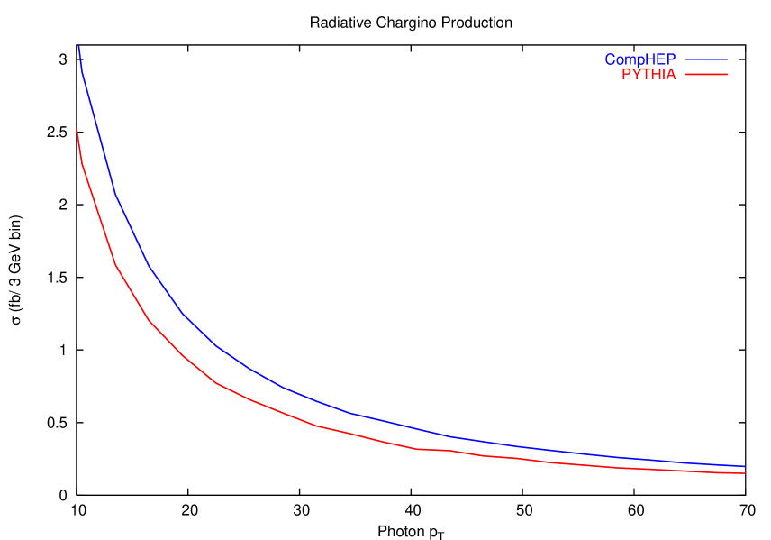
Figure 58: Comparison of the cross section for the pair production of the lightest chargino with an associated photon as a function of the photon transverse momentum as calculated by PYTHIA (red, bottom curve) and by CompHEP (blue, top curve) in one of the AKTW models where $m_{\tilde{\chi^{+}}}=124$ GeV.

V.2.2 Analysis

In our analysis, we tag on a high-$p_{T}$ photon, produced by the signal either off the initial state electron-positron pair, or radiated off of one of the charginos. We apply the following kinematical cuts as suggested in Gunion:2001fu ; Abbiendi:2002vz :

1. There be exactly one photon in the event with $p_{T}>0.035\sqrt{s}$ and no other charged tracks within 25 degrees. This isolation cut removes most of the two-$\gamma$ background.

2. There be no identified (i.e., above 142 mrad) electrons or muons in the event. Although this cut slightly reduces the signal, we find it dramatically decreases the background from $\gamma\gamma$ and $e^{\pm}\gamma$ events. For the signal, we see from Fig. 40 that the branching fraction of charginos to electrons or muons is less than $30-40\%$ in the relevant $\Delta m_{\tilde{\chi}}$ range.

3. We demand that the number of charged tracks be in the range 1 to 11. Note that below 142 mrad the detector only observes clusters of energy, however, we nonetheless treat clusters on the same footing as tracks. This cut removes high-multiplicity events. In particular, the removal of high-multiplicity events restricts this analysis to the range of $\Delta m_{\tilde{\chi}}$ that we are targeting in this analysis. Models with larger values of $\Delta m_{\tilde{\chi}}$ generate harder partons in the chargino decay that radiate more gluons and hence result in more tracks.

4. We demand that the photon energy and the energy of the remaining visible particles satisfy $E_{\mbox{\tiny vis, other particles}}-E_{\gamma}<0.35\sqrt{s}$. This cut further reduces the two-$\gamma$ background. It also serves to restrict this analysis to the relevant range of $\Delta m_{\tilde{\chi}}$, as the amount of visible energy increases with $\Delta m_{\tilde{\chi}}$.

5. We demand that the ratio of total visible transverse momentum to transverse energy satisfy $\frac{p_{T\,\mbox{\tiny vis}}}{E_{T\,\mbox{\tiny vis}}}>0.4$ and that the ratio of total visible transverse momentum to total momentum be $\frac{p_{T\,\mbox{\tiny vis}}}{p_{\tiny tot\,\mbox{\tiny vis}}}>0.2$. This removes most of the hadronic two-$\gamma$ and $e^{+}e^{-}$ initiated processes.

6. We require that the recoil mass be $M_{\mbox{\tiny recoil}}=\sqrt{s}\sqrt{\left(1-2E_{\gamma}/\sqrt{s}\right)}>160$ GeV. This is the recoil mass of the tagged photon, which should be at least twice the current lower bound on the chargino mass, which we take to be 160 GeV from the approximate 80 GeV lower limit on the chargino mass from LEP II Yao:2006px .

After applying these cuts we examine the recoil mass of the tagged photon,

$$M_{\mbox{\tiny recoil}}=\sqrt{s}\sqrt{\left(1-2E_{\gamma}/\sqrt{s}\right)}\,.$$ (25)

The dominant remaining SM background again arises from the reaction $e^{+}e^{-}\rightarrow l^{-}\bar{\nu}_{l}\nu_{l^{\prime}}{l^{\prime}}^{+}$ as illustrated in Fig. 59.

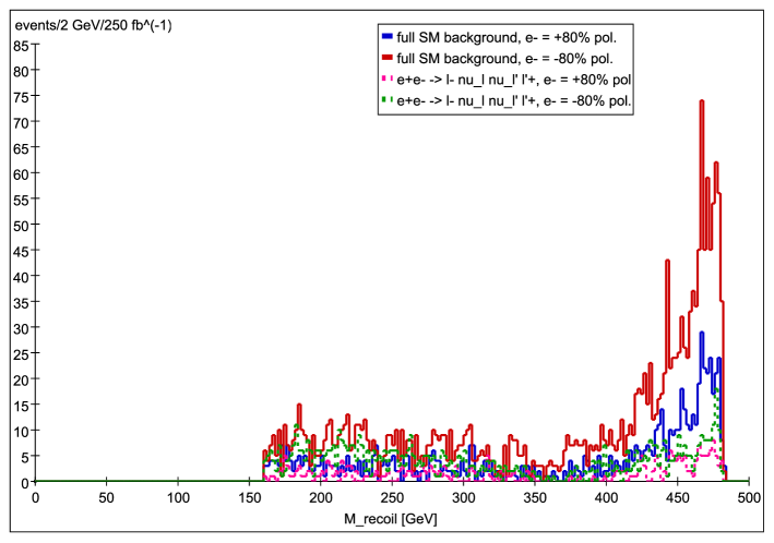
Figure 59: Recoil mass of the tagged photon for the SM background to radiative chargino production after the cuts listed in the text have been applied. This is generated from $250\mbox{ fb}^{-1}$ of SM events with 80% right-handed (solid blue line) and 80% left-handed (solid red line) electron beam polarization and unpolarized positron beam at $\sqrt{s}=500$ GeV. The dotted lines show the main processes contributing to the background, $e^{+}e^{-}\rightarrow l^{-}\bar{\nu}_{l}\nu_{l^{\prime}}{l^{\prime}}^{+}$, for 80% right-handed (dotted pink line) and 80% left-handed electron polarization (dotted green line).

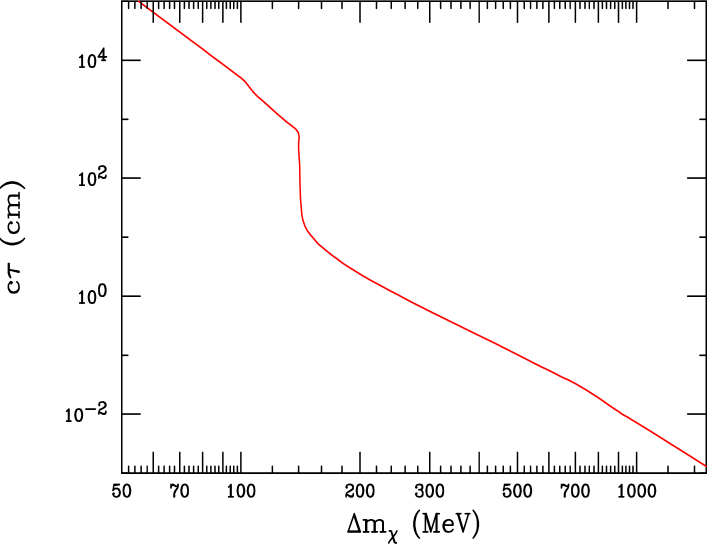
Figure 60: Chargino lifetime as a function of the chargino-neutralino mass splitting, $\Delta m$.

This analysis is designed to only catch charginos in a relatively narrow mass and $\Delta m_{\tilde{\chi}}$ range. If $\Delta m_{\tilde{\chi}}$ is, e.g., greater than $\sim 3-4$ GeV, then the kinematical properties of the average chargino decay may have difficulty satisfying our energy, momentum and multiplicity cuts. If the mass splitting is too small (less than $\sim 0.15$ GeV), then the chargino will have a long lifetime, as shown in Fig. 60, and will decay to at most 2 charged tracks and will not pass the above cuts. Furthermore, if the mass of the chargino is too close to the beam energy ($\mathrel{\mathchoice{\lower 3.01385pt\vbox{\halign{$\matth\displaystyle\hfil#\hfil$\cr>\crcr\sim\crcr}}}{\lower 3.01385pt\vbox{\halign{$\matth\textstyle\hfil#\hfil$\cr>\crcr\sim\crcr}}}{\lower 3.01385pt\vbox{\halign{$\matth\scriptstyle\hfil#\hfil$\cr>\crcr\sim\crcr}}}{\lower 3.01385pt\vbox{\halign{$\matth\scriptscriptstyle\hfil#\hfil$\cr>\crcr\sim\crcr}}}}225$ GeV), then not only will the cross section be phase space suppressed, but it will be almost impossible for the signal to pass the required photon $p_{T}$ cut. Depending on exactly how these kinematic boundaries are chosen, we find that only $\sim 26$ of the 53 AKTW models with kinematically accessible charginos at $\sqrt{s}=500$ GeV have these necessary properties. From this analysis we find that there are only 14 models which are observable in the radiative channel (for either beam polarization) over the SM background with a significance ${\cal S}>5$. Note that although the backgrounds are larger in the LH sample than with RH beams, as is usual, the chargino signal in this case is far larger (by approximately a factor of 9) in the LH sample. This is because for small $\Delta m_{\tilde{\chi}}$ the charginos in these models are mostly wino in content. This is illustrated in Fig. 61 which shows our analysis results for a number of sample representative models with either beam polarization. Model 38239, which is shown in this Figure, provides a nice example of a case that is missed by this analysis; this model has $\Delta m_{\tilde{\chi}}=0.45$ GeV while $m_{\tilde{\chi}_{1}^{+}}=239.75$ GeV and thus has little remaining phase space to allow for the emission of a hard photon with $p_{T}\geq 17.5$ GeV.

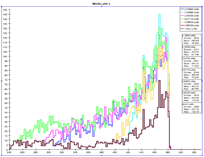
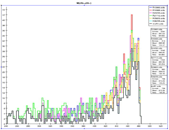
Figure 61: Recoil mass distribution for chargino pair production in the AKTW models from the photon tag analysis: number of events/2 GeV bin assuming an integrated luminosity of 250 fb^-1 for both LH (top panel) and RH (bottom panel) electron beam polarization.

The benchmark model SPS1a’ also leads to a reasonable signal excess in this channel as shown in Fig. 62. However, in this case, this is not the result of a small $\tilde{\chi}_{1}^{\pm}-\tilde{\chi}_{1}^{0}$ mass difference, which is 86 GeV in this model, but rather the signal in this channel for is a ‘fake’ induced by $\tilde{\chi}_{2}^{0}$ production. As discussed above for some of the AKTW models, the observed signal in this case is actually a feed down from the production of other, perhaps more massive, states in the SUSY spectrum as well as from radiative associated $\tilde{\chi}_{1}^{0}\tilde{\chi}_{2}^{0}$ production. However, the $\tilde{\chi}_{1}^{\pm}$ in SPS1a’ is already clearly observable in the other channels discussed above. We generally find that the fake contamination in the radiative channel is less than $30\%$ and is quite a bit smaller in many cases.

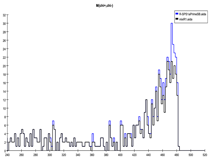
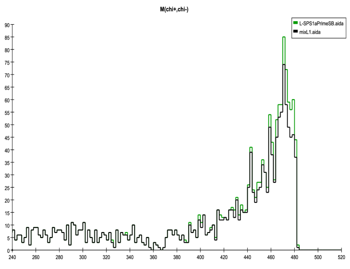
Figure 62: Recoil mass distribution for chargino pair production in SPS1a’ from the photon tag analysis: number of events/2 GeV bin assuming an integrated luminosity of 250 fb^-1 for both LH (top panel) and RH (bottom panel) electron beam polarization.

V.3 Very Close Mass Case

As mentioned above, when $\Delta m_{\tilde{\chi}}<m_{\pi}$ the decay length of the chargino is long compared with the detector size, as is shown in Fig. 60. In this case, chargino production may be detected by searching for two massive, essentially stable, charged particles that traverse the full detector. Seven of the 53 AKTW models with kinematically accessible charginos at the 500 GeV ILC fall into this category. To perform this search we demand:

1. There be only 2 massive charged tracks in the event.

2. There be no tracks, or energy clusters, within 100 mrad of the beam.

3. $\beta=\frac{p}{E}<0.93$ for both charged tracks. (This value is based on constraints from LEPII Yao:2006px .)

4. The energy of the two tracks satisfy $\sum\limits_{i=1}^{2}E_{i}>0.75\sqrt{s}$.

The last two cuts remove most of the background from the production of muons. After these cuts are imposed, the remaining background should be small, aside from detector fakes and possible tails from muon production due to detector smearing. We then study the $\beta=\frac{p}{E}$ spectrum for both charged tracks and look for excesses in the region of low $\beta$.

In this analysis we search for stable charged tracks in the final state whose energy can be reconstructed via a $dE/dx$ measurement. $\beta=p/E$ should be significantly less than 1, which would allow us to easily distinguish such tracks from those produced by Standard Model particles. However, in the current public version of org.lcsim lcsim , $dE/dx$ is not yet implemented. We therefore employ a cheat algorithm, and smear, by a random amount, the energy of all final state tracks which we take from the PYTHIA input before detector simulation. The width of a random Gaussian fluctuation should mimic the resolution obtainable from a more realistic TOF (Time Of Flight) or $dE/dx$ measurement. There is not yet full agreement among the ILC detector experts as to the attainable precision which may be possible in the determination of $\beta$ private , so we perform two analyses, one with a 5% and one with a 10% assumed resolution on $\beta$. (Note that an energy smearing of $5(10)\%$ translates into a resolution on $\beta$ of roughly $5(10)\%$.) We note that both the ATLAS and CMS detectors have excellent $\beta$ resolutions of $5(3)\%$ lhcbeta , respectively, and we anticipate that any ILC detector should have a comparable precision as demonstrated in Ref. Martyn:2007mj .

As shown in Fig. 63, the background is indeed negligible for an energy smearing of 5%. However, some SM background from Bhabha scattering with missing energy due to initial state radiation and beamstrahlung where the forward photon is not detected, leaks into the analysis when an energy smearing of 10% is assumed. The background displayed in Fig. 63 is almost entirely due to this process. Nevertheless, we expect the ILC to have an energy resolution better than 10%, so this background source should not be a problem.

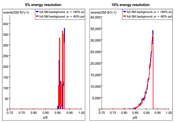
Figure 63: $\beta=p/E$ distribution of the SM background after the kinematic cuts listed in the text have been imposed. This is generated from $250\mbox{ fb}^{-1}$ of SM events generated with 80% right-handed (solid blue line) and 80% left-handed (solid red line) electron beam polarization and unpolarized positron beam at $\sqrt{s}=500$ GeV. In the Figure in the left panel, we assume an energy resolution of 5%, the Figure on the right is for an energy resolution of 10%.

Out of the 53 AKTW models with kinematically accessible chargino pairs, only 7 have values of $\Delta m_{\tilde{\chi}}<m_{\pi}$ and have effectively stable charginos as far as collider detector measurements are concerned. As in the previous analysis for radiative chargino production, the backgrounds are similar for both polarizations, however the chargino production cross sections for these models are about a factor of 9 larger in the case of LH polarization than in the RH case. This is because charginos with small values of $\Delta m_{\tilde{\chi}}$ are mostly wino in the AKTW models, corresponding to large values of the $\mu$ parameter. Figure 64 shows these 7 models for both values of the assumed $\beta$ resolution and we see that in either case all of these models are clearly visible above background.

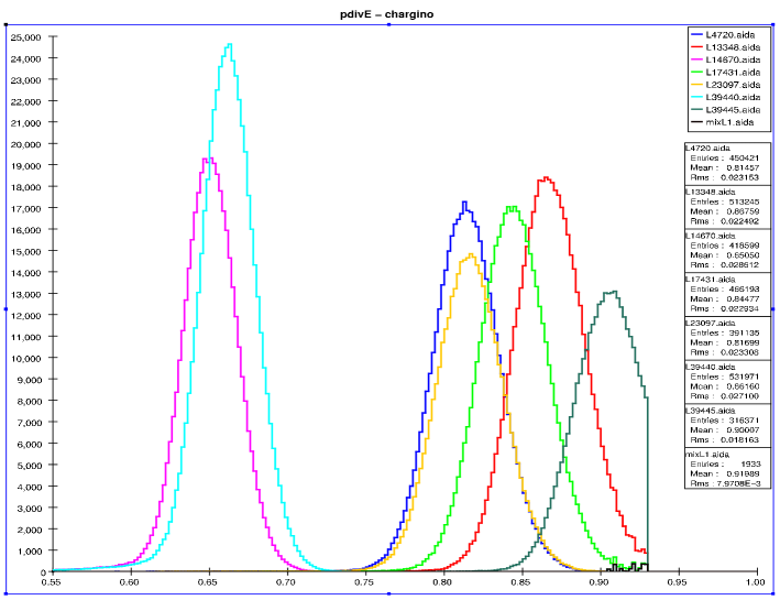
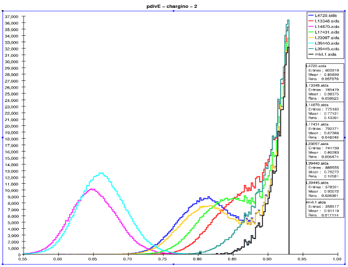
Figure 64: Velocity (=$\beta=p/E$) distribution for long-lived charginos assuming an integrated luminosity of 250 fb^-1 and LH electron beam polarization. The top(bottom) panel corresponds to a resolution of $5(10)\%$ on $\beta$.

Of course this search will not just find charginos, but will also detect any sufficiently long-lived charged particles in the kinematically accessible mass range. In fact, out of the 28 AKTW models with kinematically accessible $\tilde{\tau}$’s, we find 3 models (labelled as 207, 27285 and 29334) which have staus with very long lifetimes; in one of these cases (27285) the $\tilde{\tau}$ is the NLSP. Such a situation can occur, e.g., in gauge mediation, where the $\tilde{\tau}$ will decay with a very long lifetime by emitting a gravitino Ambrosanio:1997rv . Of course in such a model $\tilde{\chi}_{1}^{0}$ is not the actual LSP; thus the cosmology is non-standard, but viable. With the above analysis, these models should also lead to observable signals in this channel.

These two possible candidate for stable charged particles are easily distinguished by their angular distributions, i.e., spin-0 vs. spin-1/2, as well as by their response to the various electron beam polarizations as we will see below.

A similar search can be performed in the case of the three models with long-lived staus; the results are seen in Fig. 65. Recall that in the case of stau pair production the cross section is not only controlled by the $\tilde{\tau}$ mass but also by the $\tilde{\tau}_{L,R}$ mixing angle which governs the stau coupling to the $Z$ boson. Note that the event rates shown here are significantly lower than those of the long-lived charginos and so the SM background is potentially more serious. It is clear, however, that in the case of a $5\%$ resolution on $\beta$ the staus in these 3 models will be observable; the situation is more difficult to assess by eye in the case of only a $10\%$ resolution. A detailed statistical study, however, shows that these 3 stau models will lead to signals at the level of significance $>5$ for both choices of the electron beam polarization and for either assumed value of the $\beta$ resolution. We observe that stau production in these 3 special models with both LH and RH beam polarization lead to comparable cross sections.

We note that there are no long-lived charged particles in the case of SPS1a’.

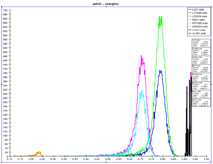
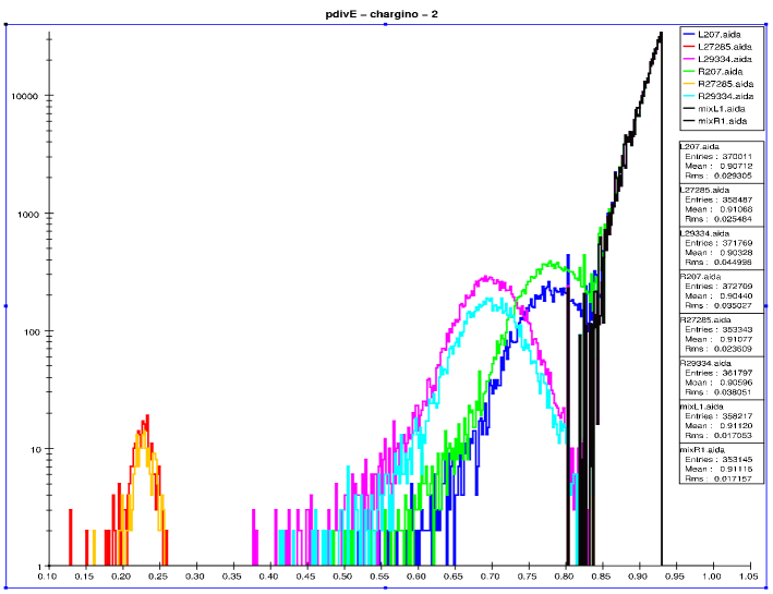
Figure 65: Velocity(=$\beta=p/E$) distribution for long-lived staus assuming an integrated luminosity of 250 fb^-1 and for both electron beam polarizations as labelled. The top(bottom) panel corresponds to a resolution of $5(10)\%$ on $\beta$.

V.4 Summary of Chargino Analyses

Here, we collect and summarize the results of the various chargino analyses presented in this section. We remind the reader that the set of AKTW models contain 53 models with kinematically accessible charginos at the 500 GeV ILC. The critical parameter that determines the open decay channels for the chargino, and hence governs the appropriate search analysis, is $\Delta m_{\tilde{\chi}}$, the mass difference between the lightest chargino and the $\tilde{\chi}_{1}^{0}$ LSP. Of the 53 models, 7 have values of $\Delta m_{\tilde{\chi}}$ small enough to render the lightest chargino essentially stable and it traverses the full detector before it decays. These models are visible in our stable charged particle search. An additional 7 models have chargino-LSP mass differences in the range $\Delta m_{\tilde{\chi}}<1$ GeV, and result in final states with large values of missing energy plus several soft pions. These models are targeted by our radiative chargino analysis. Thirty-seven of the models have mass differences in the range $1<\Delta m_{\tilde{\chi}}<6$ GeV and the charginos decay into off-shell $W$ bosons. For this region, we designed a multi-pronged search strategy using 11 observables in 3 decay channels (missing energy + $\mu\mu$, 2 jets $\mu$, 4 jets). Lastly, 2 of the models have $\Delta m_{\tilde{\chi}}>M_{W}$ and in this case the charginos decay into on-shell $W$ bosons. We developed only one search analysis here, utilizing the 4-jet mode, and found this to be a very clean channel for detecting chargino production.

A summary of how many models are visible above the SM background for each observable in our chargino search analyses is presented in Table 3. Here, we employ, as always, our visibility criteria that the signal significance ${\cal S}>5$. We see that the channel with the mixed final state of 2-jets + muon + missing energy and the missing energy observable in the 4-jet + missing channel yield the highest number of observable models and thus are the best channels for detecting chargino production in the randomly generated AKTW models.

Observable	Visible with RH	Visible with LH
$E_{jj}^{\mbox{\tiny}on-shell}$	2	2
$E_{\mu\mu}$	12	10
$E_{\mbox{j}et-pair}-\mu$	26	35
$E_{\mbox{j}et-pair}-\mu$, $m_{\tilde{\chi}^{0}_{1},\mbox{\tiny min}}=100$ GeV	0	0
$M_{\mbox{j}et-pair}-\mu$	23	35
$M_{\mbox{j}et-pair}-\mu$, $m_{\tilde{\chi}^{0}_{1},\mbox{\tiny min}}=100$ GeV	0	0
ME(4jets)	9	30
ME(4jets), $m_{\tilde{\chi}^{0}_{1},\mbox{\tiny min}}=100$ GeV	4	34
ME(4jets), additional $p_{T}$ cut	3	2
$M_{\mbox{j}et-pairs}$	2	4
$M_{\mbox{j}et-pairs}$, $m_{\tilde{\chi}^{0}_{1},\mbox{\tiny min}}=100$ GeV	2	2
$M_{\mbox{j}et-pairs}$, additional $p_{T}$ cut	3	2
Radiative Production	14	14

Table 3: Number of models that are visible above the SM background with a significance ${\cal S}>5$ in each observable at $\sqrt{s}=500$ GeV with 250 ${\rm fb}^{-1}$ of integrated luminosity for each electron beam polarization.

Figure 66 displays the location of each AKTW model with $\Delta m_{\tilde{\chi}}<M_{W}$ in the $\Delta m_{\tilde{\chi}}-$ chargino mass plane. The color coding of the model marker indicates whether it is observable in any of our analyses for either beam polarization as labelled in the Figure caption. The location of the various model points in this plane reveals the kinematic properties targeted by each search technique. For example, the radiative production analysis captures the models with low $\Delta m_{\tilde{\chi}}$ as it was designed to do, and also detects charginos that are light enough to be produced with a hard photon. Here, we see that all 7 of the essentially stable charginos are captured by our stable charged particle search, 3 models are only observable via radiative chargino production, 11 models are visible in both the radiative production channel and at least one of the off-shell $W$ analyses, while 26 models are detectable in at least one of the off-shell $W$ analyses but not in radiative production. 4 out of the 53 AKTW models are not observable in any of our analysis channels. However, each of these 4 models have a lower cross section due to phase space suppression.

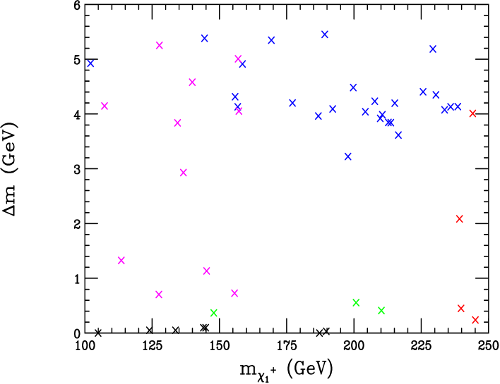
Figure 66: Distribution of the chargino-LSP mass difference versus the chargino mass for the AKTW models with $\Delta m_{\tilde{\chi}}<6$ GeV for the $\tilde{\chi}_{1}^{\pm}$ states that are accessible at $\sqrt{s}=500$ GeV. The blue crosses represent models that are observable in our suite of analysis channels based on the $\tilde{\chi}_{1}^{\pm}$ decay via off-shell $W$ bosons. The green crosses correspond to models that are only visible in the radiative chargino production analysis channel, while the magenta ones represent models that yield observable signals in both the radiative and off-shell $W$ channels. The black crosses are models that are visible in the stable chargino analysis. The red points are the 4 models where the $\tilde{\chi}_{1}^{\pm}$ state is not observable in any of our analysis channels, essentially due to phase space restrictions.

VI Neutralino Production

The neutralino sector of the MSSM is the most complex as the mass eigenstates are admixtures between the Bino, neutral Wino, and two neutral Higgsino weak states. Neutralinos, $\tilde{\chi}_{i}^{0}$, can be pair produced in $e^{+}e^{-}$ collisions via two distinct mechanisms: $s-$channel $Z$ boson exchange can make a neutral Wino plus a Higgsino, while $t,u-$channel selectron exchange can produce Binos and neutral Winos in all combinations. These mechanisms ensure that all of the ten possible processes $e^{+}e^{-}\to\tilde{\chi}_{i}^{0}\tilde{\chi}_{j}^{0}$ are potentially accessible with rates depending upon the sparticle masses and the various mixing angle factors. At a $\sqrt{s}$=500 GeV machine, it is likely that only the first one or two of these states will be kinematically accessible and this is indeed the case for the wide selection of AKTW models analyzed here as shown in Fig. 8 and Table  1. If the mass separation between $\tilde{\chi}_{1}^{0}$ and $\tilde{\chi}_{2}^{0}$ is sufficiently large, then the decay channel $\tilde{\chi}_{2}^{0}\to Z\tilde{\chi}_{1}^{0}$ may lead to a clear signal if the $Z$ boson is not too far off-shell. Unfortunately, in the models examined here, if $\tilde{\chi}_{2}^{0}$ is sufficiently light to be produced it is very close in mass to $\tilde{\chi}_{1}^{0}$ and we find that such decays are almost impossible to observe. That being the case, we only consider $\tilde{\chi}_{1}^{0}$ pair production with a radiated photon, as well as $\tilde{\chi}_{1}^{0}\tilde{\chi}_{2}^{0}$ associated production in the discussion below. Recall that $\tilde{\chi}_{1}^{0}$ is the only accessible MSSM particle in many of the AKTW models.

It is important to consider the weak eigenstate mixture of the $\tilde{\chi}_{1}^{0}$ in our set of models; this is shown in Fig. 67, where it is interesting to observe that the lightest neutralino is mostly a pure weak eigenstate.

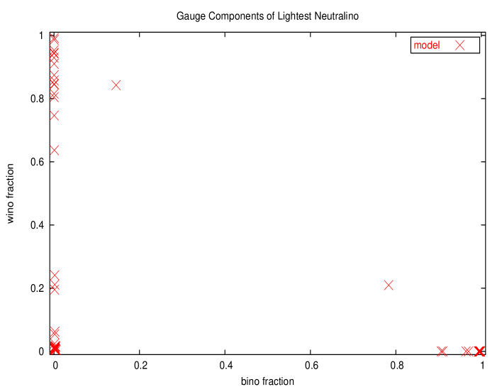
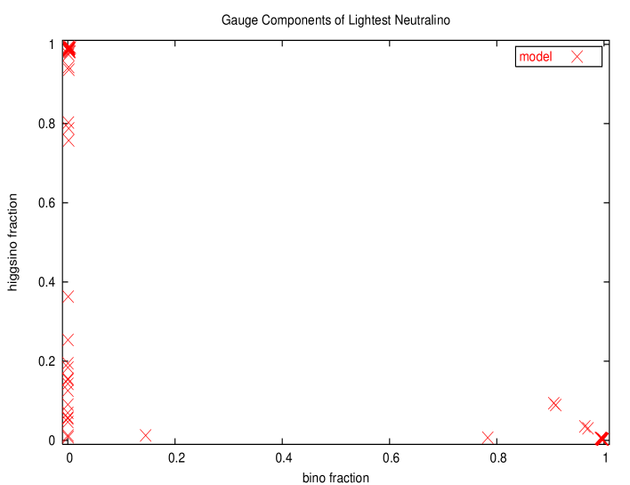
Figure 67: The composition of the lightest neutralino in the 242 AKTW models.

VI.1 $\tilde{\chi}_{2}^{0}\tilde{\chi}_{1}^{0}$ Associated Production

In order to get a handle on the neutralino sector, it is important to consider the associated production of neutralinos, i.e., $e^{+}e^{-}\to\tilde{\chi}_{2}^{0}\tilde{\chi}_{1}^{0}$, which proceeds by $Z$ boson exchange in the $s$-channel via the Wino and Higgsino content of the $\tilde{\chi}_{1,2}^{0}$ and by selectron exchange in the $t,u$-channels via their corresponding Wino and Bino content. The cross section for this process is thus sensitive to the mixing in the neutralino sector as well as to the masses of the exchanged $\tilde{e}_{L,R}$. Note that if the selectrons are heavy, as is the case in many of the AKTW models, then the $s$-channel transition dominates; in this situation the associated production process will be suppressed if either or both of the $\tilde{\chi}_{2}^{0}$ or $\tilde{\chi}_{1}^{0}$ have a large Bino content, which as we saw above, is a relatively common occurrence in the models considered here.

At $\sqrt{s}=500$ GeV, 46/242 of the AKTW models have the final state $\tilde{\chi}_{2}^{0}\tilde{\chi}_{1}^{0}$ kinematically accessible. The state $\tilde{\chi}_{2}^{0}$ can decay in several ways depending on the mass spectrum details in the gaugino sector. A mode which is always present and yields a relatively clean signature is $\tilde{\chi}_{2}^{0}\to\tilde{\chi}_{1}^{0}Z/H$, with the $Z/H$ being on- or off-shell depending on the $\tilde{\chi}_{2}^{0}-\tilde{\chi}_{1}^{0}$ mass difference. Certainly, this channel will be easier to observe in the on-shell case since the invariant mass distribution of the visible particles in the final state will be peaked at the $Z/H$ mass. In either case, we consider the decay modes $Z,H\to jj$, with the jets not flavor tagged, as well as the leptonic modes $Z\to\mu^{+}\mu^{-},e^{+}e^{-}$. In order to access the viability of this channel, we examine in Fig. 68 the mass splitting between the first two neutralino states for the 46 models where this production mechanism is kinematically accessible. Here, we see that for most models the mass splitting is rather small; only 8 of these models have neutralino mass splittings larger than $M_{Z}$ and 13 have mass differences larger than 20 GeV. It is unlikely that any of the other remaining models will produce hard enough jets and/or leptons to pass the analysis cuts or be visible above background. For the models with the larger mass differences, we stress again that their signal rates will be controlled by both the selectron masses and the Bino content of the two neutralinos. The dominant background we contend with arise from, e.g., $e^{+}e^{-}\to ZZ\to jj/\ell^{+}\ell^{-}+\nu\bar{\nu}$, $\gamma e\to\nu W$ with $W\to jj$, as well as $\gamma\gamma\to\ell^{+}\ell^{-}$.

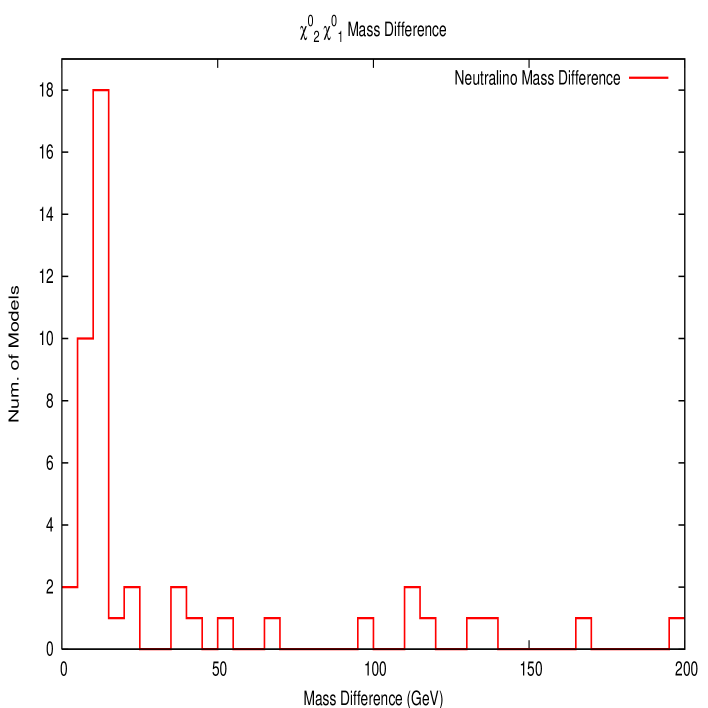
Figure 68: $\tilde{\chi}_{2}^{0}-\tilde{\chi}_{1}^{0}$ mass difference for the 46 AKTW models which have $\tilde{\chi}_{2}^{0}\tilde{\chi}_{1}^{0}$ associated production kinematically accessible at $\sqrt{s}=$ 500 GeV.

To reduce the SM background for associated neutralino production, we demand:

1. There be precisely one lepton pair (electrons or muons) or one jet-pair in the event and no other visible particles.

2. The missing energy satisfy $E_{\mbox{\tiny miss}}>300$ GeV. This removes the majority of the background arising from $Z$ and $W$ boson production.

3. The transverse momentum for each lepton or jet satisfy $p_{T}>0.14\sqrt{s}$. This cut removes most of the ubiquitous $\gamma\gamma$ and $e\gamma$ initiated backgrounds.

4. The angle between the lepton or the jet pair be $<95$ degrees. This further reduces the background from $W$ boson production.

We then examine the invariant mass spectrum of the electron-, muon-, or jet-pair. The remaining background after these kinematic cuts are imposed is displayed for the $\mu\mu\,,jj+$ missing energy channels in Figs. 69 and 70; we find that the background for the $e^{+}e^{-}$ final state is qualitatively similar to those for muons.

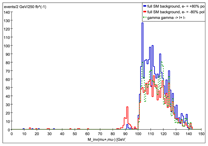
Figure 69: SM background to associated neutralino production for the $M_{inv}(\mu\mu)$ distribution. This is generated for a 250 fb^-1 sample of SM events with $80\%$ RH(solid blue) or LH(solid red) electron beam polarization at $\sqrt{s}=500$ GeV. The dotted green line represents the dominant contribution after the cuts are imposed, $\gamma\gamma\to\ell^{+}\ell^{-}$, which is independent of the beam polarization.

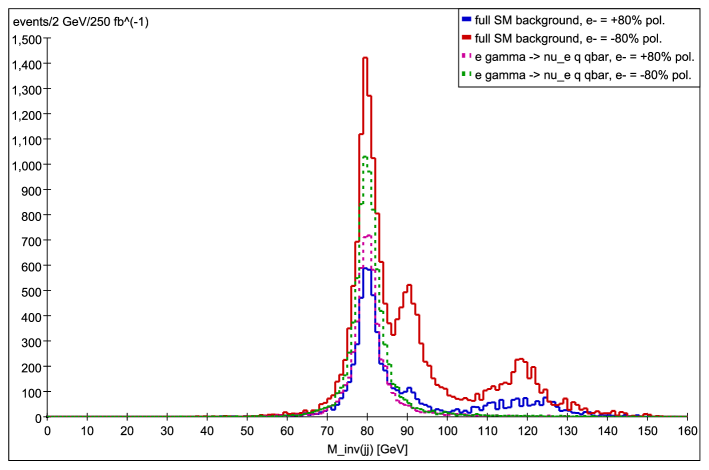
Figure 70: SM background to associated neutralino production for the $M_{inv}(jj)$ distribution. This is generated for a 250 fb^-1 sample of SM events with $80\%$ RH(solid blue) or LH(solid red) electron beam polarization at $\sqrt{s}=500$ GeV. The dominant contribution after the cuts are imposed arise from $\gamma e\to\nu_{e}q\bar{q}$ and are shown by the green(pink) dotted line for LH(RH) beam polarization.

The signal should have a clear peak in the invariant mass spectrum that reconstructs to the $Z$ boson although excesses may also appear elsewhere in the distribution. Note that jet energy resolution is crucial here as some background sources, for example, $e^{-}\gamma\rightarrow\nu_{e}d\bar{u}$ and $e^{-}\gamma\rightarrow\nu_{e}s\bar{c}$, have an invariant mass peak at the $W$ boson mass. Thus the $W$ and $Z$ boson mass peaks must be separable in the 2-jet channel. As is common in many of our analyses, the SM background is far lower with RH electron beam polarization as this suppresses $W$ boson production. Note that we may also have to deal with backgrounds arising from other SUSY production processes that can fake the signals from associated production.

Typical results for these analyses are shown in Fig. 71 for representative AKTW models. In the case of the dijet analysis, three peaks are observable at the masses of the $W$, $Z$ and 120 GeV Higgs boson. Some models lead to small excesses on the $W$ peak while some have excesses at the $Z$; others have excesses at both locations. Five models are found to show a signal with a significance $>5$ in the dijet channel; all these models have small excesses at the $Z$ peak, corresponding to the associated production channel under consideration. Similarly, some models also show some excess at the $W$ peak arising from a different $\tilde{\chi}_{2}^{0}$ decay channel: $\tilde{\chi}_{2}^{0}\to W^{\pm}\tilde{\chi}_{1}^{\mp}$ with $W\to jj,\tilde{\chi}_{1}^{\mp}\to\tilde{\chi}_{1}^{0}+$ very soft jets. This can happen in models with light charginos which have a small mass splitting with the LSP. Unfortunately, the rest of the AKTW models are unobservable, being buried in the dijet case by the enormous $W\to jj$ peak. There are two ways to reduce this background: either decrease the jet pair mass resolution to a value below $30\%/\sqrt{E}$ and/or employ positron polarization to reduce the SM rate for $\gamma e\to W\nu$.

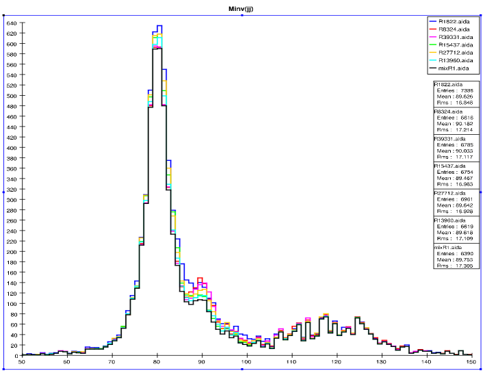
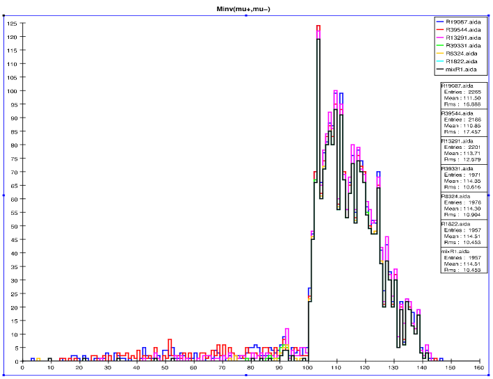
Figure 71: Invariant mass distribution in the dijet (dimuon) channel in the top (bottom) panel from the analysis for associated neutralino production for representative AKTW models: events/2 GeV bin assuming RH polarization and 250 fb^-1 of integrated luminosity. As usual the SM background corresponds to the black histogram.

In the dimuon channel, the signal region is seen to have very little background, however there are also very few signal events. A total of ten AKTW models are found to show an excess over background with a significance $>5$. However, only a few of these excesses can be seen in the $Z$ mass region. Unfortunately, all but 2 of these models are fakes in the sense that they do not have the $\tilde{\chi}_{2}^{0}\tilde{\chi}_{1}^{0}$ channel kinematically accessible; they do, however, all have visible smuons. Some of the signal for models which populate the lower invariant mass region originate from additional sources, such as $\tilde{\chi}_{1}^{+}\tilde{\chi}_{1}^{-}$, or even $\tilde{\chi}_{3}^{0}\tilde{\chi}_{1}^{0}$, production. It would appear from these results that perhaps the cuts employed in this analysis are too strong even though the signal region is essentially background free. However, we find that relaxing the cuts, even just slightly, overwhelms the signal region by background. We have not found a set of cuts that allows more of the signal to be visible over background in this channel. A similar situation happens for LH electron beam polarization. While some models lead to observable signals in the dimuon channel, they are all fakes in the case of either polarization and the apparent signal is due to feed down from other SUSY sources. In the $e^{+}e^{-}$ channel, 7 models are observable with a significance $>5$, however only one of them is not a fake as illustrated in Fig. 72. We note that there are fewer fake signals in the dijet channel.

Thus at this level of statistics, these $jj$, $\mu^{+}\mu^{-}$, and $e^{+}e^{-}$ analyses have captured very few of the AKTW models where $\tilde{\chi}_{2}^{0}\tilde{\chi}_{1}^{0}$ is kinematically accessible.

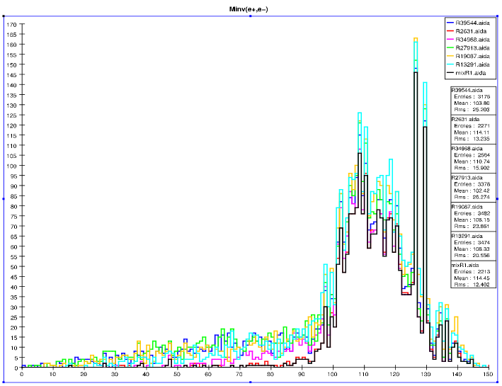
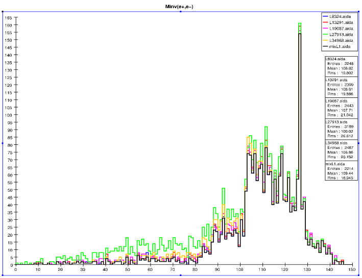
Figure 72: Invariant mass distribution for the dielectron channel in the top (bottom) panel for RH (LH) polarization from the analysis for associated neutralino production for representative AKTW models: events/2 GeV bin assuming 250 fb^-1 of integrated luminosity. As usual the SM background corresponds to the black histogram.

For the conventional benchmark point SPS1a’, associated neutralino production at $\sqrt{s}=500$ GeV can easily proceed as the mass of $\tilde{\chi}_{2}^{0}$ is only 184 GeV. In this case, the $\tilde{\chi}_{2}^{0}-\tilde{\chi}_{1}^{0}$ mass splitting is $\simeq 86$ GeV, i.e., $<M_{Z}$, and thus the signal is not observable in the dijet channel due to the very large SM $W$ boson background. However, a reasonable non-resonant signal excess is observable over background in the substantially cleaner dimuon mode. This is true for either electron beam polarization, however the signal is more strongly observable for the case of LH polarization, as can be seen in Fig. 73. Feed down to this final states from the production of heavier chargino and neutralino states is also present in this model.

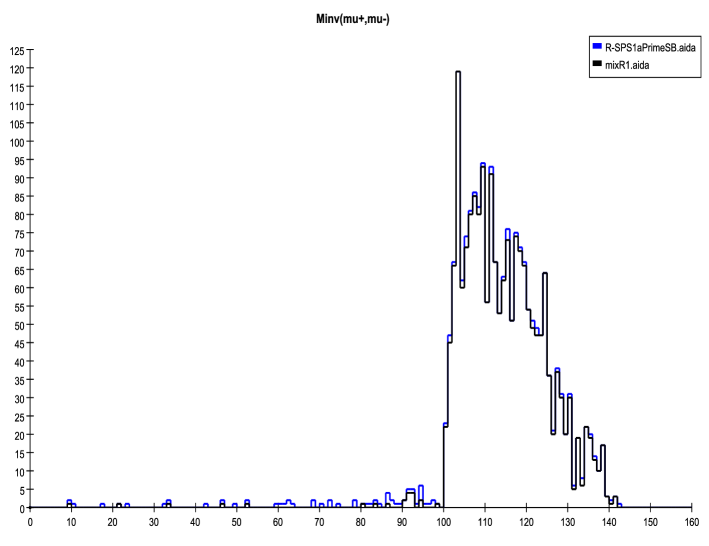
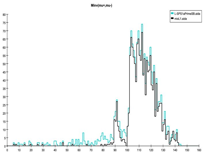
Figure 73: Invariant mass distribution in the dijet (dimuon) channel in the top (bottom) panel from the analysis for associated neutralino production for model SPS1a’: events/2 GeV bin assuming RH polarization and 250 fb^-1 of integrated luminosity. As usual the SM background corresponds to the black histogram.

VI.2 Radiative Neutralino Production

In 91 of the 242 AKTW models the neutralino LSP $\tilde{\chi}_{1}^{0}$ is the only kinematically accessible SUSY particle at $\sqrt{s}=$ 500 GeV. The process $e^{+}e^{-}\to 2\tilde{\chi}_{1}^{0}$ is, by itself, impossible to observe as the final state particles are stable, neutral and weakly interacting. The only way to render $\tilde{\chi}_{1}^{0}$ production observable is to tag it by the emission of a photon off the initial state electrons or off the intermediate $t-$channel selectron; one then looks for an excess of events of the form $e^{+}e^{-}\to\gamma+E_{miss}$. The SM background to such a signature can be quite large and arises mainly from the reaction $e^{+}e^{-}\to\nu\bar{\nu}\gamma$ which occurs through intermediate $W$ and $Z$ boson exchanges. As will be discussed below, beam polarization can play an important role in reducing this dominant component of the SM background, as $W$ bosons couple to electrons in a purely left-handed manner.

As noted above, we employ PYTHIA for the generation of the signal events However, PYTHIA does not take into account photon emission from the virtual $t$-channel selectron in neutralino pair production. Without this contribution to the cross section for $e^{+}e^{-}\to\tilde{\chi}^{0}_{1}\tilde{\chi}^{0}_{1}\gamma$, the signal would always be invisible beneath the background provided by $e^{+}e^{-}\to\nu\bar{\nu}\gamma$. Thus an accurate modelling of the radiative LSP signal at the ILC requires a more sophisticated approach. We therefore use CompHEP to generate the full matrix element for this process, in a manner analogous to that described above in Section 5.2.1 for the radiative chargino analysis. The CompHEP evaluation of the cross section for radiative LSP production uses the complete matrix element and can be up to a factor of 2 larger than that given by PYTHIA and also generally yields harder photons.

We tag on a high-$p_{T}$ photon, which is the sole visible final state particle in the process $e^{+}e^{-}\rightarrow\gamma\tilde{\chi}^{0}_{1}\tilde{\chi}^{0}_{1}$. Clearly, right-handed electron beam polarization should be effective in reducing the background contributions from $W$ boson exchange in $\nu\bar{\nu}\gamma$ production. In fact, after the cuts described below are employed, we find that the RH SM background event rate is about a factor of 7-8 less than that with LH beam polarization. (We note that in the case of $100\%$ electron beam polarization, the LH cross section is almost 50 times larger than that for the RH case.) In contrast, we find that the signal cross sections for the AKTW models follow either one of two patterns: ($i$) the LH and RH polarized cross sections are comparable in magnitude or ($ii$) the RH polarized cross section is far larger than that of the LH case. Thus, for either of these possibilities, RH electron beam polarization is highly favored in order to increase the signal and reduce the background. We will thus limit ourselves to this polarization configuration in our analysis below.

We employ the cuts of Ref. AguilarSaavedra:2001rg , and require:

1. There be exactly one photon and no other visible particle in the event.

2. The photon transverse energy satisfy $E_{T}^{\gamma}=E_{\gamma}\sin\theta_{\gamma}>0.03\sqrt{s}$. Here, $\theta_{\gamma}$ is the angle of the photon with the electron beam axis.

3. The photon be present in the angular region $\cos\theta_{\gamma}<0.9$

4. The total photon energy satisfy the constraint $E_{\gamma}<0.5\sqrt{s}-90$ GeV. This removes radiative return to the $Z$-pole.

We then examine the photon energy distribution and look for a signal in excess of the SM background; some typical results are presented in Fig. 74. Unfortunately, as can be seen from this Figure, $S/B$ is at best $\sim 8-9\%$ for the models shown here. This remains true for all $180$ AKTW models that have kinematically accessible $\tilde{\chi}_{1}^{0}$ states. In many cases $S/B$ is far below the $1\%$ level. However, we find that 17 of the models lead to a signal significance $\cal S$ greater than 5. We note that in 4 of these 17 models, the $\tilde{\chi}_{1}^{0}$ is the only kinematically accessible SUSY particle at $\sqrt{s}=500$ GeV. Of course, a priori, one cannot be certain that the neutralino LSP has been produced and discovered, as this final state may receive sizable signal contributions from other SUSY sources such as $e^{+}e^{-}\to\tilde{\nu}\tilde{\nu}^{*}\gamma$, with $\tilde{\nu}\to\nu\tilde{\chi}_{1}^{0}$. In fact, model 36022, shown in the Figure, is an example of one such case. This renders it difficult to uniquely identify the signal as arising from only the lightest neutralino without further analysis.

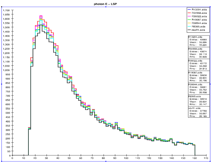
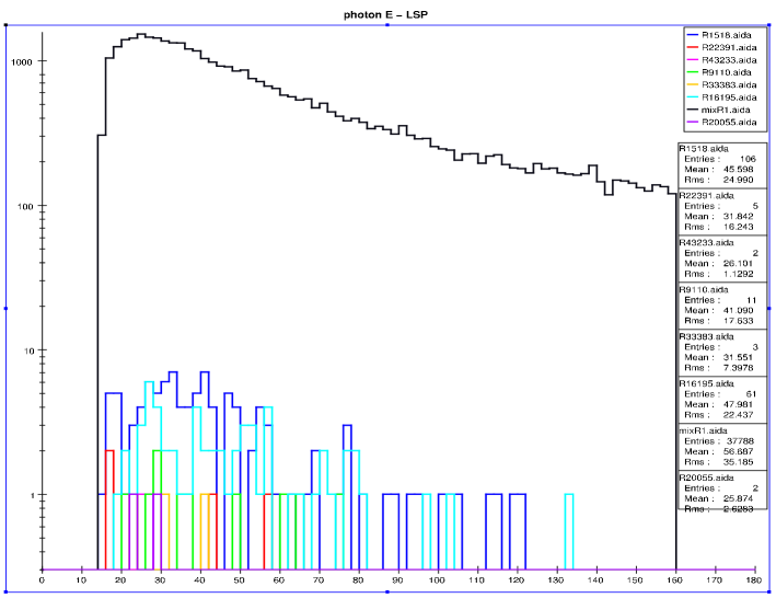
Figure 74: Photon energy spectra for several representative AKTW models from the photon-tagged $\tilde{\chi}_{1}^{0}$ pair production process. Shown is the event rate/2 GeV bin assuming RH electron beam polarization and an integrated luminosity of 250 fb^-1. The black histogram is the SM background. The top panel shows signal plus background for models with larger event rates whereas the bottom panel displays more typical cases with signal and the background now being shown separately.

Of course, increased luminosity or an adjustment of the cuts may make the signal in this channel slightly more visible, but what would be more useful, independently of the choice of cuts, would be to include positron polarization MoortgatPick:2005cw . Having such polarization at the $30(45,60)\%$ level would reduce the background by roughly $\simeq 44(60,73)\%$ in comparison to that with the canonical $80\%$ electron beam polarization assumed in our analysis. The corresponding increase in the signal in the most conservative AKTW model would be $24(36,48)\%$ and thus significant boosts in $S/B$ would result; these increases can be somewhat larger depending upon the parameter values in a particular model.

The observation of radiative neutralino LSP pair production is rather straightforward in the case of the familiar benchmark model SPS1a’, where the LSP is rather light with a mass of only 97.7 GeV. Figure 75 shows that the signal is much larger in this case than in any of the AKTW models. In fact, an excess in the number of events over background can be observed for almost the entire range of the photon energy spectrum. However, some of this excess may be attributed to radiative sneutrino pair production which is reasonably significant in this model Dreiner:2006sb .

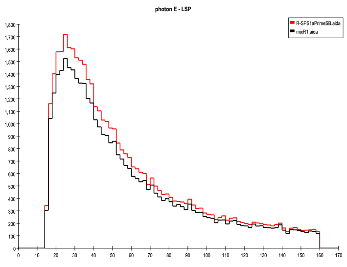
Figure 75: Photon energy spectra for the benchmark model SPS1a’ from the photon-tagged $\tilde{\chi}_{1}^{0}$ pair production process. Shown is the event rate/2 GeV bin assuming RH electron beam polarization and an integrated luminosity of 250 fb^-1. The black histogram is the SM background.

VII Model Visibility and Comparisons

As discussed in the Introduction, before addressing the issue of model differentiation we first need to determine which SUSY particles are visible above the SM background in each of the models under study. In particular we would like to know how many models contain a given SUSY particle that is clearly observable with a significance, $\cal S$, greater than 5 from our Likelihood analysis discussed in Section 3. This information can be obtained by combining the individual results found in Sections 4 through 6; the summary of these analyses in terms of SUSY particle discovery is displayed in Table 4. This Table shows the number of models with a given SUSY particle that we found to yield a visible signal above background in our analysis relevant for that particular SUSY state, as compared to the number of models where the same particle is kinematically accessible. Thus, e.g., the $\tilde{e}_{R}$ is observable in 12 of the 15 models in which it is kinematically accessible. We declare a particle to be visible for a given model if it is kinematically accessible and a signal with ${\cal S}>5$ is observed in the relevant search channel. We note that it is possible that some of these observable signatures may be due to fakes, i.e., the production of other SUSY states; this is certainly true in, e.g., the case of radiative $\tilde{\chi}_{1}^{0}$ production. From this Table we see that for the set of AKTW models the ILC does an excellent job at detecting selectrons and smuons as well as charginos, however, staus are somewhat more problematic, and the neutralino sector appears to be difficult.

Particle	Number Visible
$\tilde{e}_{L}$	8/9
$\tilde{e}_{R}$	12/15
$\tilde{\mu}_{L}$	9/9
$\tilde{\mu}_{R}$	12/15
$\tilde{\tau}_{1,2}$	21/28
$\tilde{\nu}_{e,\mu}$	0/11
$\tilde{\nu}_{\tau}$	0/18
$\tilde{\chi}_{1}^{\pm}$	49/53
$\tilde{\chi}_{1}^{0}$	17/180
$\tilde{\chi}_{2}^{0}$	5/46

Table 4: Number of models, at $\sqrt{s}=500$ GeV, which have a given final state particle visible above the SM background with a significance ${\cal S}>5$ as defined in the text, divided by the number of models where the same particle is kinematically accessible.

We can now combine the results represented in the Table and ask for the total number of models which contain visible sparticles with a signal significance greater than 5. Out of the 85 models which have at least one charged SUSY partner kinematically accessible, we find that 78 have visible sparticle signatures at the ILC. The SUSY particles in the other 7 models are not detectable mainly due to phase space suppression of the SUSY cross sections as discussed in the previous Sections. Of the 96 models which have only stable neutral SUSY partners accessible ($\tilde{\chi}_{1}^{0}$ or $\tilde{\nu}$), 4 of them are observable via the photon tag recoil analysis. Thus, out of all the models with at least one accessible SUSY partner we find that 82/181 lead to detectable signals at the ILC. This corresponds to 82 visible models out of the full set of 242 AKTW models (recall 61 of the models have no SUSY partners accessible at 500 GeV). Surveying all of the models, there is a total of 129 charged sparticles which are kinematically accessible and we find that 111 are visible in our analyses; several more may appear as ‘fakes’.

Using our ILC analyses, we now pairwise compare the models that were found to be indistinguishable at the LHC by AKTW. We recall that out of the original 283 model pairs, 121 were removed from our sample due to the PYTHIA feature which shifted the LSP mass, leaving us with 162 pairs of models to examine. Interestingly, out of these 162 model pairs, 90 have only neutral sparticles kinematically accessible in both models.

In order to compare signals that originate from different models for the observables described in the previous Sections, we perform a $\chi^{2}$ analysis of the generated histogram distributions for the model pairs. To begin, recall that we have generated two complete and statistically independent background sets, $B1$ and $B2$, for all of the individual analyses. Taking the set of pure signal distributions for the two models we wish to compare, $M1$ and $M2$, we add each signal distribution to one of the corresponding background distributions. This forms the combinations $R=M1+B1$ and $S=M2+B2$ for each observable. We then perform a $\chi^{2}$ analysis of the two distributions for each model pair, accounting for the fact that the number of events in each sample can be different:

$$\chi^{2}=\sum_{i}\frac{\left(\sqrt{\frac{S}{R}}R_{i}-\sqrt{\frac{R}{S}}S_{i}\right)^{2}}{R_{i}+S_{i}},$$ (26)

with

$$R=\sum_{i}R_{i}\qquad S=\sum_{i}S_{i}\,.$$ (27)

$R_{i}$ and $S_{i}$ denote the number of events in bin $i$ produced by the two models (plus background) in each observable that we compare. Note that such a $\chi^{2}$ test is somewhat sensitive to the binning of the data, especially since we compare two sets of generated “data” instead of comparing a signal to a theoretical prediction. Note further that the above $\chi^{2}$ prescription relatively normalizes the two distributions so that we only compare shapes at this point. We then add an additional term to the $\chi^{2}$ which accounts for the total number of events in both histograms and allows for an $1\%$ systematic error in the relative normalizations due to luminosity and cross section normalization uncertainties.

We then compute the $\chi^{2}$ distributions for each of the model pairs, for each the following observables, taken one at a time, which were obtained after applying the analysis cuts described in the Sections above:

• Selectron analysis: $E_{e^{+}\mbox{\tiny{ or }}e^{-}}$ and $p_{T\mbox{vis}}$.

• Smuon analysis: $E_{\mu^{+}\mbox{\tiny{ or }}\mu^{-}}$ and $p_{T\mbox{vis}}$ .

• Stau analysis: $E_{\tau}$ and $p_{T\mbox{vis}}$. We employ the $\tau$ identification procedure described in Section IV.1.3, with and without the inclusion of electrons in the final state in order to remove the background from beam remnants.

• Sneutrino analysis: missing energy for two channels, 4-jet plus lepton-pair and 6-jets. Each channel is analyzed with two different assumed minimum values of the LSP mass.

• Chargino non-close mass case: For the case of on-shell $W$ boson production in chargino decays, we examine the $E_{\mbox{\tiny{ jetpair}}}$ spectrum. For the case where the charginos decay into off-shell $W$ bosons, we examined three decay channels. Our observable for the fully leptonic channel is $E_{\mu^{+}\mbox{\tiny{ or }}\mu^{-}}$. In the fully hadronic channel we analyze the missing energy distribution for the 4-jet final state and the invariant mass spectrum of the two jet-pairs. For these two distributions we perform analyses with two different assumed values of the $\tilde{\chi}_{1}^{0}$ mass and also with an additional cut on $p_{T\mbox{vis}}$. In the semi-leptonic channel with the jet-pair $+\mu+$ missing energy final state, we examine $E_{jj}$ as well as the invariant mass of the jet-pair. In this case, we again employ analyses with two different assumed values of the LSP mass.

• Chargino radiative production: the recoil mass $M_{\mbox{\tiny{recoil}}}$ of the tagged hard photon.

• Chargino very close mass case: $\beta=\frac{p}{E}$ of the two massive tracks in the event, assuming an energy smearing/$\beta$ resolution of 5% and 10%.

• $\tilde{\chi}_{2}^{0}\tilde{\chi}_{1}^{0}$ associated production analysis: the invariant mass of electron, muon and jet-pairs.

• Radiative $\tilde{\chi}_{1}^{0}$ analysis: $E_{\gamma}$.

Before examining the results of our $\chi^{2}$ model comparison, we first check our procedure by comparing the two pure background samples to verify that, though independent, they are not statistically distinguishable. We do indeed find this to be the case for every observable in each analysis. Next, we examine each observable listed above and determine whether the comparison probability (as given by the value of the $\chi^{2}$ and number of degrees of freedom) shows a difference at the 5(or 3)$\sigma$ level for that specific distribution. Note that we perform this comparison separately for each electron beam polarization since we have distributions for each polarization configuration. If there is a 5(or 3)$\sigma$ level difference in at least one distribution then we claim that the two models are distinguishable at that level of confidence. In fact, a number of observables are distinguishable at this level in many models. We can improve this procedure by summing over the various observables in the $\chi^{2}$ computation, taking only one distribution from the different analyses to ensure that we do not introduce any effects from correlations. Note that in the case where we employ only a single observable in this comparison there are no issues of statistical independence in contrast to when several distributions are combined.

When performing these comparisons, we find that many model pairs are not distinguishable. This happens, e.g., in all of the 90 cases where we compare models which have only neutral particles kinematically accessible. The few models where we observe excess photons in radiative $\tilde{\chi}_{1}^{0}$ production are already differentiated by other analyses involving charged sparticle production, and thus these cases do not help with distinguishing pairs of models containing only kinematically accessible neutral sparticles. This implies that we should concentrate on the 72 potentially distinguishable model pairs where at least one member of the pair has at least one kinematically accessible charged sparticle. In this case, we find that a large number of model pairs are distinguishable at the $5\sigma$ level in several different analyses.

Based on the criteria above, using our results from the single observable comparison procedure described above, we find that 55(63)/72 model pairs where at least one model has kinematically accessible charged sparticles are distinguishable at the $5(3)\sigma$ level. These results are based solely on single final state comparisons between models. Making use of the combined observable comparison procedure described above, we find instead that 57(63)/72 pair of models are distinguishable, which is only a slight improvement.

The model pairs that are found to be indistinguishable fall into two broad classes: ($i$) those where one model in the pair has only a kinematically accessible neutral sparticle, e.g., the LSP, which is not visible above background and the other model contains a sole accessible charged sparticle which is also difficult to observe. There are 7 model pairs in this category that cannot be differentiated at the $5\sigma$ level. Examples are models with a heavy selectron and smuon which have kinematically suppressed cross sections and models which only contain $\tilde{\tau}$ states that are also difficult to observe due to small production cross sections. ($ii$) The second class consists of 8 model pairs where each model in the pair contains a single kinematically accessible charged sparticle. In 7 of the 8 model pairs, it is the lightest chargino state that is produced and found to lead to an indistinguishable signature.

VIII Conclusions

In this paper, we have performed a systematic and detailed analysis of the capabilities of the 500 GeV ILC (with an integrated luminosity of 500 fb^-1 with $80\%$ electron beam polarization) to explore the nature of a large number, 242, of scenarios within the MSSM. The goal of this project was to study general model-independent MSSM signatures and then to determine whether the ILC could differentiate between 162 pairs of these models, i.e., MSSM parameter space points, which were found to be impossible to distinguish at the LHC. To do this we first had to address the issues of kinematic accessibility of the SUSY states, as well as the experimental observability of the corresponding sparticle production over the SM background. Given the present controversy about the ILC in the world-wide community, we feel that such a detailed study of the MSSM at the ILC is critical at the present time.

In order to accomplish this task, we employed a complete set of full matrix element SM backgrounds for all $2\to 2$, 4 and 6 parton final states initiated by $e^{+}e^{-},\gamma e^{\pm}$ and $\gamma\gamma$ as calculated by T. Barklow using WHIZARD/O’MEGA. We made use of both PYTHIA and CompHEP for generating the SUSY model signal events and employed a realistic beamspectrum generated with WHIZARD/GuineaPig. Additionally, we included the effects of the SiD detector by implementing a version of the org.lcsim fast simulation. In this analysis we assumed that the integrated luminosity was equally split between two distinct samples with $80\%$ LH or RH electron beam polarization. Analyses were performed on many different SUSY channels simultaneously in order to probe the charged slepton, sneutrino, lightest chargino, LSP and $\tilde{\chi}_{2}^{0}-\tilde{\chi}_{1}^{0}$ sectors. A universal set of cuts for all models was developed. This is the first realistic, model-independent analysis of its kind of SUSY signatures at the ILC

Out of the original 242 models only 85 led to the existence of a kinematically accessible charged SUSY partner at 500 GeV. The remaining models either had no SUSY particles kinematically accessible (61) or only the lightest neutralino and/or sneutrino accessible (96). Using log likelihood techniques, we found that 78/85 models with a charged SUSY partner as well as 4 additional models which only had neutral particle states accessible were visible above SM background in our analyses. Thus, a total of 82/161 models with accessible particles were found to be observable at the 500 GeV ILC. In performing our analysis, beam polarization was essential in reducing the SM background and allowed for distinguishing sparticle states in many cases. Some models contained charged states that were found not to be visible generally as a result of suppressed cross sections due to phase space availability. Of the 72 pairs of models where at least one member of the pair contains one or more accessible charged SUSY partner, our analysis found that 57(63) of the pairs could be distinguished at the level of $5(3)\sigma$. These results are generally quite surprising. Perhaps this is because the ”standard lore” about SUSY at the ILC derives largely from studies of a handful of very special points in MSSM parameter space, whose signatures are particularly easy to see. We, on the other hand, have studied a wide variety of MSSM parameter points.

From this analysis it is clear that the ILC with the SiD detector does a reasonably good job at observing charged sparticles which are kinematically accessible and distinguishing models containing such particles. The major weakness, beyond the restricted kinematic reach, is in the neutral sparticle sector. This problem may be resolved by employing positron beam polarization as well as even more sophisticated analyses.

For the future we plan to extend this analysis to the case of 1 TeV center-of-mass energy, and include a study of the influence of positron polarization as well as a number of detector issues.

IX Acknowledgments

We are indebted to Tim Barklow for extraordinary help with the Standard Model background and for many invaluable discussions. We thank Burt Richter for asking the right question. We also thank Alexander Belyaev, John Conway, J. Feng, Norman Graf, John Jaros, Uli Martyn, Jeremy McCormick, William Morse, Steve Mrenna, Uriel Nauenberg, Nan Phinney, Keith Riles, Bruce Schumm, Peter Skands, Tim Tait, Jesse Thaler, Graham Wilson and Mike Woods for useful conversations. JLH thanks the Fermilab theory group for their hospitality while part of this work was carried out. We would also like to thank Lupe Makasyuk for help in the preparation of this manuscript. Furthermore, we are especially grateful to Ben Lillie of Auburn, Alabama, for providing the ultimate feature and for his good humor and patience. BL’s research was supported in part by the US Department of Energy under contract DE–AC02–06CH11357.

References

- (1) http://lepewwg.web.cern.ch/LEPEWWG/.
- (2) W. M. Yao et al. [Particle Data Group], J. Phys. G 33, 1 (2006).
- (3) For a phenomenological introduction to SUSY, see H. Baer and X. Tata, Weak scale supersymmetry: From superfields to scattering events, Cambridge, UK: Univ. Pr. (2006) 537 p; M. Drees, R. Godbole and P. Roy, Theory and phenomenology of sparticles: An account of four-dimensional N=1 supersymmetry in high energy physics, Hackensack, USA: World Scientific (2004) 555 p.
- (4) N. Arkani-Hamed, G. L. Kane, J. Thaler and L. T. Wang, JHEP 0608, 070 (2006) [arXiv:hep-ph/0512190]. We thank these authors for sharing the parameter set of degenerate models with us.
- (5) T. Sjostrand, S. Mrenna and P. Skands, JHEP 0605, 026 (2006) [arXiv:hep-ph/0603175].
- (6) PGS: Simple simulation package for generic collider detectors, by J. Conway; http://www.physics.ucdavis.edu/ conway/research/ software/pgs/pgs.html.
- (7) F. Richard, J. R. Schneider, D. Trines and A. Wagner, TESLA Technical Design Report Part I: Executive Summary, arXiv:hep-ph/0106314; T. Abe et al. [American Linear Collider Working Group], Linear collider physics resource book for Snowmass 2001, in Proc. of the APS/DPF/DPB Summer Study on the Future of Particle Physics (Snowmass 2001) , ed. N. Graf, arXiv:hep-ex/0106055, arXiv:hep-ex/0106056, arXiv:hep-ex/0106057 arXiv:hep-ex/0106058; J. L. Feng and M. M. Nojiri, Supersymmetry and the linear collider in Linear Collider Physics in the New Millennium, ed. K. Fujii et al., (World Scientific, Singapore, 2005) arXiv:hep-ph/0210390.
- (8) G. Weiglein et al. [LHC/LC Study Group], Phys. Rept. 426, 47 (2006) [arXiv:hep-ph/0410364].
- (9) D. Schulte, Beam-beam simulations with GUINEA-PIG, CERN-CLIC-NOTE-387, unpublished.
- (10) The SM backgrounds we employ here have been generated by T. Barklow.
- (11) W. Kilian, T. Ohl and J. Reuter, arXiv:0708.4233 [hep-ph]. See also, W. Kilian, WHIZARD 1.0: A generic Monte-Carlo integration and event generation package for multi-particle processes. Manual., LC-TOOL-2001-039, unpublished, and http://www-ttp.physik.uni-karlsruhe.de/whizard/.
- (12) Silicon Detector Concept, http://www-sid.slac.stanford.edu/.
- (13) http://www.lcsim.org/.
- (14) SiD Detector Outline Document, Version of 19 May 2006 1:11:36 PM CST, available from http://silicondetector.org/.
- (15) J. A. Aguilar-Saavedra et al., Eur. Phys. J. C 46, 43 (2006) [arXiv:hep-ph/0511344]; B. C. Allanach et al., in Proc. of the APS/DPF/DPB Summer Study on the Future of Particle Physics (Snowmass 2001) ed. N. Graf, In the Proceedings of APS / DPF / DPB Summer Study on the Future of Particle Physics (Snowmass 2001), Snowmass, Colorado, 30 Jun - 21 Jul 2001, pp P125 [arXiv:hep-ph/0202233].
- (16) S. Mrenna and P. Skands, private communication.
- (17) http://www.lpta.univ-mont2.fr/users/kneur/SuSpect/; A. Djouadi, J. L. Kneur and G. Moultaka, Comput. Phys. Commun. 176, 426 (2007) [arXiv:hep-ph/0211331].
- (18) E. Boos et al. [CompHEP Collaboration], Nucl. Instrum. Meth. A 534, 250 (2004) [arXiv:hep-ph/0403113].
- (19) K. Yokoya and P. Chen, Electron energy spectrum and maximum disruption angle under multi-photon beamstrahlung, in Chicago 1989, Proceedings, Accelerator science and technology, vol. 3, 1438 (1989).
- (20) P. Chen, Phys. Rev. D 46, 1186 (1992).
- (21) M. Peskin, Consistent Yokoya-Chen approximation to beamstrahlung, SLAC-TN-04-032, 1999, unpublished.
- (22) http://confluence.slac.stanford.edu/display/ JAS3/Home; T. Johnson, Java analysis studio (JAS) 3.0, in CHEP’01: Computing in, High-Energy Physics and Nuclear, Beijing, China, 3-7 Sep 2001.
- (23) V. V. Serbo, Nucl. Instrum. Meth. A 502, 663 (2003).
- (24) Proceedings of the 2005 International Linear Collider Physics and Detector Workshop and 2nd ILC Accelerator Workshop, ed. N. Graf, Snowmass, 2005.
- (25) S. Bethke et al. [JADE Collaboration], Phys. Lett. B 213, 235 (1988).
- (26) A. Ball, M. Della Negra, A. Petrilli and L. Foa [CMS Collaboration], J. Phys. G 34, 995 (2007).
- (27) E. Goodman, The Search for the Supersymmetric Selectron, April 15, 1998, COLO-HEP-398, unpublished.
- (28) H. U. Martyn, Detection of sleptons at a linear collider in models with small slepton neutralino mass differences, arXiv:hep-ph/0408226.
- (29) P. Bambade, M. Berggren, F. Richard and Z. Zhang, Experimental implications for a linear collider of the SUSY dark matter scenario, arXiv:hep-ph/0406010.
- (30) T. Barklow and N. Graf, private communication.
- (31) H. K. Dreiner, S. Heinemeyer, O. Kittel, U. Langenfeld, A. M. Weber and G. Weiglein, How light can the lightest neutralino be?, arXiv:0707.1425 [hep-ph].
- (32) J. F. Gunion and S. Mrenna, Phys. Rev. D 64, 075002 (2001) [arXiv:hep-ph/0103167].
- (33) K. Riles et al., Phys. Rev. D 42, 1 (1990).
- (34) B. Williams, Study of the Production of Supersymmetric Particles, April 15, 1998, COLO-HEP-402, unpublished.
- (35) G. Abbiendi et al. [OPAL Collaboration], Eur. Phys. J. C 35, 1 (2004) [arXiv:hep-ex/0401026].
- (36) J. S. Barron, Techniques for Measuring the Masses of the Chargino and Sneutrino at NLC, June 21, 2002, University of Colorado-Boulder, unpublished.
- (37) C. H. Chen, M. Drees and J. F. Gunion, Phys. Rev. Lett. 76, 2002 (1996) [arXiv:hep-ph/9512230].
- (38) C. H. Chen, M. Drees and J. F. Gunion, Addendum/Erratum for ’Searching for invisible and almost invisible particles at e+ e- colliders’ and ’A non-standard string/SUSY scenario and its phenomenological implications’, arXiv:hep-ph/9902309.
- (39) G. Abbiendi et al. [OPAL Collaboration], Eur. Phys. J. C 29, 479 (2003) [arXiv:hep-ex/0210043].
- (40) We would like to thank B. Morse, B. Schumm ,and M. Woods for discussions on this issue.
- (41) S. Bressler [ATLAS Collaboration], R-Hadron and long lived particle searches at the LHC, arXiv:0710.2111 [hep-ex].
- (42) H. U. Martyn, Detection of long-lived staus and gravitinos at the ILC, arXiv:0709.1030 [hep-ph].
- (43) See, for example, S. Ambrosanio, G. D. Kribs and S. P. Martin, Phys. Rev. D 56, 1761 (1997) [arXiv:hep-ph/9703211].
- (44) J. A. Aguilar-Saavedra et al. [ECFA/DESY LC Physics Working Group], TESLA Technical Design Report Part III: Physics at an e+e- Linear Collider, arXiv:hep-ph/0106315.
- (45) G. A. Moortgat-Pick et al., The role of polarized positrons and electrons in revealing fundamental interactions at the linear collider, arXiv:hep-ph/0507011.
- (46) H. K. Dreiner, O. Kittel and U. Langenfeld, Phys. Rev. D 74, 115010 (2006) [arXiv:hep-ph/0610020].