Magnetic interference pattern in planar SNS Josephson junctions

Abstract

We study the Josephson current through a ballistic normal metal layer of thickness $D$ on which two superconducting electrodes are deposited within a distance $L$ of each other. In the presence of an (in-layer) magnetic field we find that the oscillations of the critical current $I_{c}(\Phi)$ with the magnetic flux $\Phi$ are significantly different from an ordinary magnetic interference pattern. Depending on the ratio $L/D$ and temperature, $I_{c}(\Phi)$-oscillations can have a period smaller than flux quantum $\Phi_{0}$, nonzero minima and damping rate much smaller than $1/\Phi$. Similar anomalous magnetic interference pattern was recently observed experimentally.

I Introduction

Existence of a supercurrent in a Josephson junction is the manifestation of the interference between the macroscopic wave functions (superconducting order parameters) of the two contacted superconductors. The quantum interference can be modulated by an external magnetic field applied to the junction. As the result the critical(maximum) supercurrent $I_{c}(\Phi)$ shows a well-known Fraunhofer diffraction pattern-like dependence on the magnetic flux $\Phi$ penetrating the junction area. In a superconductor-insulator-superconductor (SIS) junction the critical current,

$$I_{c}(\Phi)=I_{c}(0)\frac{\sin(\pi\Phi/\Phi_{0})}{\pi\Phi/\Phi_{0}},$$ (1)

oscillates with the period of flux quantum $\Phi_{0}=\pi\hbar c/e$ and an amplitude decreasing as $1/\Phi$  JosephsonRMP1964 ; RowellPRL1963 . The main features of the effect, i.e. damped oscillations of $I_{c}$ with the magnetic flux, take place in other types of Josephson weak links, however the detailed behavior, including the period of the oscillations and the rate of damping, depends on the geometry as well as the nature of the weak link.

In a wide SNS (N being a normal metal layer) junction $I_{c}$ has a similar magnetic interference pattern as SIS systemsAntsygina1975 . On the other hand, Heida et al., HeidaPRBR1998 investigating S-two-dimensional-electron-gas-S (S2DEGS) junctions of comparable width $W$ and length $L$, have measured a 2$\Phi_{0}$ periodicity of the critical current instead of the standard $\Phi_{0}$ periodicity. The first explanation of this finding was due to Barzykin and Zagoskin Zagoskin1997 , who considered a S2DEGS junction with perfect Andreev reflections at NS interfaces and both absorbing and reflecting lateral boundaries, obtained a 2$\Phi_{0}$ periodicity in the limit ${L/W\rightarrow\infty}$ (i.e. in the limit of the point-contact geometry). Later, Ledermann et al., LedermannPRBR1999 considered more realistic reflecting boundaries at the edges and found that in the limit of strip geometry ($L/W\simeq 1$) the periodicity of the critical current changes from $\Phi_{0}$ to 2$\Phi_{0}$ as the flux through the junction increases. In general, increase of the periodicity was attributed to the nonlocality of the supercurrent density in hybrid NS structures.

In this paper we report on a new type of magnetic interference pattern in a planar SNS junction. The SNS junction studied below consists of a thin normal metal layer of thickness $D$ on which two superconducting electrodes are deposited in a distance $L$ of each other (Fig. 1). An external magnetic field is applied in plane of N-layer perpendicular to the direction of the Josephson current flow. Such a Josephson setup was recently used in the experiment by Keizer et al.KlapwijkNature2006 to investigate the Josephson supercurrent through a S-half-metallic-ferromagnet-S (SHMFS) junction. They used NbTiN superconducting electrods on top of a thin layer of CrO₂, which is a fully polarized (half-metallic) ferromagnet, i.e. it supports only one spin direction of electrons. Surprisingly, Josephson supercurrent was detected for the junction length $L\sim{\rm 300nm}$ in spite of strong pair breaking in CrO₂ which is expected to suppress all singlet superconducting correlations. Ref. KlapwijkNature2006, also reports measurement of the magnetic interference pattern with magnetic field applied in plane of HMF-layer. It is found that $I_{c}(\Phi)$ oscillates with the in-plane flux $\Phi$ with a period of order $\Phi_{0}$. In contrast to a standard magnetic interference pattern (1), $I_{c}$ has nonzero values at the minima and the amplitude of the oscillations decreases rather slowly compared to $1/\Phi$.

The long range superconducting proximity in HMF can be explained in terms of the triplet superconducting correlations generated at spin-active HMFS-interfaces as the result of interplay between the singlet superconducting correlations and a noncollinear magnetization inhomogeneity BergeretPRL2001 ; BergeretRMP2005 . While the singlet superconducting correlations are destroyed over a short distance of the Fermi wave-length, the triplet components can survive over distance of the order of the normal coherent length $\xi_{N}=v_{\rm F}/2\pi T$, with $v_{\rm F}$ being the Fermi velocity. In Ref. KlapwijkNature2006, by investigating the critical supercurrent for different distances between the electrodes it was concluded that the length dependence is the same as in nonmagnetic SNS junctions. This strongly suggests indeed that triplet correlations are responsible for the observed Josepshson current.

The aim of the present paper is to investigate $I_{c}(\Phi)$ in such a planar SNS junction. Whereas this problem is interesting by itself, we also believe that it is relevant for the understanding of the experimental results of Ref. KlapwijkNature2006, . Indeed, penetration of triplet correlations in SHMFS junction is similar to an ordinary (singlet) superconducting proximity in SNS systems, i.e. both decay exponentially within the length scale $\xi_{N}$. By noting this fact we will use the quasiclassical Green’s function formalism to investigate the magnetic flux dependence of the supercurrent in the corresponding planar SNS junction (see Fig. 1). We find that the magnetic interference pattern is significantly different from that of the standard one. The period of the oscillations can be smaller than $\Phi_{0}$ depending on the length-to-thickness ratio $L/D$. The period tends to $\Phi_{0}$ at higher magnetic fluxes and also for very large $L/D$. We also obtain the two anomalous features observed in the experiment: the amplitude of the oscillations has a rather slow decrease with $\Phi$ compared to the standard SIS case (1), and the critical current as the function of the flux, $I_{c}(\Phi)$, at low temperatures can have finite minima when the total flux $\Phi$ is integer or non-integer multiplies of the $\Phi_{0}$ depending on the period of the oscillations.

In Section II we introduce our model of a ballistic planar SNS contact and present solutions of the Eilenberger equation for the quasiclassical Green’s functions of a given electronic trajectory. Introducing the effect of the in-plane magnetic field through a gauge invariant phase we obtain the expression of the critical supercurrent as a function of the magnetic flux. Section III is devoted to the analysis of the $I_{c}(\Phi)$ in terms of $L/D$ for different temperatures. In Section IV we present the conclusion.

II Josephson current in SNS junction with an in plane magnetic field

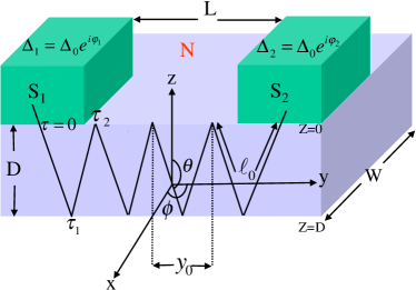
Figure 1: (Color online), Schematic of the SNS junction. The current flow between two superconductors (${\rm S_{1,2}}$) through a Normal layer (N). The NS interfaces are perfectly transparent.

In this section, we calculate the Josephson current for a clean SNS junction in the presence of an external magnetic field $\mathbf{H}$. The setup is schematically shown in Fig. 1. It consists of a normal metallic (N) layer of the thickness $D$ and width $W$ on which two superconducting electrodes are deposited in a distance of $L$. This planar Josephson structure was studied experimentally in Ref. KlapwijkNature2006, with a half metallic N layer. A phase difference $\varphi$ between order parameters of the superconductors drives a Josephson supercurrent through the parts of N layer underneath the superconductors and the junction N part ($-L/2\leq y\leq L/2$). The magnetic field $\mathbf{H}=-H\hat{\textrm{x}}$ is applied in the plane of N layer perpendicular to the direction of supercurrent flow. We consider a clean structure with all dimensions $L,W,D$ being smaller than the electronic impurity mean free path $\ell_{\rm imp}$ and ideally transparent NS-interfaces. At the same time, the Fermi wavelength is small compared to $L,W,D,$ and the superconducting coherence length $\xi_{0}=v_{\rm F}/2\Delta_{0}(T=0)$ (we use the system of units with $\hbar=k_{\text{B}}=1$). Under these conditions the electronic properties of the system can be derived from the Eilenberger equations for the semiclassical matrix Green’s function $\hat{\textit{g}}$,

$$-v_{\rm F}\mathbf{n}.\nabla\hat{\textit{g}}=\omega_{n}[\hat{\tau}_{3},\hat{\textit{g}}~{}]+[\hat{\Delta}(\textbf{r}),\hat{\textit{g}}~{}],$$ (2)

The matrix Green’s function

$$\hat{\textit{g}}=\left(\begin{array}[]{cc}\textit{g}_{\omega_{n}}&f_{\omega_{n}}\\ f^{\dagger}_{\omega_{n}}&-\textit{g}_{\omega_{n}}\end{array}\right),$$

where the normal g and anomalous $f$ Green’s functions depend on the Matsubara frequency $\omega_{n}=\pi T(2n+1)$, on the coordinate r, and the direction of motion n; $\hat{\tau}_{i}$ (i=1,2,3) denotes the Pauli matrices in the Nambu space, and the matrix

$${\hat{\Delta}(\textbf{r})}=\left(\begin{array}[]{cc}\begin{array}[]{c}0\end{array}&\begin{array}[]{c}\Delta(\textbf{r})\end{array}\\ \begin{array}[]{c}\Delta^{\ast}(\textbf{r})\end{array}&\begin{array}[]{c}0\end{array}\end{array}\right)$$

represents the superconducting order parameter $\Delta(\textbf{r})$. The matrix Green’s function $\hat{\textit{g}}_{\omega_{n}}$ satisfies the normalization condition,

$$\hat{\textit{g}}^{2}=1 \textit{g}_{\omega_{n}}^{2}+f_{\omega_{n}}f^{\dagger}_{\omega_{n}}=1,$$ , (7)

where $f^{\dagger}_{\omega_{n}}(\textbf{r},\mathbf{n})=f^{\ast}_{\omega_{n}}(\textbf{r},-\mathbf{n})$. In components, the Eilenberger equations have the form

$$-v_{\rm F}\mathbf{n}.\nabla\textit{g}_{\omega_{n}} = \Delta(\textbf{r})f^{\dagger}_{\omega_{n}}-\Delta^{\ast}(\textbf{r})f_{\omega_{n}},$$ (8)

$$-v_{\rm F}\mathbf{n}.\nabla f_{\omega_{n}} = 2\omega_{n}f_{\omega_{n}}-2\Delta(\textbf{r})\textit{g}_{\omega_{n}}.$$ (9)

We solve these equations along an electronic quasiclassical trajectory (shown in Fig. 1) which is parameterized by $-\infty\leq\tau\leq\infty$ ZareyanPRL2001 ; ZareyanPRB2002 . Assuming a weak external magnetic field we neglect its effect on the orbital motion of the quasiparticles. The magnetic field then will have only phase effect which we will include by introducing the gauge invariant phase as

$$\varphi=\varphi_{0}-\frac{2\pi}{\Phi_{0}}\int_{0}^{\ell}\mathbf{A}.\mathbf{n}d\tau,$$ (10)

where $\varphi_{0}$ is the phase difference between two superconductors in the absence of the magnetic field, the second part is the phase accumulated by the quasiparticle on the trajectory due to the magnetic field $\mathbf{H}=\nabla\times\mathbf{A}$, with $\ell$ being the length of the trajectory inside N-layer. The vector potential is taken to be $\mathbf{A}=-Hz\hat{\textrm{y}}$.

A typical trajectory consists of three parts: the part extended from bulk of ${\rm S_{1}}$ ($\tau=-\infty$) to a point at ${\rm NS_{1}}$-interface $\tau=0$, the part inside N layer ($0<\tau<\ell$) which extends from a point at ${\rm NS_{1}}$-interface to a point at ${\rm NS_{2}}$-interface and the last part which extends from the point $\tau=\ell$ to the bulk of ${\rm S_{2}}$ ($\tau=\infty)$. Our equations are supplemented by the boundary conditions which determine the values of Green’s functions in the bulk ${\rm S_{1}}$ and ${\rm S_{2}}$,

$$f_{\omega_{n}}(\tau=\mp\infty) = \frac{\Delta_{0}(T)\exp(i\varphi_{1,2})}{\Omega_{n}},$$ (11)

$$\textit{g}_{\omega_{n}}(\tau=\mp\infty) = \frac{\omega_{n}}{\Omega_{n}}\ ,$$ (12)

where $\Omega_{n}=\sqrt{\Delta_{0}^{2}+\omega_{n}^{2}}$, and $\Delta_{0}(T)$ is the temperature-dependent superconducting gap. We neglect the variation of the order parameter close to NS-interfaces inside the superconductors and approximate the order parameter by the step-function, $\Delta(\textbf{r})=\Delta_{0}e^{i\varphi_{1}}\theta(\tau)+\Delta_{0}e^{i\varphi_{2}}\theta(\tau-L)$. We can obtain the Green’s function $\textit{g}_{\omega_{n}}$ on a trajectory inside N that is constant. It depends only on the length of that trajectory $\ell$ and the phase difference $\varphi_{0}$, which is given by

$$\textit{g}_{\omega_{n}}=\tanh[\omega_{n}\ell/v_{\rm F}+i\varphi_{0}/2+\mbox{\rm arcsinh}\ (\omega_{n}/\Delta_{0})]\ .$$ (13)

Note that in the presence of the magnetic field, the phase difference $\varphi_{0}$ is replaced by $\varphi$ (see Eq. (10)).

The supercurrent density can then be obtained by averaging (13) over all different possible classical trajectories. This corresponds to an averaging over Fermi velocity directions. In the presence of the planar magnetic field, we find

$$\mathbf{j(\mathbf{r})}=e\mathcal{N}(0)Tv_{\rm F}\sum_{\omega_{n}}\int\mathbf{n}\mbox{\rm Im}\ \textit{g}_{\omega_{n}}(\ell,v_{\rm F})\sin\theta d\theta d\phi\ .$$ (14)

Here $\mathcal{N}(0)$ is the density of states at the Fermi surface and $\mbox{Im}\ \textit{g}_{\omega_{n}}(\ell,v_{\rm F})$ denotes the imaginary part of the normal component of the matrix Green’s function, given by

$$\mbox{Im}\ \textit{g}_{\omega_{n}} = \frac{\Delta_{0}^{2}(T)\sin\varphi}{(\Omega_{n}^{2}+\omega_{n}^{2})\cosh\chi+2\Omega_{n}\omega_{n}\sinh\chi+\Delta_{0}^{2}\cos\varphi},$$

$$\chi = \frac{\omega_{n}\ell}{\pi T_{c}\xi_{0}}.$$ (16)

To calculate the integral of the vector potential along the quasiclassical trajectories, we split it into the segments as shown in Fig. 1,

$$\int_{0}^{\ell}\mathbf{A}.\mathbf{n}d\tau=\int_{0}^{\tau_{1}}\mathbf{A}.\mathbf{n}d\tau+\int_{\tau_{1}}^{\tau_{2}}\mathbf{A}.\mathbf{n}d\tau+...$$

$$+\int_{\tau_{n-2}}^{\tau_{n-1}}\mathbf{A}.\mathbf{n}d\tau+\int_{\tau_{n-1}}^{\ell}\mathbf{A}.\mathbf{n}d\tau\ .$$ (17)

For the first term of the right side, we can write

$$\int_{0}^{\tau_{1}}\mathbf{A}.\mathbf{n}d\tau=-H\int_{0}^{y_{0}/2}zdy\ .$$

Since the equation for this segment of the trajectory is $z=D(1-y(D\tan\theta\sin\phi)^{-1}$, we get for the integral

$$\int_{0}^{\tau_{1}}\mathbf{A}.\mathbf{n}d\tau=-\frac{HDy_{0}}{4}\ ,y_{0}=2D\tan\theta\sin\phi\ .$$ (18)

where $y_{0}$ is shown in Fig. 1. Similarly, we find identical results for the integrals of the vector potential over the other segments. Therefore for a trajectory with the length $\ell$, the phase induced by the planar magnetic field proportional to

$$\Phi_{\ell}=\int_{0}^{\ell}\mathbf{A}.\mathbf{n}d\tau=\frac{-HDNy_{0}}{2}\ ,$$ (19)

where $N$ is the number of the triangles (each triangle consists of two segments) for the trajectory of the length $\ell$ passing through the point $z$, $N=[L/(4D\tan\theta\sin\phi)-z/(2D)]+[L/(4D\tan\theta\sin\phi)+z/(2D)]+2$, with the square brackets denoting the integer part.

Thus, for the phase difference, we obtain

$$\varphi = \varphi_{0}+\pi\frac{\Phi}{\Phi_{0}}\frac{2ND\tan\theta\sin\phi}{L}.$$

Here $\Phi=HDL$ is the total flux through the junction. Substituting this into Eq. (14) and taking the $y$-component of the current, we obtain the final expression

$$\frac{I(\varphi_{0})}{I_{0}} = \frac{T}{T_{c}\xi_{0}}\sum_{\omega_{n}=-\infty}^{\omega_{n}=\infty}\int_{0}^{D}\int_{0}^{\pi}\int_{-1}^{1}\frac{\Delta_{0}^{2}(T)\sin\left(\varphi_{0}+\pi\frac{\Phi}{\Phi_{0}}\frac{\ell}{L}(1-x^{2})^{1/2}\sin\phi\right)(1-x^{2})^{1/2}dx\sin\phi d\phi dz}{(\Omega_{n}^{2}+\omega_{n}^{2})\cosh\chi+2\Omega_{n}\omega_{n}\sinh\chi+\Delta_{0}^{2}\cos\left(\varphi_{0}+\pi\frac{\Phi}{\Phi_{0}}\frac{\ell}{L}(1-x^{2})^{1/2}\sin\phi\right)},$$

$$I_{c}(\Phi) = max_{{}_{{}_{0\leq\varphi_{0}\leq 2\pi}}}\frac{I(\varphi_{0})}{I_{0}},$$ (21)

with the notations $\cos\theta=x$ and $I_{0}=2ev_{\rm F}\mathcal{N}(0)T_{c}W\xi_{0}$, and $W$ being the width of the normal layer in the $x$-direction, which for a wide junction is taken to be much larger than $D$ and $L$. The length $\ell$ of the quasi-classical trajectory equals $\ell=2ND/x$. For low temperatures, $T\ll v_{F}/L$, the summation over Matsubara frequencies in Eq. (21) can be replaced by the integration,

$$2\pi T\sum(...)\rightarrow\int(...)d\omega\rightarrow\int(...)\Delta_{0}(T)\cosh\mu d\mu\ ,$$

where $\omega=\Delta_{0}\sinh\mu$. For a long SNS junction ($L\gg\xi_{0}$) and low temperature, Eq. (21) is simplified as

$$\frac{I(\varphi_{0})}{I_{0}}=\int_{0}^{D}\int_{0}^{\pi}\int_{-1}^{1}E(\varphi,\ell)(1-x^{2})^{1/2}dx\sin\phi d\phi dz,$$

$$E(\varphi,\ell)=\frac{2D}{\xi_{0}}\left(\frac{\xi_{0}}{\ell}-\frac{2\xi_{0}^{2}}{\ell^{2}}\right)\sum_{m=1}^{\infty}(-1)^{m}\frac{\sin(m\varphi)}{m},$$ (22)

where $E(\varphi,\ell)$ is the Fourier Series, given by (see Ref. GolubovRMP2004, )

$$E(\varphi,\ell)=\frac{D}{\xi_{0}}\left(\frac{\xi_{0}}{\ell}-\frac{2\xi_{0}^{2}}{\ell^{2}}\right)\bigg{(}\varphi-2\pi\left[\frac{\varphi}{2\pi}+\frac{1}{2}\right]\bigg{)}.$$ (23)

III Discussion and results

Equation (21) expresses the magnetic interference pattern $I_{c}(\Phi)$ of a ballistic SNS junction in the presence of an in-plane magnetic flux $\Phi$. In this section we analyze $I_{c}(\Phi)$ in terms of the length-to-thickness ratio $L/D$ and the temperature $T$ for $D/\xi_{0}={\rm 1/30}$.

Figure 2: The critical current dependence on the external magnetic field, applied in the plane of the normal metallic layer for different temperatures, $L/D={\rm 100}$ and $D/\xi_{0}={\rm 1/30}$ .

Let us start with analyzing the case of very large $L/D$. Figure 2 a,b shows oscillations of $I_{c}(\Phi)$ for $L/D={\rm 100}$ and at low ($T=0.1T_{c}$) and high ($T=0.95T_{c}$) temperatures, respectively. At low temperatures the the critical current goes through nonzero minima at finite fluxes. The amplitude of supercurrent minima decrease with $\Phi$ and drops to zero at $\Phi\gg\Phi_{0}$. Compared to an ordinary magnetic interference pattern, the oscillations are weakly damped since their amplitude decreases with $\Phi$ much slower than as $~{}1/\Phi$. With increasing temperature, the amplitude of the oscillations decreases. Also, the minimal values of the supercurrent decreases and vanishes as $T\rightarrow T_{c}$, where $\Delta_{0}(T)\ll T$. Note that at both low and high temperatures the period of oscillations varies from ${\rm 0.92}\Phi_{0}$ (first minima) at low magnetic fluxes to $\Phi_{0}$ at high fluxes. The result that the period of oscillations is temperature independent comes from the fact that the gauge invariant phase in the argument of the sine and cosine functions in Eq. (21) does not contain any temperature-dependent factors.

Figure 3: The same as Fig. 2 but for $L/D={\rm 10}$.

Figure 3 presents the magnetic interference pattern for a lower $L/D={\rm 10}$ and at the same temperatures as Figure 2. From these plots we see that lowering $L/D$ has two main effects. First, the rate at which the amplitude of $I_{c}$ oscillation decreases with $\Phi$ increases. Second, the period of oscillations at both low and high temperatures becomes smaller $\simeq{\rm 0.72}\Phi_{0}$ at small fluxes. Increasing $\Phi$ the period increases up to $\simeq\Phi_{0}$. Again as in Figs. 2 the value of supercurrent at the minima vanishes as the temperature approaches $T_{c}$.

Still lower period of oscillations at small fluxes can be reached at low values of $L/D$. This is illustrated in Fig. 4 where the magnetic interference pattern is presented for $L/D={\rm 5}$. Clearly the decay is close to the ordinary pattern (1), i.e. $~{}1/\Phi$, and the period can be as small as half the flux quantum.

The existence of the nonzero minima in the oscillations of $I_{c}(\Phi)$ is related to the non-sinusoidal phase dependence of the Josephson current (21) which is more pronounced at low temperatures $T\ll T_{c}$. We have found that $I_{c}(\Phi)$ undergoes a change of sign at a nonzero minimum. At such point the amplitude of the first harmonic ($\propto\sin{\varphi_{0}}$) of the Josephson current vanishes and $I_{c}(\Phi)$ is determined by the amplitude of the higher (mainly second) harmonics which change sign upon crossing the minimum. Similar effect was found before in ferromagnetic Josephson junctions (see Ref. SellierPRL2004, -RyazanovPRB2006, and references therein). As $T$ approaches $T_{c}$ the ratio $\Delta_{0}(T)/T$ goes to zero and the current-phase relation (Eq. (21)) becomes sinusoidal and consequently the nonzero minima disappear.

The dependence of the period of the oscillations on the magnetic flux and the geometry can be understood in terms of the difference between the magnetic flux $\Phi_{\ell}$ (Eq. (19)) enclosed by a trajectory of length $\ell$, and half of the flux $\Phi$ penetrating through the area $DL$. The difference comes from the fact that a trajectory which does not pass through the edges of S contacts has extra parts in N-layer which lie outside the area $DL$ (See Fig. 1). Writing $\Phi_{\ell}=\Phi/2+\delta\Phi_{\ell}$, the difference $\delta\Phi_{\ell}$ vanishes only for the trajectories which pass through the edges of S contacts. A finite averaged $\langle\delta\Phi_{\ell}\rangle$ over different trajectories means that the period of $I_{c}(\Phi)$-oscillations, obtained from Eq. (21), differs from $\Phi_{0}$. We note that in the limit of thin N-layer $L\gg D$ or high magnetic fluxes $\Phi\gg\Phi_{0}$ the contribution of the trajectories which are not passing through the edges is negligibly small in the interference structure and the period of the oscillation approaches $\Phi_{0}$ (See Figs. 2-4).

Figure 4: The same as Fig. 2 but for $L/D={\rm 5}$.

In contrast to $L\gg D$ case, for smaller $L/D$ the contribution of the trajectories not passing through the edges is important. Because of having larger length, a trajectory not passing through the edges has bigger contribution in gaining the effect of the magnetic flux as compared to the corresponding trajectory (having the same orientation $\theta$ and $\phi$) passing through the edges. Therefore we expect that the effect of magnetic flux is more pronounced for thicker N layers compare to the thinner ones, which explains why the decrease of the amplitude of $I_{c}(\Phi)$-oscillations with $\Phi$ is faster for smaller $L/D$.

IV Conclusions

In conclusion, we have studied Josephson effect in a SNS structure made of a thin ballistic N-layer of thickness $D$ on which two superconducting electrodes are deposited at the distance $L$ between each other. A magnetic field is applied in plane of the N-layer which modulates the superconducting interference and leads to a decaying oscillatory variation of the critical supercurrent $I_{c}(\Phi)$ with the magnetic flux $\Phi$. Using the quasiclassical Green’s functions approach, we have shown that such a magnetic interference pattern has three main differences with that of an ordinary pattern. First, at low temperatures the oscillations of the critical current $I_{c}(\Phi)$ go through the minima at which the supercurrent has nonzero values. Second, for a large $L/D$ the amplitude of the quasi-periodic oscillations of $I_{c}(\Phi)$ decays at a rate which is much slower than $1/\Phi$. Third, at low magnetic fluxes the oscillations can have a period smaller than the magnetic quantum flux $\Phi_{0}$ depending on $L/D$. These features have been experimentally observed recently KlapwijkNature2006 .

- (1) B. D. Josephson, Rev. Mod. Phys. 36, 216 (1964).
- (2) J. M. Rowell, Phys. Rev. Lett. 11, 200 (1963).
- (3) T. N. Antsygina, E. N. Bratus, and A. V. Svidzinskii, Fiz. Nizk. Temp. 1, 49 (1975) [ Sov. J. Low Temp. Phys. 1, 23 (1975)].
- (4) J. P Heida, B. J. van Wees, T. M. Klapwijk, and G. Borghs, Phys. Rev. B 57, 5618(R) (1998).
- (5) V. Barzykin and A. M. Zagoskin, cond-matt/9805104 (unpublished).
- (6) U. Ledermann, A. L. Fauchère, and G. Blatter, Phys. Rev. B 59, 9027(R) (1999).
- (7) R. S. Keizer, S. T. B. Goennenwein, T. M. Klapwijk, G. Miao, G. Xiao, and A. Gupta, Nature 439, 825 (2006).
- (8) F. S. Bergeret, A. F. Volkov, and K. B. Efetov, Rev. Mod. Phys. 77, 1321 (2005).
- (9) F. S. Bergeret, A. F. Volkov, and K. B. Efetov, Phys. Rev. Lett. 86, 4096 (2001).
- (10) M. Zareyan, W. Belzig, and Yu. V. Nazarov, Phys. Rev. Lett. 86, 308 (2001).
- (11) M. Zareyan, W. Belzig, and Yu. V. Nazarov, Phys. Rev. B. 65, 184505 (2002).
- (12) A. G. Golubov, M. Yu. Kupriyanov, and E. llíchev, Rev. Mod. Phys. 76, 411 (2004); C. Ishii, Prog. Theor. Phys. 44, 1525 (1970).
- (13) H. Sellier, C. Baraduc, F. Lefloch, and R. Calemczuk, Phys. Rev. Lett. 92, 257005 (2004).
- (14) R. Mélin, Europhys. Lett., 69, 121 (2005).
- (15) M. Houzet, V. Vinokur, and F. Pistolesi, Phys. Rev. B 72, 220506(R) (2005).
- (16) A. Buzdin, Phys. Rev. B 72, 100501(R) (2005).
- (17) G. Mohammadkhani and M. Zareyan, Phys. Rev. B. 73, 134503 (2006); V. Braude and Ya. M. Blanter, arXiv:0706.1746.
- (18) S. M. Frolov, D. J. Van Harlingen, V. V. Bolginov, V. A. Oboznov, and V. V. Ryazanov, Phys. Rev. B 74, 020503 (2006).