Optimized norm-conserving Hartree-Fock pseudopotentials for plane-wave calculations

Abstract

We report Hartree-Fock (HF) based pseudopotentials suitable for plane-wave calculations. Unlike typical effective core potentials, the present pseudopotentials are finite at the origin and exhibit rapid convergence in a plane-wave basis; the optimized pseudopotential method [A. M. Rappe et al. , Phys. Rev. B 41 1227–30 (1990)] improves plane-wave convergence. Norm-conserving HF pseudopotentials are found to develop long-range non-Coulombic behavior which does not decay faster than $1/r$, and is non-local. This behavior, which stems from the nonlocality of the exchange potential, is remedied using a recently developed self-consistent procedure [J. R. Trail and R. J. Needs, J. Chem. Phys. 122, 014112 (2005)]. The resulting pseudopotentials slightly violate the norm conservation of the core charge. We calculated several atomic properties using these pseudopotentials, and the results are in good agreement with all-electron HF values. The dissociation energies, equilibrium bond lengths, and frequency of vibrations of several dimers obtained with these HF pseudopotentials and plane waves are also in good agreement with all-electron results.

I Introduction

In nearly all plane-wave density functional calculations kohn_nobel , the use of pseudopotentials is essential in order to eliminate the atomic core states and the strong potentials that bind them. This results in replacing the electron-nuclear Coulomb interaction by a weaker (often angular-momentum dependent) potential. The advantage is the reduced computational cost, due to reduction in the number of electrons and in the plane-wave basis cutoff pickett .

In the physics community, pseudopotentials are typically constructed using density functional theory (DFT) due to its success in electronic structure calculations BHS ; RRKJ ; TM . Pseudopotentials based on methods other than DFT are less widely available. One of the key ingredients of most of these pseudopotentials is their “softness,” meaning that they provide rapid convergence in a plane-wave basis. On the other hand, in the chemistry community, Hartree-Fock (HF) pseudopotentials or effective core potentials (ECPs) are mostly used dolg_rev ; SBKJC ; hay_wadt_psp ; CLP_psp ; dolg_psp . Most of the available ECPs, which are typically expressed in a Gaussian basis, are of limited use in plane-wave calculations, mainly because of their singular behavior at the origin and slow convergence in a plane-wave basis.

Recently, there has been a growing interest in developing soft-core HF pseudopotentials greeff_lester ; lester_psp ; trail_needs1 ; trail_needs2 . HF pseudopotentials have been applied in diffusion Monte Carlo calculations, and the results suggest that they are better suited for correlated calculations than DFT-based pseudopotentials greeff_lester . In addition, HF pseudopotentials could be useful in certain calculations where a negatively charged reference state is needed; HF tends to bind electrons more strongly than DFT. Also, hybrid exchange-correlation functionals, which include some proportion of HF exact exchange (notably B3LYP B3LYP ) have proved successful in electronic structure calculations, and whether HF or B3LYP based pseudopotentials would be useful in these type of calculations remains to be explored.

Trail and Needs trail_needs1 have recently found that norm-conserving HF pseudopotentials constructed using standard norm-conserving pseudopotential methods develop a non-decaying and non-local tail. These pseudopotentials would generally lead to erroneous results, and even infinite energies in solid state calculations. Previously, pseudopotentials based on exact exchange within the optimized potential method (OPM) were also found to develop a similar, but local and eventually decaying long range structure bk_exact_xc ; stadele_exact_xc ; engel_exact_xc , which led to erroneous results in applications.

Different schemes have been proposed to cure the long-range behavior in the HF and OPM type pseudopotentials mentioned above. Originally with the OPM method, different groups developed procedures for reducing or eliminating the unphysical long-range behavior, while retaining desired eigenvalue matching and norm conservation of the pseudopotential bk_exact_xc ; stadele_exact_xc . This procedure was later implemented in a self-consistent manner by altering the pseudo-orbitals over all space, which led to a small violation of the norm conservation of the core charge. Nevertheless, the pseudopotentials proved transferable in both atomic and solid-state calculations engel_exact_xc . Trail and Needs fixed the long-range unphysical behavior using a similar self-consistent approach trail_needs1 that also slightly violates norm conservation. Ovcharenko et al. lester_psp have recently developed HF-based pseudopotentials which are finite at the origin and are expressed in terms of Gaussian basis, but are still relatively hard for typical plane-wave calculations, as we show in Sec. IV.

In this paper, we construct soft-core HF based pseudopotentials following the Rappe-Rabe-Kaxiras-Joannopoulos (RRKJ) method RRKJ . We use a self-consistent approach to restore the Coulombic tail in a manner similar to that used by Trail and Needs trail_needs1 ; casino_psp . Pseudopotentials are highly non-unique entities, and it is useful to have several alternative forms available with different properties. For example, one of the advantages of the RRKJ construction scheme is the softness of the resulting pseudopotentials.

The rest of the paper is organized as follows. We first review the general construction scheme of the RRKJ pseudopotentials, and the procedure we used to “localize” the pseudopotentials (remove the long tail behavior). The crucial steps in the validation of the pseudopotentials are the study of their convergence and transferability, i. e. how well the pseudopotentials converge in a plane-wave basis set, and how well they perform in environments different than the reference configuration. These steps are explored in Sections III and IV. In Sec. III, we study plane-wave convergence of the atoms, and we investigate the transferability by looking at the ionization energy, electron affinity, and excitation energy of the first- and second-row elements. In Sec. IV, we study several dimers at the HF level, and compare both the all-electron and pseudopotential results. Finally, in Sec. V, we conclude by summarizing the main points.

II Pseudopotential construction

We follow the usual density functional theory approach for the construction of the norm-conserving pseudopotentials starting from an all-electron (AE) atomic calculation pickett . However, in this case, we solve the Hartree-Fock instead of the Kohn-Sham equations. Our HF solver is adapted from the code of Ref. f_fisher, .

The pseudopotential construction starts by choosing an electronic reference state, and then solving the Schrödinger equation of the system for the eigenstates $\Phi_{nl}({\bf r})$ and eigenvalues $\epsilon_{nl}$. The wavefunction can be written as $\Phi_{nl}({\bf r})=\phi_{nl}(r)Y_{lm}(\theta,\phi)/r$ where $Y_{lm}(\theta,\phi)$ are the spherical harmonics. The orbitals $\phi_{nl}(r)$ satisfy the radial Schrödinger equation:

$${\left[\hat{T}+\hat{V}_{\mathrm{ion}}+\hat{V}_{\mathrm{HF}}[\{\phi(r)\}]\right]}\phi_{nl}(r)=\epsilon_{nl}\phi_{nl}(r),$$ (1)

where $\hat{T}=-d^{2}/(2dr^{2})+l(l+1)/(2r^{2})$, $\hat{V}_{\mathrm{ion}}(r)=-{Z}/{r}$ is the bare nuclear potential, and $Z$ is the atomic number. $\hat{V}_{\mathrm{HF}}[\{\phi(r)\}]$ is the HF potential defined such that,

$$\hat{V}_{\rm{HF}}[\{\phi(r)\}]\phi_{nl}({r})=\hat{V}_{H}[\{\phi(r)\}]\phi_{nl}({r})+\hat{V}_{x}^{nl}[\{\phi(r)\}]\phi_{nl}({r});$$ (2)

$$\hat{V}_{H}[\{\phi(r)\}]=\sum_{nl}\int d{\bf r^{\prime}}\,\frac{|\Phi_{nl}({\bf{r^{\prime}}})|^{2}}{|{\bf r}-\bf{r^{\prime}}|};$$ (3)

$$\hat{V}_{x}^{nl}[\{\phi(r)\}]\Phi_{nl}({\bf r})=\sum_{n^{\prime}l^{\prime}}\int d{\bf r^{\prime}}\,\frac{\Phi_{nl}({\bf r^{\prime}})\Phi_{n^{\prime}l^{\prime}}^{*}({\bf{r^{\prime}})}}{|{\bf r}-\bf{r^{\prime}}|}\Phi_{n^{\prime}l^{\prime}}({\bf{r}}).$$ (4)

For convenience, equal and opposite self interaction terms are included in both the Hartree and exchange terms. Therefore, the Hartree potential $\hat{V}_{H}[\{\phi(r)\}]\equiv\hat{V}_{H}[\rho(r)]$ is a functional of the spherically averaged total electronic density $\rho(r)=\sum_{nl}|\phi_{nl}(r)|^{2}$.

The second step in the construction of norm-conserving pseudopotentials typically begins with the generation of a smooth set of pseudo-orbitals $\tilde{\phi}_{nl}(r)$ to replace the AE orbitals $\phi_{nl}(r)$, such that $\tilde{\phi}_{nl}(r)$ equals the all-electron orbital beyond some cutoff distance $r_{c}$. Different norm-conserving pseudopotentials mainly differ in the form of $\tilde{\phi}_{nl}(r)$ for $r<r_{c}$, and the guiding principles used to construct $\tilde{\phi}_{nl}(r)$.

In the RRKJ method, the pseudo-orbitals in the core region are expressed as a linear combination of spherical Bessel functions $j_{l}(q_{k}r)$

$$\tilde{\phi}_{nl}(r)=\left\{\begin{aligned} \sum_{k=1}^{N_{b}}c_{nlk}\,\,rj_{l}(q_{k}r)&&r<r_{c}\\ \phi_{nl}(r)&&r\geq r_{c}.\end{aligned}\right.$$ (5)

The Bessel wave-vectors $q_{k}$ are chosen such that,

$$\frac{j_{l}^{{}^{\prime}}(q_{k}r_{c})}{j_{l}(q_{k}r_{c})}=\frac{\phi_{nl}^{{}^{\prime}}(r_{c})}{\phi_{nl}(r_{c})}\;\;\;\;\;\;\;\;\;k=1,\ldots,N_{b}$$ (6)

where $j_{l}^{{}^{\prime}}(q_{k}r)$ and $\phi_{nl}^{{}^{\prime}}(r)$ are the derivatives of $j_{l}(q_{k}r)$ and $\phi_{nl}(r)$ with respect to $r$, respectively. $N_{b}$ is the number of Bessel coefficients, $c_{nlk}$.

The key ingredient of the RRKJ method is the optimization of the Bessel coefficients, $c_{nlk}$, to minimize the residual kinetic energy defined as follows:

$$\Delta T_{nl}(\{c_{nlk}\},q_{c})=-\int_{0}^{\infty}d{\bf r}\,\tilde{\Phi}_{nl}({\bf r})\nabla^{2}\tilde{\Phi}_{nl}({\bf r})$$ (7)

$$-\int_{0}^{q_{c}}d{\bf q}\,{\bf q}^{2}|\tilde{\Phi}_{nl}({\bf q})|^{2},$$

where $\tilde{\Phi}_{nl}({\bf q})$ is the Fourier transform of real space pseudo-orbital $\tilde{\Phi}_{nl}({\bf r})=\tilde{\phi}_{nl}(r)Y_{lm}(\theta,\phi)/r$, and $q_{c}$ is the target wavevector above which the contribution to the residual kinetic energy is as small as possible. For a particular $q_{c}$, the planewave energy cutoff required to achieve total energy convergence of $\Delta T_{nl}$ is given by the square of the maximum value of $q_{c}$ over all orbitals RRKJ .

The optimization of $\Delta T_{nl}(\{c_{nlk}\},q_{c})$ is constrained to pseudo-orbitals that are continuous at $r_{c}$, with continuous first and second derivatives [in fact, one of these local constraints would be already satisfied due to Eq.(6)], and that satisfy norm conservation of the core charge:

$$\int_{0}^{r_{c}}dr\,|\tilde{\phi}_{nl}(r)|^{2}=\int_{0}^{r_{c}}dr\,|\phi_{nl}(r)|^{2}.$$ (8)

This procedure defines all the Bessel coefficients in Eq. (5), and $N_{b}$ must be at least 3 to allow the constraints to be satisfied. Any additional parameters will be optimized by minimizing the residual kinetic energy due to the non-linearity of Eq. (7). Throughout this study, we used $N_{b}=6$.

The screened pseudopotential ${\hat{V}}_{\mathrm{scr}}^{nl}(r)$ is defined as the potential that makes the desired pseudo-orbital $\tilde{\phi}_{nl}(r)$ an eigenstate of the one-electron Schrödinger equation, with the same eigenvalue $\epsilon_{nl}$ as the corresponding all-electron state:

$$\left[\hat{T}+{\hat{V}}_{\mathrm{scr}}^{nl}(r)\right]\tilde{\phi}_{nl}(r)=\epsilon_{nl}\,\tilde{\phi}_{nl}(r).$$ (9)

This equation can now be inverted, thanks to the nodeless character of $\tilde{\phi}_{nl}(r)$, to obtain the screened pseudopotential:

$${{\hat{V}}_{\mathrm{scr}}}^{nl}(r)=\epsilon_{nl}(r)-\frac{\ell(\ell+1)}{2\,r^{2}}+\frac{1}{2{\tilde{\phi}_{nl}(r)}}\frac{d^{2}}{dr^{2}}\left[\tilde{\phi}_{nl}(r)\right].$$ (10)

Note that ${\hat{V}}_{\mathrm{scr}}^{nl}(r)$ is a continuous function because of the continuity requirements imposed on the pseudo-orbital $\tilde{\phi}_{nl}(r)$ and its first two derivatives.

The last step in the construction of pseudopotentials is to remove the screening effects of the valence electrons, and to obtain the ionic pseudopotential. This is done by subtracting the Hartree and exchange-potential contributions of the valence electrons from the screened potential ${{\hat{V}}}_{\mathrm{scr}}^{nl}(r)$. That is,

$${{\hat{V}}}_{\mathrm{ion}}^{nl}(r)={{\hat{V}}}_{\mathrm{scr}}^{nl}(r)-\hat{V}_{H}[\{\tilde{\phi}(r)\}_{v}]-\frac{\hat{V}_{{x}}^{nl}[\{\tilde{\phi}(r)\}_{v}]\tilde{\phi}_{nl}(r)}{\tilde{\phi}_{nl}(r)},$$ (11)

where $\{\tilde{\phi}(r)\}_{v}$ includes only the valence orbitals. Note that the last term in Eq. (11), the exchange potential, is orbital dependent, and its explicit construction is feasible because the pseudo-orbitals are nodeless.

Up to this point, the pseudopotential construction recipe mirrors exactly the procedure done in regular norm-conserving pseudopotentials based on DFT, except that the original Hamiltonian is the HF and not the KS Hamiltonian. However, the resulting ionic potentials, ${{\hat{V}}}_{\mathrm{ion}}^{nl}(r)$, have different behavior for large $r$, which in turn stems from the corresponding large-$r$ behavior of the HF and KS orbitals. It was shown by Handeler et al. handler_limits_hf that the HF orbitals decay at infinity as

$$\phi_{nl}(r)=r^{\beta_{nl}+1}e^{-\alpha r}\left[a_{nl}+\frac{b_{nl}}{r}+{\cal{O}}(1/r^{2})\right],$$ (12)

where $\alpha=(-2\epsilon_{\mathrm{HO}})^{1/2}$ is determined by the eigenvalue of the highest occupied orbitals $\epsilon_{\mathrm{HO}}$, and $\beta_{nl}$ is an orbital dependent quantity handler_limits_hf . This behavior is to be contrasted with the exponential decaying behavior of the KS orbitals, $\phi_{nl}(r)\propto\exp[(-2\epsilon_{nl})^{1/2}r]$ for large $r$.

In DFT-based pseudopotentials, the exchange potential is replaced by the exchange-correlation functional of the electron density $\rho(r)$, which decays exponentially to zero for large $r$. Thus, the ionic potential ${{\hat{V}}}_{\mathrm{ion}}^{nl}(r)=-Z_{v}/r$ for large $r$ where $Z_{v}$ is the valence charge density.

The effect of the special long-range behavior of the HF orbitals on the ionic pseudopotential ${{\hat{V}}}_{\mathrm{ion}}^{nl}(r)$ can be understood by writing ${\hat{V}}_{\mathrm{ion}}^{nl}(r)$ as,

$${\hat{V}}_{\mathrm{ion}}^{nl}(r)=-\frac{Z}{r}+\hat{V}_{H}[\rho-\tilde{\rho_{v}}]+\frac{\hat{V}_{{x}}^{nl}[\{{\phi}(r)\}]{\phi}_{nl}(r)}{{\phi}_{nl}(r)}$$ (13)

$$-\frac{\hat{V}_{{x}}^{nl}[\{\tilde{\phi}(r)\}_{v}]\tilde{\phi}_{nl}(r)}{\tilde{\phi}_{nl}(r)}\,\,\,\,\,{\rm for\,\,\,}r>r_{c},$$

where the Schrödinger equation of Eq. (1) is used. Here $\rho(r)$ is the total electronic charge density while $\tilde{\rho}_{v}(r)$ is the pseudo-valence charge density. In the HF case, the exchange potential is a non-local functional of the HF orbitals as shown in Eq. (4). In particular, the leading behavior of the numerator for large $r$ will be $r^{\beta}e^{-\alpha r}$ where $\beta=\max_{nl}\beta_{nl}$, while the denominator will go as $r^{\beta_{nl}+1}e^{-\alpha r}$. Therefore, the exchange potential, as computed in Eq. (13), is not guaranteed to decay faster than $1/r$. In fact, the exchange potential can even grow without bound for large $r$ when computed in this way. This is the source of the non-local long-range non-Coulombic tail in the HF pseudopotentials trail_needs1 .

Table 1: A summary of the cutoff radii (in atomic units) for the pseudopotentials for $s$, $p$, and $d$ channels used in the atomic calculations. The last column shows $q_{c}^{\rm{max}}$, the largest $q_{c}$ value over all the orbitals (in Ry^1/2). The cutoff energy for a planewave basis is approximately the square of $q_{c}^{\rm{max}}$.

Atom	$r_{cs}$	$r_{cp}$	$r_{cd}$	$q_{c}^{\rm{max}}$
H	0.50	0.50	0.50	10.8
He	0.60	0.60	0.60	12.8
Li	2.19	2.37	2.37	2.7
Be	1.41	1.41	1.41	6.2
B	1.88	1.96	1.96	4.0
C	1.10	1.10	1.10	8.3
N	0.94	0.88	0.84	10.6
O	0.80	0.75	0.99	12.6
F	0.70	0.64	0.89	15.0
Ne	0.63	0.57	0.63	17.1
Na	2.70	2.85	2.85	2.5
Mg	2.38	2.38	2.38	3.2
Al	1.94	2.28	2.28	3.9
Si	1.67	2.01	2.06	4.6
P	1.48	1.71	1.71	5.8
S	1.33	1.50	1.50	5.8
Cl	1.19	1.34	1.34	6.5
Ar	1.09	1.20	1.31	7.3

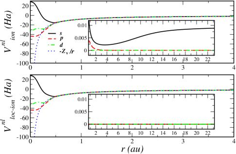
Figure 1: (Color online) The upper panel shows the Ne potential $V_{\rm{ion}}^{nl}$ constructed using the RRKJ method before the tail correction. The inset shows $\Delta V_{\rm{ion}}=V_{\rm{ion}}^{nl}+Z_{v}/r$ which displays the non-physical tail of the $s$-potential channel for large $r$. The lower panel shows $V_{\rm{loc-ion}}^{nl}$ after the tail correction procedure. In the inset, we show the large-$r$ behavior of $\Delta V_{\rm{loc-ion}}=V_{\rm{loc-ion}}^{nl}+Z_{v}/{r}$.

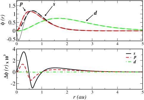
Figure 2: (Color online) The upper panel shows the all-electron (solid lines) and the localized pseudo-orbitals (dashed lines) of Ne constructed using the RRKJ method. The lower panel shows the difference in the pseudo-orbitals before and after the localization procedure (scaled by 10^-3).

In this work we follow the Trail and Needs self-consistent approach to localize the ionic pseudopotential trail_needs1 . The localized ionic potential ${\hat{V}}^{nl}_{{\rm{loc-ion}}}(r)$, which is forced to behave as $-Z_{v}/r$ for large $r$, is defined as

$${\hat{V}}^{nl}_{{\rm{loc-ion}}}(r)=\left\{\begin{array}[]{ll}\gamma_{nl}(r)+\hat{V}^{nl}_{{\rm{\mathrm{ion}}}}(r)&r<r_{\mathrm{loc}}\\ \\ \\ e^{-\xi(r-r_{\mathrm{loc}})^{2}}[\gamma_{nl}(r)+\hat{V}^{nl}_{{\rm{\mathrm{ion}}}}(r)+\\ \\ Z/r-\hat{V}_{\rm{H}}(\rho_{\rm{c}})]+\hat{V}_{\rm{H}}(\rho_{\rm{c}})-Z/{r}&r\geq r_{\mathrm{loc}}\end{array}\right.$$ (14)

where $\rho_{\rm{c}}(r)$ is the core charge density, $1/\sqrt{\xi}=r_{\rm{loc}}/16$ is the characteristic distance for the localized ${\hat{V}}^{nl}_{{\rm{loc-ion}}}(r)$ to approach $-Z_{v}/r$, and $r_{\mathrm{loc}}$ is the localization radius. For all pseudopotentials, the value of $r_{\mathrm{loc}}$ for each $l$-channel is fixed to be the same as the corresponding $r_{c}$. $\gamma_{nl}(r)$ is defined as $p_{nl}+q_{nl}f(r,r_{\mathrm{loc}})$ where $p_{nl}$ and $q_{nl}$ are parameters which are chosen to localize the ionic pseudopotential ${{\hat{V}}}_{\mathrm{ion}}^{nl}(r)$ in a self-consistent manner, and $f(r,r_{\mathrm{loc}})$ is a polynomial function whose explicit form depends on the pseudopotential construction method (see below).

The self-consistent procedure is performed as follows. First, starting with an initial guess for the $p_{nl}$ and $q_{nl}$ parameters, the HF equations with a new ionic potential, as defined in Eq. (14), are solved for a new set of orbitals and eigenvalues. The $p_{nl}$ and $q_{nl}$ parameters are then adjusted to minimize the error in the eigenvalues and logarithmic derivativeslogdernote1 . The procedure is then repeated until $p_{nl}$ and $q_{nl}$ parameters are found that give eigenvalues and logarithmic derivatives that closely match the all-electron values to the desired tolerance.

Finally, we define $f(r,r_{\mathrm{loc}})$ used in $\gamma_{nl}(r)$. For the case of Troullier-Martins pseudopotentials, we chose the same form as was used in Ref. trail_needs1 , namely $f(r,r_{\rm{loc}})=r^{4}\left(1-{2\,r^{2}}/{3r_{\mathrm{loc}}^{2}}\right)$ for $r<r_{\rm{loc}}$, and $f(r,r_{\rm{loc}})=r_{\mathrm{loc}}^{4}/{3}$ otherwise. For RRKJ pseudopotentials, we investigated a few different forms and found the results to be insensitive to the choices. We will report our results using $f(r,r_{\rm{loc}})=1-r/2r_{\mathrm{loc}}$ for $r<r_{\rm{loc}}$, and $f(r,r_{\rm{loc}})={r_{\mathrm{loc}}}/{2}$ for $r\geq r_{\rm{loc}}$.

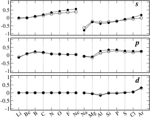
Figure 3: Amount of the violation of the core norm-conservation for the $s$, $p$, and $d$ pseudo-orbitals (in units of $10^{-3}$ electrons), respectively. There is less than $0.001$ electron shift between the valence and core regions. Pseudopotentials are constructed using the RRKJ (open circles), and TM (closed circles) methods.

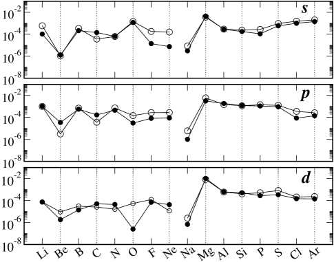
Figure 4: Similar to Fig. 3, except that we show the relative error in the logarithmic derivative at $r_{c}$ from the all-electron values. The relative error is defined as $|{1-L_{loc}}/{L}|$, where $L$ and $L_{loc}$ are the logarithmic derivative before and after the localization procedure is applied, respectively. The logarithmic derivative is approximately conserved in the localization procedure.

Table 2: Ionization energy study of the first- and second-row elements. The first column shows the all-electron ionization energy, while the other columns show the deviation from the AE result. Columns 2 and 3 show the pseudopotential ionization energies as obtained using the original and the localized RRKJ pseudopotentials [Eqs. (13) and (14), respectively]. Columns 4 and 5 show the same values as obtained using the TM method. For comparison, we show also the values obtained by Trail and Needs trail_needs1 . The pseudopotential parameters are summarized in Table 1. We show also the average abs. error for each pseudopotential with respect to the AE values. All energies are in Hartrees.

	AE	This work/RRKJ			This work/TM			TM
Atom	$E_{\rm ion}$	$\Delta{E}_{{\rm ion}}$	$\Delta\tilde{E}_{{\rm ion}}$		$\Delta{E}_{{\rm ion}}$	$\Delta\tilde{E}_{{\rm ion}}$		$\Delta{E}_{{\rm ion}}$	$\Delta\tilde{E}_{{\rm ion}}$
H	0.5000	$0.0000$	$0.0000$		$0.0000$	$0.0000$		$0.0000$	$0.0000$
He	0.8617	$-0.0009$	$-0.0008$		$-0.0007$	$-0.0007$		$-0.0006$	$-0.0006$
Li	0.1963	$0.0000$	$0.0000$		$0.0000$	$0.0000$		$0.0000$	$0.0000$
Be	0.2956	$-0.0002$	$-0.0002$		$-0.0002$	$-0.0002$		$-0.0002$	$-0.0002$
B	0.2915	$-0.0006$	$-0.0006$		$-0.0005$	$-0.0005$		$-0.0005$	$-0.0005$
C	0.3964	$-0.0009$	$-0.0008$		$-0.0006$	$-0.0005$		$-0.0006$	$-0.0005$
N	0.5129	$-0.0009$	$-0.0008$		$-0.0006$	$-0.0005$		$-0.0006$	$-0.0006$
O	0.4368	$0.0001$	$0.0001$		$0.0001$	$0.0001$		$0.0001$	$0.0000$
F	0.5776	$-0.0004$	$-0.0003$		$-0.0003$	$-0.0002$		$-0.0003$	$-0.0003$
Ne	0.7293	$-0.0008$	$-0.0007$		$-0.0006$	$-0.0004$		$-0.0005$	$-0.0005$
Na	0.1819	$-0.0002$	$-0.0002$		$-0.0001$	$-0.0001$		$-0.0001$	$-0.0001$
Mg	0.2428	$-0.0002$	$-0.0002$		$-0.0002$	$-0.0002$		$-0.0002$	$-0.0002$
Al	0.2020	$-0.0003$	$-0.0003$		$-0.0002$	$-0.0002$		$-0.0002$	$-0.0002$
Si	0.2812	$-0.0005$	$-0.0005$		$-0.0005$	$-0.0004$		$-0.0005$	$-0.0005$
P	0.3690	$-0.0009$	$-0.0008$		$-0.0008$	$-0.0008$		$-0.0008$	$-0.0008$
S	0.3317	$0.0011$	$0.0011$		$0.0012$	$0.0012$		$0.0011$	$0.0011$
Cl	0.4335	$-0.0003$	$-0.0002$		$0.0000$	$0.0000$		$-0.0002$	$-0.0002$
Ar	0.5430	$-0.0015$	$-0.0014$		$-0.0015$	$-0.0014$		$-0.0015$	$-0.0014$
Average abs. error		$0.0005$	$0.0005$		$0.0004$	$0.0004$		$0.0005$	$0.0004$
Maximum abs. error		$0.0015$	$0.0014$		$0.0015$	$0.0014$		$0.0015$	$0.0014$

Table 3: Similar to Table 2, except we show the electron affinity of the first- and second-row elements.

	AE	RRKJ			TM
Atom	$E_{\rm EA}$	$\Delta{E}_{{\rm EA}}$	$\Delta\tilde{E}_{{\rm EA}}$		$\Delta{E}_{{\rm EA}}$	$\Delta\tilde{E}_{{\rm EA}}$
B	$-0.0098$	$0.0001$	$0.0002$		$0.0$	$0.0001$
C	$0.0202$	$0.0002$	$0.0004$		$0.0001$	$0.0002$
N	$-0.0790$	$-0.0004$	$-0.0001$		$-0.0003$	$0.0000$
O	$-0.0196$	$0.0000$	$0.0003$		$-0.0001$	$0.0002$
F	$0.0501$	$0.0002$	$0.0006$		$0.0001$	$0.0004$
Al	$0.0016$	$0.0002$	$0.0002$		$0.0002$	$0.0002$
Si	$0.0353$	$0.0005$	$0.0005$		$0.0005$	$0.0005$
P	$-0.0199$	$-0.0009$	$-0.0007$		$-0.0008$	$-0.0007$
S	$0.0335$	$0.0001$	$0.0002$		$0.0000$	$0.0002$
Cl	$0.0948$	$0.0011$	$0.0013$		$0.0010$	$0.0011$
Average abs. error		$0.0004$	$0.0004$		$0.0003$	$0.0004$
Maximum abs. error		$0.0011$	$0.0013$		$0.0010$	$0.0011$

To illustrate the pseudopotential localization procedure, we show in the upper panel of Fig. 1 the pseudopotentials ${\hat{V}}^{nl}_{{\rm{ion}}}(r)$ of Ne as constructed using the RRKJ method with the parameters given in Table I. In the lower panel, we show the same Ne pseudopotentials after the self-consistent localization procedure. As can be seen, the differences between the upper and lower panels are rather small, and are in the core as well as in the valence regions. Most of the changes are within the core region, however. The insets show the long-range behavior of ${\hat{V}}^{nl}_{{\rm{ion}}}(r)+Z_{v}/r$. Note, in particular, in the upper panel, the non-decaying tail of the $s$-potential, which can be shown trail_needs1 to behave as $a+b/r$ for large $r$ where $a$ and $b$ are real numbers.

In Fig. 2, we show in the upper panel the all-electron and pseudo-orbitals after the localization procedure. The lower panel shows the difference in the pseudo-orbitals before and after the localization procedure. Again, changes are found in both the core and valence regions. One obvious drawback of the localization procedure is that the core-norm will be different from the all-electron value, i.e. Eq. (8) will be violated slightly. This can be seen in Fig. 2 because the changes in the orbitals for $r<r_{c}$ are all positive, and will integrate to a non-zero value.

As mentioned before, the localization procedure conserves the all-electron eigenvalues, and the logarithmic derivative. In practice, the logarithmic derivative is only conserved approximately. Figures 3 and 4 show a systematic study of the violations of the norm-conservation and the change in the logarithmic derivative at $r_{c}$ due to the localization procedure for the first- and second-row elements. The study was done using both the RRKJ and TM pseudopotentials. From Fig. 3, we see that there is less than $\approx 0.001$ electron shift between the core and the valence. The relative error between the logarithmic derivatives before and after applying the localization procedure is shown in Fig. 4 logdernote2 . As can be seen from both figures, both pseudopotential construction methods yield similar results.

Table 4: Excitation energy study of the first- and second-row elements. The first column shows the ground state configuration, and the second column shows the configuration of the excited states. The all-electron excitation energy is shown in the third column. The other columns show the deviation from the AE result, similar to Table 2. All energies are in Hartrees.

Atom		AE	RRKJ			TM			TM
Ground state	Excited state	$E_{{\rm exc}}$	$\Delta{E}_{{\rm exc}}$	$\Delta\tilde{E}_{{\rm exc}}$		$\Delta{E}_{{\rm exc}}$	$\Delta\tilde{E}_{{\rm exc}}$		$\Delta{E}_{{\rm exc}}$	$\Delta\tilde{E}_{{\rm exc}}$
H $1s^{1}[^{2}S]$	$2p^{1}[^{2}P]$	0.3750	$0.0000$	$0.0000$		$0.0000$	$0.0000$		$0.0000$	$0.0000$
	$3d^{1}[^{2}D]$	0.4444	$0.0000$	$0.0000$		$0.0000$	$0.0000$		$0.0000$	$0.0000$
He $1s^{2}[^{1}S]$	$1s^{1}2p^{1}[^{3}P]$	0.7302	$-0.0008$	$-0.0008$		$-0.0006$	$-0.0006$		$-0.0006$	$-0.0006$
	$1s^{1}3d^{1}[^{3}D]$	0.8061	$-0.0009$	$-0.0008$		$-0.0007$	$-0.0007$		$-0.0006$	$-0.0006$
Li $2s^{1}[^{2}S]$	$2p^{1}[^{2}P]$	0.0677	$0.0000$	$0.0000$		$0.0000$	$0.0000$		$0.0000$	$0.0000$
	$3d^{1}[^{2}D]$	0.1408	$0.0000$	$0.0000$		$0.0000$	$0.0000$		$0.0000$	$0.0000$
Be $2s^{2}[^{1}S]$	$2s^{1}2p^{1}[^{3}P]$	0.0615	$0.0011$	$0.0011$		$0.0010$	$0.0010$		$0.0020$	$0.0020$
	$2s^{1}3d^{1}[^{3}D]$	0.2389	$-0.0002$	$-0.0002$		$-0.0002$	$-0.0002$		$-0.0001$	$-0.0001$
B $2s^{2}2p^{1}[^{2}P]$	$2s^{1}2p^{2}[^{4}P]$	0.0784	$0.0023$	$0.0022$		$0.0020$	$0.0019$		$0.0020$	$0.0019$
	$2s^{2}3d^{1}[^{2}D]$	0.2353	$-0.0006$	$-0.0006$		$-0.0005$	$-0.0005$		$-0.0005$	$-0.0005$
C $2s^{2}2p^{2}[^{3}P]$	$2s^{1}2p^{3}[^{5}S]$	0.0894	$0.0060$	$0.0058$		$0.0054$	$0.0053$		$0.0054$	$0.0053$
	$2s^{2}2p^{1}3d^{1}[^{3}F]$	0.3402	$-0.0008$	$-0.0008$		$-0.0006$	$-0.0005$		$-0.0006$	$-0.0005$
N $2s^{2}2p^{3}[^{4}S]$	$2s^{1}2p^{4}[^{4}P]$	0.4127	$0.0029$	$0.0030$		$0.0030$	$0.0030$		$0.0031$	$0.0031$
	$2s^{2}2p^{2}3d^{1}[^{4}F]$	0.4565	$-0.0009$	$-0.0008$		$-0.0006$	$-0.0006$		$-0.0005$	$-0.0005$
O $2s^{2}2p^{4}[^{3}P]$	$2s^{2}2p^{3}3d^{1}[^{5}D]$	0.3809	$0.0001$	$0.0001$		$0.0001$	$0.0001$		$0.0000$	$0.0000$
	$2s^{1}2p^{5}[^{3}P]$	0.6255	$-0.0003$	$-0.0002$		$-0.0002$	$-0.0001$		$-0.0002$	$-0.0001$
F $2s^{2}2p^{5}[^{2}P]$	$2s^{2}2p^{4}3d^{1}[^{4}F]$	0.5220	$-0.0004$	$-0.0003$		$-0.0003$	$-0.0002$		$-0.0003$	$-0.0002$
	$2s^{1}2p^{6}[^{2}S]$	0.8781	$-0.0052$	$-0.0051$		$-0.0051$	$-0.0049$		$-0.0051$	$-0.0049$
Ne $2s^{2}2p^{6}[^{1}S]$	$2s^{2}2p^{5}3d^{1}[^{3}F]$	0.6734	$-0.0008$	$-0.0007$		$-0.0005$	$-0.0004$		$-0.0006$	$-0.0004$
	$2s^{1}2p^{6}3d^{1}[^{3}D]$	1.7565	$-0.0051$	$-0.0049$		$-0.0047$	$-0.0045$		$-0.0048$	$-0.0045$
Na $3s^{1}[^{2}S]$	$3p^{1}[^{2}P]$	0.0725	$-0.0001$	$-0.0001$		$-0.0001$	$-0.0001$		$-0.0002$	$-0.0002$
	$3d^{1}[^{2}D]$	0.1263	$-0.0002$	$-0.0002$		$-0.0001$	$-0.0001$		$-0.0001$	$-0.0001$
Mg $3s^{2}[^{1}S]$	$2s^{1}2p^{1}[^{3}P]$	0.0679	$0.0008$	$0.0008$		$0.0007$	$0.0007$		$0.0007$	$0.0008$
	$2s^{1}3d^{1}[^{3}D]$	0.1843	$-0.0002$	$-0.0002$		$-0.0002$	$-0.0002$		$-0.0002$	$-0.0002$
Al $3s^{2}3p^{1}[^{2}P]$	$3s^{1}3p^{2}[^{4}P]$	0.0858	$0.0008$	$0.0007$		$0.0007$	$0.0007$		$0.0008$	$0.0007$
	$3s^{2}3d^{1}[^{2}D]$	0.1441	$-0.0002$	$-0.0002$		$-0.0002$	$-0.0002$		$-0.0002$	$-0.0002$
Si $3s^{2}3p^{2}[^{3}P]$	$3s^{1}3p^{3}[^{5}S]$	0.0913	$0.0023$	$0.0022$		$0.0023$	$0.0022$		$0.0023$	$0.0022$
	$3s^{2}3p^{1}3d^{1}[^{3}F]$	0.2146	$-0.0001$	$-0.0001$		$-0.0001$	$-0.0001$		$-0.0001$	$-0.0001$
P $3s^{2}3p^{3}[^{4}S]$	$3s^{1}3p^{4}[^{4}P]$	0.3006	$-0.0004$	$-0.0003$		$-0.0003$	$-0.0003$		$-0.0004$	$-0.0003$
	$3s^{2}3p^{2}3d^{1}[^{4}F]$	0.3023	$-0.0008$	$-0.0007$		$-0.0007$	$-0.0007$		$-0.0007$	$-0.0007$
S $3s^{2}3p^{4}[^{3}P]$	$3s^{2}3p^{3}3d^{1}[^{5}D]$	0.2672	$0.0014$	$0.0014$		$0.0015$	$0.0015$		$0.0013$	$0.0015$
	$3s^{1}3p^{5}[^{3}P]$	0.4260	$-0.0010$	$-0.0010$		$-0.0010$	$-0.0010$		$-0.0009$	$-0.0009$
Cl $3s^{2}3p^{5}[^{2}P]$	$3s^{2}3p^{4}3d^{1}[^{4}F]$	0.3733	$-0.0001$	$-0.0001$		$0.0001$	$0.0002$		$-0.0002$	$-0.0001$
	$3s^{1}3p^{6}[^{2}S]$	0.5653	$-0.0020$	$-0.0020$		$-0.0020$	$-0.0021$		$-0.0018$	$-0.0018$
Ar $3s^{2}3p^{6}[^{1}S]$	$3s^{2}3p^{5}3d^{1}[^{3}F]$	0.4824	$-0.0014$	$-0.0013$		$-0.0014$	$-0.0012$		$-0.0014$	$-0.0013$
	$3s^{1}3p^{6}3d^{1}[^{3}D]$	1.1597	$-0.0028$	$-0.0027$		$-0.0026$	$-0.0024$		$-0.0026$	$-0.0024$
Average abs. error			$0.0012$	$0.0011$		$0.0011$	$0.0011$		$0.0011$	$0.0011$
Maximum abs. error			$0.0060$	$0.0058$		$0.0054$	$0.0053$		$0.0054$	$0.0053$

III Pseudopotential Tests on atomic properties

In this section, we study the transferability of the pseudopotentials by looking at several atomic properties namely ionization energies, electron affinities, and excitation energies of the first- and second-row elements. All of these calculations are performed by solving the HF equations in real space with the same code opium which is used to generate the pseudopotentials.

We show results obtained using HF pseudopotentials constructed using both the RRKJ and TM methods. For the TM pseudopotentials, we used the same code opium which is used to generate the RRKJ pseudopotentials but following the Troullier-Martins construction scheme.

The parameters for all pseudopotentials used in the study of the atomic properties are summarized in Table 1. In order to aid in comparison to previous results, the reference configurations and the construction parameters are the same as of Ref. trail_needs1 . In general, however, one has to choose these parameters according to the targeted applications. Moreover, unlike the TM method, the RRKJ method has two additional adjustable parameters for each pseudo-orbital, namely $N_{b}$ and $q_{c}$. We set $N_{b}=6$ for all pseudopotentials, and selected the $q_{c}$’s such that $\Delta T_{nl}\approx 5$ meV/electron for each orbital. As mentioned before, the energy cutoff required to achieve this level of energy convergence in the target calculations is approximately the square of the largest $q_{c}$ value used.

In Table 2 we present the ionization energies. For each element, we calculated the ionization energy using our RRKJ and TM pseudopotentials. These values are compared with the all-electron value (shown in the first column), and we only report the difference, $\Delta E_{{\rm ion}}$, from the all-electron energy. $\Delta{E}_{{\rm ion}}$ is obtained using the original pseudopotential of Eq. (13) with the unphysical tail behavior, while $\Delta\tilde{E}_{{\rm ion}}$ is calculated using the localized HF pseudopotential of Eq. (14). We show also for comparison the same results as obtained using the HF TM pseudopotentials as reported in Ref. trail_needs1 .

For both pseudopotential construction schemes, the agreement between $\Delta{E}_{{\rm ion}}$ and $\Delta\tilde{E}_{{\rm ion}}$ indicates that the self-consistent procedure that is used to localize the pseudopotential did not change significantly the original potential. It is important to stress that the effects of the non-Coulombic tail in atomic calculations are minimal, and this is why there is a good agreement between $\Delta{E}_{{\rm ion}}$ and $\Delta\tilde{E}_{{\rm ion}}$. However, in any solid calculation with periodic boundary conditions, the results obtained using pseudopotentials with the tail problem would be erroneous.

Also, the pseudopotential results in Table 2 are in good agreement with the all-electron values for both the RRKJ and TM methods. On average the difference is less than $0.5$ milli-Hartree (mHa) and the largest deviation is less than $1.5$ mHa. This is a clear indication of the good quality of the pseudopotentials. Finally, the results obtained using the TM construction scheme are in excellent agreement with the equivalent results obtained by Trail and Needs trail_needs1 . Any small differences could be attributed to the different grids used, or the slight differences in the self-consistent HF procedure.

In Table 3, we show a similar study for the electron affinity of the first- and second-row elements. The electron affinity is the difference in energy between the neutral atom and the negatively charged ion in their ground state configurations. The results agree to within $0.5$ mHa with previously published HF electron affinities EA .

Again, these results show that the pseudopotentials have good transferability properties. Also, we note here that the HF pseudopotentials generally bind an extra electron more strongly than the DFT-based pseudopotentials. This is why the study of the electron affinity is feasible.

We report the results of excitation energies in Table 4. This is the difference in energy between the ground state configuration shown in the first column and the two excited state configurations shown in the third column. As before, the pseudopotential results are in good agreement with the all-electron values. The absolute average deviations from the all-electron values are consistent across the different pseudopotential schemes, and is less than 1.2 mHa. The largest deviation is with carbon and is $\approx$5–6 mHa (the excitation energy between the ${}^{3}P$ and ${}^{5}S$ states).

Table 5: The parameters for the pseudopotentials used in the dimer calculations. The cutoff radii are in atomic units and $q_{c}^{\mathrm{max}}$ is in $\mathrm{Ry}^{1/2}$.

Atom	$r_{cs}$	$r_{cp}$	$r_{cd}$	$q_{c}^{\mathrm{max}}$
N	0.91	0.91	0.91	10.6
P	1.58	1.58	1.90	5.5
Cl	1.68	1.68	1.90	6.2

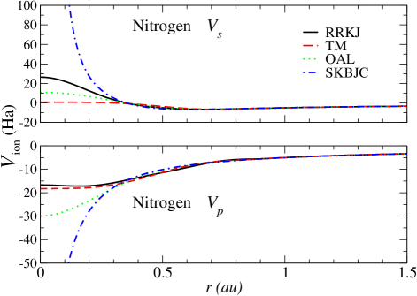
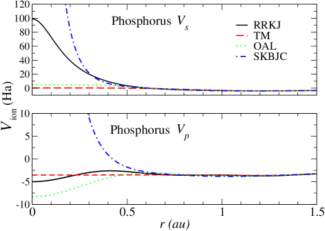
Figure 5: (Color online) Comparison of several ionic pseudopotentials for nitrogen and phosphorus. We show pseudopotentials obtained using the RRKJ, TM, OAL lester_psp , and the SBKJC EMSL methods. For the RRKJ and TM methods, the $r_{c}$ values are the same as those in Table 5. We show only the $s$ and $p$ potentials.

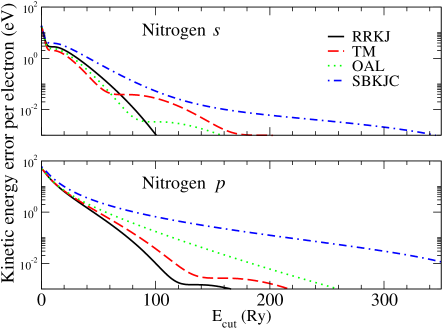
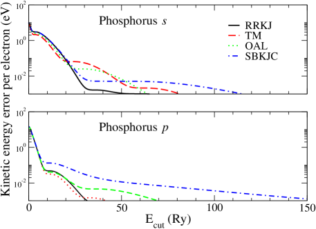
Figure 6: (Color online) Same as Fig. 5, except that we show the residual kinetic energy convergence (logarithmic scale) for the potentials calculated using Eq. (7).

Table 6: Planewave basis cutoff (in Ry) for nitrogen and phosphorus pseudopotentials for several pseudopotentials methods. The planewave basis cutoff is estimated using Eq. (7) for a residual kinetic energy of $\Delta T_{nl}\approx 5$ meV/electron, which can also be read from Fig. 6.

	Ecut(Ry)
	N	P
RRKJ	112	30
TM	145	50
OAL	210	55
SBKJC	375	90

Table 7: Dissociation energy $D_{e}$ in eV, bond length $R_{e}$ in Bohr, and harmonic frequency $\omega_{e}$ in cm^-1 for several dimers as calculated using density functional LDA and HF theories. We compare both the all-electron and the pseudopotential results. For each method, we generated the RRKJ pseudopotentials using the same level theory i.e. LDA and HF, respectively.

		LDA			HF
		AE	PSP		AE	PSP
N2	$D_{e}$	11.61	10.96		5.10	4.92
	$R_{e}$	2.07	2.06		2.01	2.02
	$\omega_{e}$	2388	2380		2720	2722
P2	$D_{e}$	6.25	6.02		1.70	1.70
	$R_{e}$	3.57	3.57		3.50	3.50
	$\omega_{e}$	794	788		912	905
Cl2	$D_{e}$	3.62	3.55		0.84	0.84
	$R_{e}$	3.74	3.74		3.73	3.72
	$\omega_{e}$	561	559		610	613

IV Study of several dimers

In this section, we apply our HF pseudopotentials in a study of three dimers and compare them with all-electron calculations. The pseudopotential calculations are done using a HF planewave basis code cpmd , and the all-electron results are obtained using a Gaussian basis code gaussian . For comparison, we have also generated LDA lda pseudopotentials using exactly the same parameters as those of the HF pseudopotential, and we compare them with their all-electron counterparts on an equal footing with the HF results. In our all-electron and pseudopotential results we used the Perdew-Wang lda flavor of LDA. We did not include a non-linear core correction (NLCC)nl_core ; nl_core_porezag in our LDA pseudopotentials for LDA/HF comparison purposes. The pseudopotential DFT calculations are carried out using ABINIT Abinit . The all-electron calculations are performed using the correlation-consistent cc-pV5Z basis set for N and cc-pV(5+d)Z for P and Cl dunning . The differences between the quadrupole and quintuple basis sets are negligible; e.g., in the binding energies the differences are less than 0.02 eV. We also verified these values using 6-311++G(3df,3pd) basis sets.

In Table 5, we show the cutoff radii we used to generate the RRKJ pseudopotentials for this study. These values, which are different from those of Table 1, are chosen to accommodate the bond lengths of these dimers without core overlap when possible. In the case of P and Cl, the $d$ core cutoff radius is allowed to extend beyond half of the dimer bond length to make softer pseudopotentials. The atomic reference configurations are the same as before.

Before presenting the molecular results, we comment on the planewave convergence of the RRKJ pseudopotentials in comparison to other pseudopotentials or ECPs. We examined the pseudopotentials of nitrogen and phosphorus as representatives of the first- and second-row elements. Figure 5 shows the RRKJ, TM, OAL lester_psp , and SBKJC EMSL pseudopotentials in real space for the two elements. We did not include a $d$-channel in these plots because neither the SBKJC nitrogen pseudopotential nor the OAL potentials have a $d$-channel. For the RRKJ and TM pseudopotentials, we used the cutoff radii as shown in Table 5. Note that the SBKJC ECP has a divergence at the origin, and is thus not suitable for planewave calculations. More generally, direct examination of pseudopotentials in real space gives little information about the planewave basis needed for converged eigenstates and eigenvalues.

One way to monitor the size of the planewave basis needed is to look at the residual kinetic energy convergence RRKJ of the pseudowavefunctions, which we show in Fig. 6. The residual kinetic energy is calculated as shown in Eq. (7) by varying $q_{c}$ (we plot it against $q_{c}^{2}$ which is the cutoff energy, for convenience). The planewave basis cutoff for each pseudopotential is determined by the potential channel requiring the largest cutoff energy. The estimated planewave basis cutoffs based on Fig. 6 are summarized in Table 6. As can be seen, RRKJ pseudopotentials give the smallest planewave basis cutoffs.

We summarize the results for the spectroscopic properties of the dimers in Table 7. The LDA and HF results for the equilibrium bond length and the harmonic vibrational frequencies of the dimers are shown to be well reproduced by both types of pseudopotentials. In the LDA dissociation energies there is a large discrepancy between all-electron and pseudopotential results for N₂, and to a lesser extent in P₂ and even much less in Cl₂. The HF pseudopotential dissociation energy of N₂ shows a significant deviation from the all-electron HF result, whereas for P₂ and Cl₂, the results are the same to within $0.01$ eV. A similar difference between all-electron and pseudopotential results was also seen in Ref. engel_exact_xc using the OPM method.

Most of errors in the LDA results are due to linear descreening of the pseudopotential, which is typically repaired by including a NLCC in the target calculation. Furthermore, because all three dimers are closed shell, the linear descreening effects are largest in the isolated atom calculations and therefore mostly affect the dissociation energies. As shown by Porezag et al. nl_core_porezag , these errors are larger for first row species compared to heavier atoms and increase with more unpaired electrons, explaining why N₂ has the largest error (first row, and 3 unpaired spins) and why Cl₂ (second row, 1 unpaired spin) has the smallest. Our LDA all-electron and pseudopotential energies are in excellent agreement with previous results engel_exact_xc without a NLCC. This study also showed that the all-electron results are in good agreement with the pseudopotentials values after including a NLCC, indicating that this is the dominant error for LDA pseudopotentials.

At the HF level there is also an error in the exchange contribution to the pseudopotential since the terms arising from core-valence interactions in the atomic reference state are frozen into the core and only valence-valence exchange terms are subtracted during the descreening step. As shown by our results and others shirley ; hock-engel , this type of descreening error is much smaller in magnitude in HF pseudopotentials compared to LDA. This would suggest that HF derived pseudopotentials are advantageous over those from LDA, at least in better descreening of the core-valence contributions.

V Summary and conclusion

Constructing HF pseudopotentials suitable for planewave calculations is a non-trivial task considering the extreme nonlocality of the exchange potential. Pseudopotentials constructed using a typical norm-conserving procedure develop a non-local and a non-Coulombic tail for large $r$. This would generally lead to erroneous results, especially in solid calculations. Several schemes have been introduced to cure the long tail behavior which lead to a small violation of the conservation of the core charge bk_exact_xc ; engel_exact_xc ; trail_needs1 .

In this study, we present soft-core HF pseudopotentials constructed using the RRKJ procedure which optimizes the potentials to yield rapid planewave basis cutoff convergence. The long tail behavior is fixed using a self-consistent procedure following that of Trail and Needs trail_needs1 , which leads to a negligibly small violation of norm-conservation. These pseudopotentials are applied in HF calculations of several atomic properties yielding results in good agreement with the all-electron values. We also apply them in the study of the dissociation energies, equilibrium bond lengths, and frequency of vibrations of several dimers, using a HF planewave code cpmd . The all-electron and pseudopotential results are in agreement with each other, and the values are consistent with a similar comparison done using LDA pseudopotential and LDA all-electron calculations.

Generation of HF based pseudopotentials has been released in version 3.0 of the GPL package OPIUM opium and is available for download.

VI Acknowledgments:

This work is supported by ONR grants N000140110365 and N000140510055, by the Department of Energy Office of Basic Energy Sciences grants DE-FG02-07ER15920 and DE-FG02-07ER46365, by the Air Force Office of Scientific Research, Air Force Materiel Command, USAF, Grant FA9550-07-1-0397 and by the NSF grant EAR-0530813. We are grateful to H. Krakauer and S. Zhang for many valuable discussions.

References

- (1) W. Kohn, Rev. Mod. Phys. 71, 1253 (1999).
- (2) For an excellent review see W. E. Pickett, Comput. Phys. Rep. 9, 115 (1989).
- (3) G. B. Bachelet, D. R. Hamann, and M. Schlüter, Phys. Rev. B 26, 4199 (1982).
- (4) A. M. Rappe, K. M. Rabe, E. Kaxiras, and J. D. Joannopoulos, Phys. Rev. B 41, R1227 (1990).
- (5) N. Troullier and J. L. Martins, Phys. Rev. B 43, 1993 (1991).
- (6) For a review of ECPs, see for example, M. Dolg, in Modern Methods and Algorithms of Quantum Chemistry, Proceedings, Second Edition, ed. J. Grotendorst, John von Newmann Institute for computing, Jülich, NIC Series, Vol 3 (2000).
- (7) J. S. Binkley, J. A. Pople, W. J. Hehre, J. Am. Chem. Soc. 102, 939 (1980); W. J. Stevens, H. Basch, M. Krauss, J. Chem. Phys. 81, 6026 (1984); W. J. Stevens, M. Krauss, H. Basch, P. G. Jasien, Can. J. Chem. 70, 612 (1992); T. T. Cundari and W. J. Stevens, J. Chem. Phys. 98, 5555 (1993).
- (8) P. J. Hay and W. R. Wadt, J. Chem. Phys. 82, 284 (1985); 82, 270 (1985); 82, 299 (1985).
- (9) P. A. Christiansen, Y. S. Lee, and K. S. Pitzer, J. Chem. Phys. 71, 4445 (1979).
- (10) M. Dolg, U. Wedig, H. Stoll, and H. Preuss, J. Chem. Phys. 86, 1866 (1987); J. Sheu, S. Lee, and M. Dolg, J. Chin. Chem. Soc. (Taipei) 50, 583 (2003).
- (11) C. W. Greeff and W. A. Lester, Jr., J. Chem. Phys. 109, 1607 (1998).
- (12) I. Ovcharenko, A. Aspuru-Guzik, and W. A. Lester, Jr., J. Chem. Phys. 114, 7790 (2001).
- (13) J. R. Trail and R. J. Needs, J. Chem. Phys. 122, 014112 (2005).
- (14) J. R. Trail and R. J. Needs, J. Chem. Phys. 122, 174109 (2005).
- (15) A. D. Becke, J. Chem. Phys. 98, 5648 (1993).
- (16) D. M. Bylander and L. Kleinman, Phys. Rev. Lett. 74, 3660 (1995); Phys. Rev. B 52, 14566 (1995); 54, 7891 (1996); 55, 9432 (1997).
- (17) M. Städele, J. A. Majewski, P. Vogl, and A. Görling, Phys. Rev. Lett. 79, 2089 (1997).
- (18) E. Engel, A. Höck, R. N. Schmid, R. M. Dreizler, and N. Chetty, Phys. Rev. B 64, 125111 (2001).
-
(19)
http://www.tcm.phy.cam.ac.uk/
~mdt26/casino2_pseudopotentials.html
- (20) C. F. Fischer, Comp. Phys. Comm. 98, 255 (1996).
- (21) G. S. Handler, D. W. Smith, and H. J. Silverstone, J. Chem. Phys. 73, 3936 (1980).
- (22) As in Ref. trail_needs1, , the deviation in the logarithmic derivative is computed neglecting changes in the Hartree and exchange potentials.
- (23) The logarithmic derivative is the ratio between the wavefunction and its slope, thus comparisons between logarithmic derivatives can be misleading if either value is close to zero. In all cases shown in Fig. 4, the magnitude of the wavefunctions and slopes ranged between and , respectively.
- (24) X. Gonze, R. Stumpf, and M. Scheffler, Phys. Rev. B 44, 8503 (1991).
- (25) OPIUM pseudopotential package http://opium.sourceforge.net.
- (26) E. Clementi and A. D. Mclean, Phys. Rev. 133, A419 (1963).; E. Clementi, A. D. Mclean, D. L. Raimondi, and M. Yoshimine, Phys. Rev. 133, A1274 (1963).
- (27) The ECPs are obtained from the Extensible Computational Chemistry Environment Basis Set Database (http://www.emsl.pnl.gov/forms/basisform.html).
- (28) CPMD version 3.9.2, Copyright IBM Corp 1990-2005, Copyright MPI für Festkörperforschung Stuttgart 1995-2001, http://www.cpmd.org.
- (29) Gaussian 98, Revision A.11.4, M. J. Frisch, G. W. Trucks, H. B. Schlegel, G. E. Scuseria, M. A. Robb, J. R. Cheeseman, V. G. Zakrzewski, J. A. Montgomery, Jr., R. E. Stratmann, J. C. Burant, S. Dapprich, J. M. Millam, A. D. Daniels, K. N. Kudin, M. C. Strain, O. Farkas, J. Tomasi, V. Barone, M. Cossi, R. Cammi, B. Mennucci, C. Pomelli, C. Adamo, S. Clifford, J. Ochterski, G. A. Petersson, P. Y. Ayala, Q. Cui, K. Morokuma, N. Rega, P. Salvador, J. J. Dannenberg, D. K. Malick, A. D. Rabuck, K. Raghavachari, J. B. Foresman, J. Cioslowski, J. V. Ortiz, A. G. Baboul, B. B. Stefanov, G. Liu, A. Liashenko, P. Piskorz, I. Komaromi, R. Gomperts, R. L. Martin, D. J. Fox, T. Keith, M. A. Al-Laham, C. Y. Peng, A. Nanayakkara, M. Challacombe, P. M. W. Gill, B. Johnson, W. Chen, M. W. Wong, J. L. Andres, C. Gonzalez, M. Head-Gordon, E. S. Replogle, and J. A. Pople, Gaussian, Inc., Pittsburgh PA, 2002.
- (30) J. P. Perdew and Y. Wang, Phys. Rev. B 45, 13244 (1992).
- (31) X. Gonze, J. -M. Beuken, R. Cara-cas, F. Detraux, M. Fuchs, G. -M. Rignanese, L. Sindic, M. Verstraete, G. Zerah, F. Jollet, M. Torrent, A. Roy, M. Mikami, Ph. Ghosez, J. -Y. Raty, and D. C. Allan, Comp. Mat. Sci. 25, 478 (2002).
- (32) T. H. Dunning, J. Chem. Phys. 90, 1007 (1989); T. H. Dunning, Jr., K. A. Peterson, and A. K. Wilson, J. Chem. Phys. 114, 9244 (2001).
- (33) S. G. Louie, S. Froyen, and M. L. Cohen Phys. Rev. B 26, 1738 (1982).
- (34) D. Porezag, M. R. Pederson, and A. Y. Liu , Phys. Rev. B 60, 14132 (1999).
- (35) E. L. Shirley, R. M. Martin, G. B. Bachelet, and D. M. Ceperley, Phys. Rev. B 42, 5057 (1990).
- (36) A. Höck and E. Engel, Phys. Rev. A 58, 3578 (1998).