Dispersion Terms and Analysis of Size- and Charge- Dependence in an Enhanced Poisson-Boltzmann Approach

Abstract

We implement a well-established concept to consider dispersion effects within a Poisson-Boltzmann approach of continuum solvation of proteins. The theoretical framework is particularly suited for boundary element methods. Free parameters are determined by comparison to experimental data as well as high level Quantum Mechanical reference calculations. The method is general and can be easily extended in several directions. The model is tested on various chemical substances and found to yield good quality estimates of the solvation free energy without obvious indication of any introduced bias. Once optimized, the model is applied to a series of proteins and factors such as protein size or partial charge assignments are studied.

Department of Physics, Michigan Technological University, 1400 Townsend Drive, Houghton, MI, 49931-1295, USA, and John von Neumann Institute for Computing, Forschungszentrum Jülich, 52425 Jülich, Germany

RECEIVED DATE (to be automatically inserted)

Keywords: Poisson-Boltzmann, Dispersion, Boundary Element Method, Solvation Free Energy, Polarizable Continuum Model;

1 Introduction

The stabilizing effect of water on biomolecules is an intensively studied area in contemporary biophysical research. This is because many of the key principles governing biological functionality result from the action of the solvent, and thus water is often regarded as the “matrix of life”.

In theoretical work, the important factor “solvent” needs to be taken into account too, or the studied system will be unphysical. There are two main ways of solvent treatment in biophysical research. One is to embed the biomolecule of interest into a box of explicit solvent molecules resolved into full atomic detail ^{1, 2, 3}. The alternative form is to consider the solvent as structureless continuum and describe the response of the environment with implicit solvation methods ^{4, 5, 6, 7, 8}. Much effort has been devoted to describing the electrostatic component within implicit solvation models. Efficient solutions have become popular in the form of Generalized Born (GB) models ^{9, 10, 11, 12} as well as Poisson-Boltzmann models (PB) ^{13, 14, 15, 16, 17, 18, 19, 20}. Solutions to the PB are computed either by the finite difference method (FDPB) ^{13, 14, 15, 16} or by the boundary element method (PB/BEM) ^{19, 20}. Considerable computational savings are expected from the latter because the problem can be reduced from having to solve a volume integral in FDPB to solving a surface integral in PB/BEM. Either approach is sensitive to the degree of discretization into grid elements or boundary elements ^{21, 22}.

Aside from the electrostatic component there are also apolar contributions to consider ^{4, 23}. Especially in the context of nonpolar molecules, such factors often become the dominant terms in the solvation free energy. A common way to treat these nonpolar contributions is to introduce a SASA-term, which means measuring the solvent accessible surface area (SASA) and weighing it with an empirically determined factor. Although commonly employed, this procedure has become the subject of intensive debates ^{24, 25, 26, 27}. Not only were SASA terms found to be inappropriate for representing the cavitation term ^{34, 27}, but also is the weighing factor — usually associated with surface tension — completely ill-defined in an atomic scale context ³⁵. While the short range character of dispersion and repulsion forces occurring at the boundary between solute and solvent would imply that SASA can describe these kinds of interactions, a recent careful analysis has shown that at least for dispersion such a relationship is not justified ²⁴.

The discrepancy arising with SASA-terms has been recognized by many groups and its persistent employment may be largely due to sizeable cancellation of error effects. Wagoner and Baker ²⁷ have devided the non-polar contributions into repulsive and attractive components and compared their approach to mean forces obtained from simulation data on explicitly solvated systems. The specific role of the volume to account for repulsive interactions (cavitation) was clearly identified. Further inclusion of a dispersion term resulted in a satisfactory model of high predictive quality. Levy and Gallicchio devised a similar decomposition into a SASA-dependent cavitation term and a dispersion term within a GB scheme ^{28, 29, 30}. Their model makes use of atomic surface tensions and a rigorous definition of the molecular geometry within the GB framework. Particularly attractive is their efficient implementation and straightforward interfacing with Molecular Dynamics codes. Zacharias has already noted that a decompositon into a dispersion term and a SASA-based cavity term greatly benefits the quality of predictions of apolar solvation ²³. His approach uses distinct surface layers for either contribution. Hydration free energies of a series of tested alkanes agreed very well with data from explicit simulations ³¹ and from experiment. The striking feature in this approach is the improvement in hydration free energies of cyclic alkanes. Methodic advancement has recently been reported within the newest release of AMBER ³⁶ where GB was augmented by a volume term ³⁷ and the inclusion of dispersion terms was found to significantly improve the general predictive quality of PB. Of particular interest are systematic and physics-based decompositions that allow for separate consideration of each of the terms involved. In Quantum Mechanics (QM) such a technique has long been established with the Polarizable Continuum Model (PCM) ⁴. It therefore seems advisable to use techniques like PCM as a reference system whenever additional method development is performed, especially when regarding the multitude of technical dependencies continuum solvation models are faced with ^{21, 22}.

In the present work we describe a systematic process to introduce dispersion terms in the context of the PB/BEM approach. The PCM model, that treats dispersion and repulsion terms from first-principles, is used as a reference system along with experimental data. Different ways of calculating dispersion-, repulsion contributions in PCM have recently been compared ³⁸. For our purposes the Caillet-Claverie method ^{39, 40} was implemented since it seems to offer a good compromise between accuracy and computational overhead. This method was also chosen in earlier versions of PCM ⁴¹ and thus represents a proven concept within the BEM framework. The fundamental role of dispersion and the potential danger of misinterpreting hydrophobicity related phenomena by ignoring it has been underlined recently ^{42, 43}. Given the fundmental nature of hydrophobicity and the potential role of dispersion within it together with the current diversity seen in all the explanatory model concepts ^{44, 45} it seems to be necessary to advance all technical refinements to all solvation models (implicit as well as explicit) just to facilitate an eventual understanding of the factors governing these basic structure-forming principles.

After determination of appropriate dispersion constants used in the Caillet-Claverie approach we apply our model to a series of proteins of increasing size. In this way we can analyze the relative contribution of the individual terms as a function of system size. Moreover, we have carried out semi-empirical calculations on the same series of proteins and can therefore compare effects resulting from different charge assignments to each other. The semi-empirical program LocalSCF ⁴⁶ also allowed for estimation of the polarization free energies according to the COSMO model ⁴⁷, which could be readily used for direct comparison to PB/BEM data.

2 Methods

2.1 Theoretical Concepts

We use the following decomposition of the solvation free energy

$$\Delta G^{solv}=\Delta G^{pol}+\Delta G^{cav}+\Delta G^{disp}$$ (1)

where the individual terms represent polarization, cavitation and dispersion contributions. Explicit consideration of repulsion is not necessary as the cavitation term includes these interactions. PB/BEM methodology is used for $\Delta G^{pol}$ at the boundary specification described previously ²². The cavitation term is expressed via the revised Pierotti approximation ^{34, 35} (rPA), which is based on the Scaled Particle Theory ^{32, 33}. The major advantage with this revised approximation is a transformation property involving the solvent excluded volume. Hence after having identified the basic rPA-coefficients from free energy calculations the rPA-formula may be applied to any solute regardless of its particular shape or size ³⁴. $\Delta G^{disp}$ is computed from the Caillet-Claverie formula ^{39, 40} projected onto the boundary elements as suggested by Floris et al. ⁴¹

$$\Delta G^{disp}=\sum\limits_{i}^{I}\rho^{slv}\omega_{i}\sum\limits_{j}^{J}\sum\limits_{k}^{K}\underbrace{-0.214\kappa_{i}\kappa_{j}\frac{64(R_{i}^{W})^{3}(R_{j}^{W})^{3}}{{R_{ij}}^{6}}}_{Caillet-Claverie}\frac{1}{3}\left(\vec{R}_{ij}\cdot\vec{n}_{k}\right)\Delta\sigma_{k}$$ (2)

where the first sum is over different atom types, $i$, composing one molecule of solvent, the second sum is over all solute atoms, $j$, and the sum over $k$ is over all surface elements resulting from an expansion of the molecular surface by the dimension of radius $R_{i}^{W}$ of a particular solvent atom, see Figure 1 for a graphical representation. Here solvent atoms are shown in grey and solute atoms are represented as white circles. The scheme corresponds to one particular choice of $i$. For example, if the solvent molecule in Figure 1 is water, then the scenery depicts the first of two possibilities where $i$ refers to the oxygen atom. After $i$ is set, all atom radii of the solute are increased by the amount of the atomic radius of oxygen and the molecular surface (dashed line in Figure 1) is reconstructed. Next the inner double sum is carried out where $J$ is the total number of solute atoms and $K$ is the total number of BEs forming the interface. Note that index $j$ serves for a double purpose, looping over all solute atoms as well as defining the type of atomic radius to use. At every combination $j,k$ of solute atoms with BEs, the expression emphasized by the curly bracket in eq. 2 must be evaluated. Here $\kappa_{i}$ and $\kappa_{j}$ are dispersion coefficients and $R_{i}^{W}$, $R_{j}^{W}$ are atomic radii, all of them determined empirically by Caillet-Claverie ^{39, 40}. The corresponding values are summarized in Table 1. $R_{ij}$ is the distance between the center of some BE, $k$, and the center of a solute atom, $j$. After the expression in the curly bracket of eq. 2 has been evaluated it must be multiplied with a scalar product between the vectors $\vec{R}_{ij}$ and $\vec{n}_{k}$, the inwards pointing normal vector corresponding to the $k^{th}$ BE. The remainder of eq. 2 is multiplication with a constant factor $\frac{1}{3}$ and multiplication with $\Delta\sigma_{k}$, the partial area of the BE, $k$. After all possible combinations $j,k$ have been considered, the procedure is repeated with an incremented $i$, now referring to the H-atom, the second type of atom in a molecule of water. The molecular surface is recomputed, extended by the dimension of the atomic radius of hydrogen, and the entire inner double sum will be repeated as outlined for the case of oxygen. However, since both H-atoms in the solvent molecule are identical this step needs to be done only once and $\omega_{i}$, the number of occurrences of a particular atom type $i$, will take care of the rest (in the case of water $\omega_{1}=1$ for oxygen and $\omega_{2}=2$ for hydrogen). Finally, $\rho^{slv}$ in eq. 2 represents the number density of the solvent. We have restricted the approach to just the 6^th-order term in the expression derived by Floris et al. ⁴¹. Note that we consider molecular surfaces as defined by Connolly ⁴⁸. The partial term listed after the curly bracket in eq. 2 is the actual consequence of mapping the classical pair interaction terms onto a boundary surface ⁴¹. The partial expression enclosed in the curly bracket can be substituted with any other classic pair potential, for example using AMBER style of dispersion ³⁶,

$$\Delta G^{disp}=\sum\limits_{i}^{I}\rho^{slv}\omega_{i}\sum\limits_{j}^{J}\sum\limits_{k}^{K}\underbrace{-2\sqrt{\epsilon_{i}\epsilon_{j}}\left(\frac{R_{i}^{W}+R_{j}^{W}}{R_{ij}}\right)^{6}}_{AMBER}\frac{1}{3}\left(\vec{R}_{ij}\cdot\vec{n}_{k}\right)\Delta\sigma_{k}$$ (3)

with similar meanings of the variables used above and $\epsilon_{i}$ being the van der Waals well depth corresponding to homogeneous pair interaction of atoms of type $i$.

2.2 Model Calibration

The algorithm covering computation of dispersion is implemented in the PB/BEM program POLCH ⁴⁹ (serial version). Proper functionality was tested by comparing dispersion results of 4 sample molecules, methane, propane, iso-butane and methyl-indole, against results obtained from GAUSSIAN-98 ⁵⁰ (PCM model of water at user defined geometries). Deviations were on the order of $\pm$ 1.8 % of the G98 value, so the procedure is assumed to work correctly. The small variations are the result of employing a different molecular surface program in PB/BEM ⁵¹. Next the structures of amino acid side-chain analogues are derived from standard AMBER pdb ⁵⁶ geometries by making the C_α-atom a hydrogen atom, adjusting the C-H bond length and deleting the rest of the pdb structure except the actual side chain of interest. In a similar process, zwitterionic forms of each type of amino acid are constructed. PB/BEM calculations are carried out and net solvation free energies for solvent water are stored. A comparison is made against the experimental values listed in ⁵² as well as results obtained from the PCM model in GAUSSIAN-03 ⁵³. AMBER default charges and AMBER van der Waals radii increased by a multiplicative factor of 1.07 are used throughout ²². Initial deviation from the reference set is successively improved by introducing a uniform scaling factor to the dispersion coefficients $\kappa_{i}$ of eq. 2. The optimal choice of this dispersion scaling factor is identified from the minimum mean deviation against the reference data set. The initially derived optimal scaling factor is applied to the zwitterionic series, a subset of molecules for which experimental values have been compiled ⁵⁴, and a set of 180 dipeptide conformations studied previously. When new molecules are parameterized, we use ANTECHAMBER from AMBER-8 and RESP charges based on MP2/6-31g* grids of electrostatic potentials ⁵⁵. Molecular geometries are optimized in a two-step procedure, at first at B3LYP/3-21g* and then at MP2/6-31g* level of theory and only the final optimized structure becomes subject to the RESP calculation.

Extensions are pursued in two directions. First, the PB/BEM approach is used with solvents other than water, and the question is raised whether the optimized scaling factor for dispersion in water is of a universal nature or needs to be re-adjusted for each other type of solvent considered. Secondly, we tested the introduced change when the Caillet-Claverie specific formalism of dispersion treatment is changed to AMBER-style dispersion as indicated in eqs. 2 and 3.

2.3 Study of Size- and Charge Dependence

Crystal structures of 10 proteins of increasing size are obtained from the Protein Data Bank ⁵⁶. The actual download site is the repository PDB-REPRDB ⁵⁷. Structures are purified and processed as described previously ⁵⁸. The PDB codes together with a characterization of main structural features of the selected test proteins are summarized in Table 2. Two types of calculations are carried out using the semi-empirical model PM5 ⁵⁹ and the fast multipole moment (FMM) method ⁶⁰. A single point vacuum energy calculation is followed by a single point energy calculation including the COSMO model ⁴⁷ for consideration of solvent water. The difference between the two types of single point energies should provide us with an estimate of the solvation free energy. Furthermore, the finally computed set of atomic partial charges is extracted from the PM5-calculation and feeded into the PB/BEM model to substitute standard AMBER partial charges. In this way we can examine the dependence on a chosen charge model as well as compare classic with semi-empirical QM approaches to the solvation free energy.

2.4 Computational Aspects

The sample set of 10 proteins listed in Table 2 is analyzed with respect to computational performance regarding the calculation of the dispersion term as defined in eq. 3. It is important to note that for this particular task the surface resolution into BEs may be lowered to levels where the average size of the BEs becomes $\approx$ 0.45 Ų. CPU times for the two steps, ie creation and processing of the surface and evaluation of the expression for $\Delta G^{disp}$ are recorded and summarized in Table XII of the Supplementary Material. As can be seen clearly from these data, the major rate-limiting step is the production of the surface, which can reach levels of up to 20 % of the total computation time. Evaluation of the dispersion term itself is of negligible computational cost. Since the surface used for the polarization term is defined according to Connolly (see section 2.1), we could not use this molecular surface directly for a SASA-based alternative treatment of the non-polar contributions. Rather we had to compute a SASA from scratch too, and were facing identical computational constraints as seen with the approach chosen here.

3 Results

3.1 A universal scaling factor applied to Caillet-Claverie dispersion coefficients leads to good overall agreement with experimental solvation free energies of amino acid side-chain analogues in water

Since our main focus is on proteins, our first goal is to optimize our approach for proteins in aqueous solution. We can resort to the experimental data for amino acid side-chain analogues (see ⁵² and references therein). At first we seek maximum degree of agreement between experimental and PB/BEM values of the solvation free energy, $\Delta G^{solv}$, by multiplying a scaling factor, $\lambda$, to the Caillet-Claverie dispersion ^{39, 40} coefficients, $\kappa_{i}$. The remaining terms in eq. 1 are computed at the optimized conditions reported previously ^{22, 35}. We define a global deviation from the experimental data by

$$\Delta\Delta G^{solv}=\frac{1}{13}\sum\limits_{i=1}^{13}\sqrt{\left(\Delta G^{solv,Exp}_{i}-\Delta G^{solv,PB/BEM}_{i,\lambda}\right)^{2}}$$ (4)

where $i$ refers to a particular type of amino acid side-chain analogue included in the reference set of experimental values and $\lambda$ is the introduced scaling factor applied to the Caillet-Claverie dispersion ^{39, 40} coefficients. The trend of $\Delta\Delta G^{solv}$ for different choices of $\lambda$ is shown in Figure 2. As becomes clear from Figure 2, a scaling factor of 0.70 establishes the best match to the experimental data. A detailed comparison of individual amino acid side-chain analogues at this optimum value is given in Table 3. We achieve a mean unsigned error of 1.15 $\frac{kcal}{mol}$, hence come close to the accuracy reported recently by Chang et al. ⁵², a study that agreed very well with earlier calculations carried out by Shirts et al. ⁶¹ and MacCallum et al. ⁶². Several computed solvation free energies in Table 3 still show significant deviation from the experimental value, e.g. p-cresol and methanethiol. A comparison to results with a simple SASA-based model is included in the Supplementary Material (Table XI). This comparison reveals a certain improvement for the most critical components, but no indication of a general amelioration of the situation. The somewhat special character of methanethiol has been noticed before ²⁵.

3.2 Component-wise juxtaposition of PB/BEM and PCM approaches reveals a difference in individual contributions but similarity in net effects

As interesting as total solvation free energies are the constituting partial terms and how they compare to their analogous counter parts in a high-level QM model such as PCM. We therefore studied all amino acid side-chain analogues with PCM ⁴ calculations at the Becke-98 ⁶³ level of density functional theory (DFT) using the high-quality basis set of Sadlej ⁶⁴ and program GAUSSIAN-03 ⁵³. A summary of these data is given in Table 4. Since in PB/BEM we do not consider repulsion explicitly, the PB/BEM dispersion term is compared to the sum of $\Delta G^{disp}$ and $\Delta G^{rep}$ of PCM. It becomes clear from Table 4 that there is rather general agreement in polarization terms but sizeable divergence in the apolar terms. However, the sum of all apolar terms, ie. $\Delta G^{cav}$ and $\Delta G^{disp}$, appears to be again in good agreement when comparing PB/BEM with PCM. The reason for the difference in the apolar terms is largely due to a different cavitation formalism used in PB/BEM, which we currently believe to represent a very good approximation to this term ³⁵.

3.3 The identified scaling factor of 0.70 applied to Caillet-Claverie dispersion coefficients yields good quality estimates of the solvation free energy in water for many molecules

In order to test the PB/BEM approach further we used the initially determined scaling factor for dispersion coefficients of 0.70 to compute water solvation free energies of a series of other molecules. The procedure for obtaining atomic partial charges is described in section 2.2. It is important to note that the electron density used for RESP fitting must be of MP2/6-31G* quality to achieve maximum degree of compatibility to standard AMBER charges, which have been found to mimic high quality calculations very well ²². Experimental reference values have been obtained from the extensive compilation by Li et al. ⁵⁴. The data comprising 18 arbitrarily selected molecules are summarized in Table 5. The mean unsigned error of 1.18 $\frac{kcal}{mol}$ for this set of molecules comes close to PCM quality and must be considered very satisfactory again.

Another class of molecules we looked into are amino acids in their zwitterionic form, where due to the charges at the amino/carboxy groups the net solvation free energies become larger by about an order of magnitude. A comparison against the recently reported data by Chang et al. ⁵² is given in Table 6. The degree of agreement is still considerably high and there is no obvious indication of a systematic deviation.

A final comparison is made against a series of 180 molecules that has been used in a previous study ²². These structures include all 20 types of naturally occurring amino acids in 9 different conformations (zwitterionic forms assumed). The set of dipeptides has been subjected to PCM ⁴ calculations at the Becke-98 DFT level ⁶³ using Sadlej’s basis set ⁶⁴. Average net solvation free energies are formed from all 9 different conformations per type of amino acid (or the number of available reference calculations) and the results are presented in Table I in the supplementary material. Considering the variation with respect to conformational flexibility the match must still be considered to be reasonably good. It is interesting to note that the variability of the dispersion contributions alone, considered isolated per se as a function of conformational flexibility is much less pronounced than what we see for the net solvation (see Table II of the supplementary material).

3.4 The scaling factor of 0.70 applied to Caillet-Claverie dispersion coefficients in the case of water is not of a universal nature but must be re-optimized for any other type of solvent.

An important aspect of the PB/BEM approach is how the identified scaling factor for Caillet-Claverie dispersion coefficients — 0.70 in the case of water — translates into other situations of non-aqueous solvation. We have therefore repeated the studies for identifying optimal boundaries ²² for solvents methanol, ethanol and n-octanol. Again we consider PCM cavities of the set of 180 dipeptide structures as reference systems and search for the best match in volumes and surfaces dependent on slightly enlarged or shrinked standard AMBER van der Waals radii. We again employ the molecular surface program SIMS ⁵¹. Detailed material of this fit is included in the supplementary material (Tables III-VIII and Figures I-VI). We find to have to marginally increase AMBER van der Waals radii by factors of 1.06 in solvents methanol and ethanol and 1.05 in solvent n-octanol. Based on these conditions for proper locations of the solute-solvent interface we then repeat the search for appropriate scaling factors of dispersion coefficients that result in close agreement to experimental solvation free energies (see section 3.1). Results are presented in Figures 3 and 4. It becomes clear that the factor of 0.70, optimal for water, is not universally applicable. Rather, we find for ethanol 0.82 and for n-octanol 0.74 to be the optimal choices. A detailed comparison against experimental values at optimized conditions is given in Tables 7 and 8. We achieve mean unsigned errors of 1.38 $\frac{kcal}{mol}$ for ethanol and 1.27 $\frac{kcal}{mol}$ for n-octanol. Cavitation terms of similar quality to the ones presented in ³⁵, which are needed in PB/BEM, are available for methanol and ethanol (unpublished work in progress) or obtained from ⁶⁵. Unfortunately, we cannot do the calculations for methanol because of the lack of experimental values and the non-systematic trend in dispersion scaling factors of the other alcoholic solvents. All optimized parameter sets for the various types of solvents are summarized in Table 9.

3.5 Switching from Caillet-Claverie-style of dispersion to AMBER-style requires a re-adjustment of scaling factors.

An obvious question is how the described approach will change when substituting the Caillet-Claverie formalism with the corresponding AMBER-dispersion formula, ie replacing eq. 2 with eq. 3. We therefore implemented a variant where we use eq. 3 together with standard AMBER van der Waals radii (slightly increased as done for the definition of the boundary and indicated in table 9) and standard AMBER van der Waals potential well depths. Similar to the Caillet-Claverie treatment we find that a uniform scaling factor, $\lambda$, applied to the AMBER van der Waals potential well depths, $\epsilon_{i}$, is sufficient to lead to good agreement with experimental data. An identical strategy to the one presented in section 3.1 for determination of appropriate values of $\lambda$ may be applied. The optimal choice of $\lambda$ turns out to be 0.76 for solvent water as indicated in Figure IX of the Supplementary Material. Corresponding detailed data is shown in Table 10. The mean unsigned error amounts to 1.01 $\frac{kcal}{mol}$ at optimized conditions. While in the case of water similar scaling factors are obtained for Caillet-Claverie as well as AMBER type of dispersion, for the remaining types of solvents a less coherent picture arises (see Table 9). Identification of scaling factors for solvents ethanol ($\lambda$=0.94) and n-octanol ($\lambda$=2.60) is shown in Figures X and XI of the Supplementary Material and corresponding detailed data listed in Tables IX and X of the Supplementary Material. Mean unsigned errors are 1.21 $\frac{kcal}{mol}$ for ethanol and 1.00 $\frac{kcal}{mol}$ for n-octanol respectively. Either approach is competitive and comes with its own merits. Caillet-Claverie coefficients are more general and specific to chemical elements only, hence no distinction between for example sp3-C atoms and sp2-C atoms needs to be made. Employment of AMBER parameters on the other hand appears to be straightforward in the present context since the geometry of the boundary is already based on AMBER van der Waals radii.

3.6 Replacement of static AMBER partial charges with semi-empirical PM5 charges introduces a rise in solvation free energies by about 20 % of the classic result regardless of the size or total charge state of the system.

A series of proteins of different size, shape and total net charge (see Table 2) is computed within the PB/BEM approach at optimized conditions for aqueous solvation, that is using a Caillet-Claverie dispersion coefficient scaling factor of 0.70, slightly increased AMBER van der Waals radii by a factor of 1.07 and standard AMBER partial charges. In addition to this classic approximation we also carry out semi-empirical QM calculations with the help of program LocalSCF ⁴⁶ using the PM5 model. From the semi-empirical calculation we extract atomic partial charges and use these instead of AMBER partial charges within the PB/BEM approach. Results of these calculations are presented in Table 11 and Figure 5. In general one can observe a rather constant change of about 20 % of the classic AMBER based $\Delta G^{solv}$ estimate when switching to PM5 charges. This is independent of the size, shape or net charge of the system (compare red bars with purple bars in Figure 5). The polarization term constitutes the major contribution but apolar terms are far from negligible (compare magnitude of blue and black bars to green and grey bars in Figure 5). When using the COSMO approximation within the semi-empirical method and deriving solvation free energies from that we get entirely uncorrelated results for the solvation free energy, $\Delta G^{solv}$ (see 9^th column in Table 11). It is important to note that the surface to volume ratio drops to a value around 0.25 with increasing protein size, whereas typical values in the range of 0.80 to 1.0 are maintained in the initial calibration phase, hence care must be taken with large scale extrapolations from small molecular reference data.

4 Discussion

Motivated by our recent high-performance implementation of Poisson-Boltzmann calculations ⁴⁹ we now complement this approach with a systematic inclusion of apolar effects. In particular the important dispersion contribution is introduced and fine-tuned against available experimental data. This is based on physics-based terms, that have long been considered in a similar fashion within QM models ⁴. The resulting model is applied to a series of protein structures, and size and charge effects are examined.

Direct assessment of the predictive quality of the PB/BEM approach after calibration has revealed rather good performance indicators for PB/BEM. This was based on suggested scaling factors applied to Caillet-Claverie dispersion coefficients. Since the original aim of Caillet-Claverie was to explain crystal data, we would expect a need for re-adjustment in this present implementation. Moreover, since the boundary and the rest of the PB/BEM model is based on AMBER parameterization it does not come as a surprise that one has to adjust a non-related second set of van der Waals parameters in order to achieve general agreement to a reference data set. Related to this point it seems particularly encouraging that when replacing the scaled Caillet-Claverie part with standard AMBER-dispersion terms for water no further refinement is necessary and similar levels of precision are established automatically. In the case of water, this brings in a second advantage. Because the employed TIP3P model assigns van der Waals radii of zero to the H-atoms, so the effective sum over $i$ in eq. 3 may be truncated already after the oxygen atom. The second cycle considering H-atoms in water would add only zeros any more.

A somewhat critical issue is the determination of missing parameters or the estimation of solvent probe sphere radii for different types of solvents. In this present work we found it convenient to make use of electron density grids and corresponding iso-density thresholds to define the boundary of molecules. For example to determine the probe sphere radius of methanol we compute the volume of a single molecule of methanol up to an electron density threshold of 0.0055 a.u. and derive an effective radius assuming spherical relationships. The same threshold criterion is applied to all other solvents leading to the data summarized in Table 9. Electron grids are based on B98/Sadlej calculations. Similarly we determine atomic van der Waals radii for Cl- or Br-containing substances from iso-density considerations. However in these latter cases the threshold criterion is adapted to a level that re-produces proper dimensions of well-known types, ie neighboring C-, O-, N-atoms and at this level the unknown radius is determined. In the case of n-octanol the assumption of spherical geometry is certainly not justified. On the other hand the concept of an over-rolling probe sphere representing approaching solvent molecules will remain a hypothetical model construct anyway. Complying with this model construct it may be argued that over time the average of approaching solvent molecules will hit the solute with all parts (head, tail or body regions of the solvent molecule) equally often and thus the idealized spherical probe is not entirely unreasonable.

Another interesting aspect is the fact that the present PB/BEM approach is all based on molecular surfaces rather than SASAs. This is of technical interest and the consequence of that is a greatly reduced sensitivity to actual probe sphere dimensions. A graphical explanation is given in the supplementary material (Figure VII). While SASA based surfaces would see significant changes when probe spheres are slightly modified (blue sphere replaced by red sphere in Figure VII of the supplementary material) the molecular surface itself faces only a minor change in the reentrant domain (green layer indicated in Figure VII of the supplementary material).

Large scale extrapolations resulting from a calibration process done with small sized reference structures have to be taken with care. Because of the drop of surface to volume ratios the most important requirement for such a strategy is to have the individual terms properly analyzed whether they scale with the volume, or the surface. For PB/BEM the question reduces to the cavitation term, since the remainder is mainly a function of Coulombic interactions. As that particular aspect has been carefully analyzed in previous studies ³⁴ we are confident that a large-scale extrapolation actually works in the way suggested in eq. 1.

A final remark may be relevant with regard to the discrepancy seen in using classic AMBER partial charges versus semi-empirical PM5 charges. Intuitively, one is tempted to believe stronger in the PM5 results. There might however also be a small drift in energies introduced by PM5/PM3 models as has been observed within an independent series of single point calculations (see supplementary material Figure VIII).

5 Conclusion

Consideration of dispersion effects within a physics-based continuum solvation model significantly improves accuracy and general applicability of such an approach. The proposed method follows a proven concept ⁴¹ and is easily implemented into existing models. Generalization to different treatments of dispersion as well as extension to non-aqueous solvents is straightforward.

6 Acknowledgements

This work was supported by the National Institutes of Health Grant GM62838. We thank FQS Poland and the FUJITSU Group, for kindly providing a temporary test version of program LocalSCF ⁴⁶.

Table 1: Summary of the data used for Caillet-Claverie style of dispersion treatment as outlined in eq. 2.

Caillet-Claverie Dispersion Coefficients, $\kappa$, and Atomic Radii, $R^{W}$, in Å39, 40
$\kappa_{H}$	$\kappa_{C}$	$\kappa_{N}$	$\kappa_{O}$	$\kappa_{F}$	$\kappa_{Na}$	$\kappa_{P}$	$\kappa_{S}$	$\kappa_{Cl}$	$\kappa_{K}$	$\kappa_{Br}$	$\kappa_{J}$
1.00	1.00	1.18	1.36	1.50	1.40	2.10	2.40	2.10	2.90	2.40	3.20
$R_{H}^{W}$	$R_{C}^{W}$	$R_{N}^{W}$	$R_{O}^{W}$	$R_{F}^{W}$	$R_{Na}^{W}$	$R_{P}^{W}$	$R_{S}^{W}$	$R_{Cl}^{W}$	$R_{K}^{W}$	$R_{Br}^{W}$	$R_{J}^{W}$
1.20	1.70	1.60	1.50	1.45	1.20	1.85	1.80	1.76	1.46	1.85	1.96

Table 2: PDB codes and structural key data of a series of proteins used for comparison

Shape Sketch	PDB-Code	Number of	Number of	Charge
		Residues	Atoms	[a.u.]
	1P9GA	41	517	+3
	2B97	70	981	+1
	1LNI	96	1443	-5
	1NKI	134	2082	+5
	1EB6	177	2570	-11
	1G66	207	2777	-2
	1P1X	250	3813	0
	1RTQ	291	4287	-16
	1YQS	345	5147	+2
	1GPI	430	6164	-12

Table 3: Comparison of PB/BEM-computed versus experimental total solvation free energies, $\Delta G^{solv}$, of amino acid side-chain analogues in water. A scaling factor, $\lambda$, of 0.70 has been uniformly applied to all dispersion coefficients, $\kappa_{i}$, in eq. 2.

Species	$\Delta G^{solv,PB/BEM}$	$\Delta G^{solv,Exp}$	Deviation
	$\left[\frac{kcal}{mol}\right]$	$\left[\frac{kcal}{mol}\right]$	$\left[\frac{kcal}{mol}\right]$
acetamide	-10.97	-9.68	1.29
butane	1.92	2.15	0.23
ethanol	-4.58	-4.88	0.30
isobutane	1.74	2.28	0.54
methane	0.72	1.94	1.22
methanethiol	-3.57	-1.24	2.33
methanol	-6.58	-5.06	1.52
methyl-ethyl-sulfide	-0.30	-1.48	1.18
methylindole	-4.19	-5.88	1.69
p-cresol	-3.56	-6.11	2.55
propane	1.72	1.99	0.27
propionamide	-9.34	-9.38	0.04
toluene	1.05	-0.76	1.81

Table 4: Analysis of individual contributions to the net solvation free energy for solvent water as computed by PB/BEM or by PCM and comparison to the experimental value.

Species	$\Delta G^{cav}$	$\Delta G^{cav}$	$\Delta G^{disp}$	$\Delta G^{disp}_{rep}$	$\Delta G^{pol}$	$\Delta G^{pol}$	$\Delta G^{solv}$	$\Delta G^{solv}$	$\Delta G^{solv}$
	PB/BEM	PCM	PB/BEM	PCM	PB/BEM	PCM	PB/BEM	PCM	Exp
	$\left[\frac{kcal}{mol}\right]$	$\left[\frac{kcal}{mol}\right]$	$\left[\frac{kcal}{mol}\right]$	$\left[\frac{kcal}{mol}\right]$	$\left[\frac{kcal}{mol}\right]$	$\left[\frac{kcal}{mol}\right]$	$\left[\frac{kcal}{mol}\right]$	$\left[\frac{kcal}{mol}\right]$	$\left[\frac{kcal}{mol}\right]$
acetamide	5.10	12.71	-4.26	-7.45	-11.81	-14.13	-10.97	-8.88	-9.68
butane	7.05	15.46	-4.41	-8.48	-0.72	-0.45	1.92	6.54	2.15
ethanol	4.89	11.79	-3.71	-6.74	-5.76	-6.42	-4.58	-1.37	-4.88
isobutane	7.17	15.94	-4.44	-8.12	-0.98	-0.55	1.74	7.28	2.28
methane	3.08	9.98	-2.10	-3.03	-0.26	-0.07	0.72	6.88	1.94
methanethiol	4.19	10.95	-4.12	-6.77	-3.64	-4.35	-3.57	-0.17	-1.24
methanol	3.39	9.53	-3.05	-4.88	-6.91	-6.02	-6.58	-1.37	-5.06
methyl-
ethyl-sulfide	7.00	16.37	-5.30	-9.49	-2.00	-3.02	-0.30	3.86	-1.48
toluene	8.54	17.40	-5.51	-11.17	-1.98	-3.73	1.05	2.51	-0.76
methylindole	10.00	20.67	-7.09	-14.10	-7.10	-10.07	-4.19	-3.50	-5.88
p-cresol	8.92	18.93	-6.11	-12.16	-6.37	-10.48	-3.56	-3.70	-6.11
propane	5.80	13.58	-3.68	-6.92	-0.40	-0.34	1.72	6.31	1.99
propionamide	6.34	14.56	-4.83	-9.05	-10.84	-13.05	-9.34	-7.54	-9.38

Table 5: Individual contributions to the water net solvation free energy as computed from PB/BEM or PCM for a series of arbitrary small molecules and comparison to the experimental value.

Species	$\Delta G^{cav}$	$\Delta G^{cav}$	$\Delta G^{disp}$	$\Delta G^{disp}_{rep}$	$\Delta G^{pol}$	$\Delta G^{pol}$	$\Delta G^{solv}$	$\Delta G^{solv}$	$\Delta G^{solv}$
	PB/BEM	PCM	PB/BEM	PCM	PB/BEM	PCM	PB/BEM	PCM	Exp
	$\left[\frac{kcal}{mol}\right]$	$\left[\frac{kcal}{mol}\right]$	$\left[\frac{kcal}{mol}\right]$	$\left[\frac{kcal}{mol}\right]$	$\left[\frac{kcal}{mol}\right]$	$\left[\frac{kcal}{mol}\right]$	$\left[\frac{kcal}{mol}\right]$	$\left[\frac{kcal}{mol}\right]$	$\left[\frac{kcal}{mol}\right]$
propanal	6.04	13.26	-3.92	-7.67	-4.32	-6.35	-2.21	-0.76	-3.44
butanoic acid(a)	7.54	16.98	-5.31	-10.3	-8.18	-10.85	-5.94	-4.16	-6.47
cyclohexane	8.77	16.45	-5.29	-11.56	0.00	-0.58	3.48	4.31	1.23
acetone	5.77	14.30	-3.96	-7.04	-4.67	-6.05	-2.85	1.21	-3.85
propene	5.55	12.60	-3.58	-6.48	-0.98	-1.24	0.99	4.88	1.27
propionic acid(a)	6.31	14.57	-4.60	-8.73	-8.38	-10.42	-6.67	-4.59	-6.47
propyne	4.87	12.07	-3.14	-5.75	-2.36	-3.33	-0.62	2.99	-0.31
hexanoic acid(a)	9.97		-6.76		-8.33		-5.12		-6.21
anisole	8.66		-6.12		-3.27		-0.73		-2.45
benzaldehyde	8.47	17.26	-5.74	-11.99	-5.05	-9.38	-2.32	-4.12	-4.02
ethyne	4.16	9.78	-2.76	-4.92	-0.96	-1.05	0.44	3.81	1.27
butanal	7.18	15.75	-4.63	-9.33	-4.55	-6.77	-2.00	-0.36	-3.18
benzene	7.24	14.21	-4.84	-10.27	-2.76	-4.04	-0.36	-0.10	-0.87
bromobenzene	8.67	16.96	-5.91	-12.73	-2.46	-4.76	0.29	-0.53	-1.46
acetic acid(a)	4.89	12.38	-3.92	-7.02	-8.41	-10.49	-7.44	-5.13	-6.70
bromoethane	5.95	13.09	-4.25	-8.35	-1.61	-2.77	0.09	1.98	-0.70
ethylbenzene	9.57	19.57	-6.11	-12.68	-1.92	-3.62	1.54	3.27	-0.80
diethylether	7.49	17.71	-5.12	-9.47	-1.41	-2.48	0.97	5.76	-1.76

^(a) protonated form

Table 6: Comparison of PB/BEM computed solvation free energies of zwitterionic amino acids in water against data by Chang et al. ⁵² obtained from Monte Carlo Free Energy simulations. Dispersion coefficients are scaled by the multiplicative factor of 0.70 in PB/BEM.

Species	$\Delta G^{solv,PB/BEM}$	$\Delta G^{solv,MC}$	Deviation
	$\left[\frac{kcal}{mol}\right]$	$\left[\frac{kcal}{mol}\right]$	$\left[\frac{kcal}{mol}\right]$
Gly	-55.73	-56.80	1.07
Ala	-51.75	-57.70	5.95
Val	-48.79	-56.20	7.41
Leu	-49.05	-57.30	8.25
Ile	-47.55	-55.70	8.15
Ser	-60.82	-55.30	5.52
Thr	-61.33	-54.40	6.93
Cys	-60.86	-54.70	6.16
Met	-50.88	-57.30	6.42
Asn	-58.63	-60.10	1.47
Gln	-65.82	-59.60	6.22
Phe	-51.46	-55.90	4.44
Tyr	-55.16	-61.60	6.44
Trp	-58.00	-64.60	6.60

Table 7: Comparison of PB/BEM-computed versus experimental total solvation free energies, $\Delta G^{solv}$, of various substances in ethanol. A scaling factor, $\lambda$, of 0.82 has been uniformly applied to all dispersion coefficients, $\kappa_{i}$, in eq. 2.

Species	$\Delta G^{solv,PB/BEM}$	$\Delta G^{solv,Exp}$	Deviation
	$\left[\frac{kcal}{mol}\right]$	$\left[\frac{kcal}{mol}\right]$	$\left[\frac{kcal}{mol}\right]$
n-octane	-0.70	-4.23	3.53
toluene	-3.30	-4.57	1.27
dioxane	-6.03	-4.68	1.35
butanone	-4.83	-4.32	0.51
chlorobenzene	-3.52	-3.30	0.22

Table 8: Comparison of PB/BEM-computed versus experimental total solvation free energies, $\Delta G^{solv}$, of various substances in n-octanol. A scaling factor, $\lambda$, of 0.74 has been uniformly applied to all dispersion coefficients, $\kappa_{i}$, in eq. 2.

Species	$\Delta G^{solv,PB/BEM}$	$\Delta G^{solv,Exp}$	Deviation
	$\left[\frac{kcal}{mol}\right]$	$\left[\frac{kcal}{mol}\right]$	$\left[\frac{kcal}{mol}\right]$
acetone	-5.28	-3.15	2.13
anisole	-4.80	-5.47	0.67
benzaldehyde	-6.16	-6.13	0.03
benzene	-3.87	-3.72	0.15
bromobenzene	-3.75	-7.47	3.72
butanal	-5.02	-4.62	0.40
butanoic acid(a)	-8.74	-7.58	1.16
cyclohexane	-0.64	-3.46	2.82
acetic acid(a)	-8.96	-6.35	2.61
ethylbenzene	-2.94	-5.08	2.14
ethylene	-1.57	-0.27	1.30
hexanoic acid(a)	-8.89	-8.82	0.07
propanal	-4.71	-4.13	0.58
propionic acid(a)	-8.75	-6.86	1.89
propene	-1.61	-1.14	0.47
propyne	-2.81	-1.59	1.22
bromoethane	-2.69	-2.90	0.21

^(a) protonated form

Table 9: Summary of optimized parameters to be used in PB/BEM for different types of solvents. Average sizes of BEs are given as pairs of values employed for calculation of $\Delta G^{pol}$ and $\Delta G^{disp}$ respectively.

Parameter Class	Water	Methanol	Ethanol	n-Octanol
BE Average Size [Å2]	0.31/0.45	0.31/0.45	0.31/0.45	0.31/0.45
Probe Sphere Radius [Å]	1.50	1.90	2.20	2.945
AMBER vdW Radii Scaling	1.07	1.06	1.06	1.05
AMBER Partial Charges Scaling	1.00	1.00	1.00	1.00
Caillet-Claverie Dispersion
Coefficients Scaling	0.70	–	0.82	0.74
AMBER vdW Potential
Well Depth Scaling	0.76	–	0.94	2.60

Table 10: Effect on total solvation free energies for water as PB/BEM-computed with AMBER style of dispersion (eq. 3) versus Caillet-Claverie style of dispersion (eq. 2) and comparison to the experimental value.

Species	$\Delta G^{solv}_{Caillet-Claverie}$	$\Delta G^{solv}_{AMBER}$	$\Delta G^{solv}_{Exp}$
	$\left[\frac{kcal}{mol}\right]$	$\left[\frac{kcal}{mol}\right]$	$\left[\frac{kcal}{mol}\right]$
propanal	-2.21	-1.71	-3.44
butanoic acid(a)	-5.94	-6.00	-6.47
cyclohexane	3.48	-1.33	1.23
acetone	-2.85	-2.42	-3.85
propionic acid(a)	-6.67	-6.57	-6.47
propyne	-0.62	-2.09	-0.31
hexanoic acid(a)	-5.12	-5.81	-6.21
anisole	-0.73	-3.49	-2.45
benzaldehyde	-2.32	-3.22	-4.02
butanal	-2.00	-1.86	-3.18
benzene	-0.36	-2.78	-0.87
bromobenzene	0.29	-1.63	-1.46
acetic acid(a)	-7.44	-6.76	-6.70
bromoethane	0.09	-0.32	-0.70
ethylbenzene	1.54	-1.25	-0.80
diethylether	0.97	-0.68	-1.76

^(a) protonated form

Table 11: Analysis of partial term contributions to PB/BEM-computed solvation free energies for a series of proteins of increasing size using either AMBER standard partial charges or semi-empirical PM5 charges obtained from program LocalSCF ⁴⁶. COSMO approximations obtained from LocalSCF are included.

Species	$\frac{Surface}{Volume}$	$\Delta G^{cav}$	$\Delta G^{disp}$	$\Delta G^{pol}_{AMBER}$	$\Delta G^{solv}_{AMBER}$	$\Delta G^{pol}_{PM5}$	$\Delta G^{solv}_{PM5}$	$\Delta G^{solv}_{COSMO,PM5}$
	$\left[\frac{1}{\AA}\right]$	$\left[\frac{kcal}{mol}\right]$	$\left[\frac{kcal}{mol}\right]$	$\left[\frac{kcal}{mol}\right]$	$\left[\frac{kcal}{mol}\right]$	$\left[\frac{kcal}{mol}\right]$	$\left[\frac{kcal}{mol}\right]$	$\left[\frac{kcal}{mol}\right]$
1P9GA	0.42	114.6	-66.2	-339.9	-291.6	-251.6	-203.3	36849.9
2B97	0.34	181.3	-91.3	-548.0	-457.9	-517.5	-427.4	55374.0
1LNI	0.34	237.5	-126.8	-1418.6	-1307.9	-1140.3	-1029.6	262801.0
1NKI	0.37	305.4	-199.2	-1652.1	-1546.0	–	–	224844.2
1EB6	0.28	353.0	-182.7	-2571.9	-2401.7	-2312.2	-2141.9	-768986.4
1G66	0.26	369.0	-187.5	-1193.6	-1012.1	-881.5	-700.0	-259150.6
1P1X	0.25	459.3	-235.4	-2434.6	-2210.7	-2106.8	-1882.9	17998.3
1RTQ	0.22	506.4	-238.2	-4077.5	-3809.3	-3172.4	-2904.1	-1604637.0
1YQS	0.23	566.9	-286.4	-2133.4	-1852.9	-1680.8	-1400.3	332117.0
1GPI	0.24	651.8	-342.6	-3961.3	-3652.1	-3252.0	-2942.8	-1605637.8

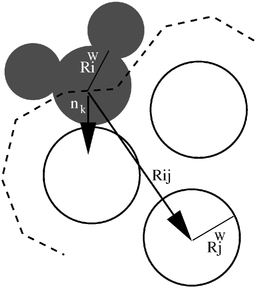
Figure 1:

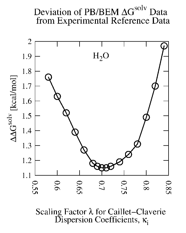
Figure 2:

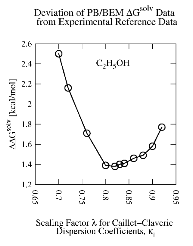
Figure 3:

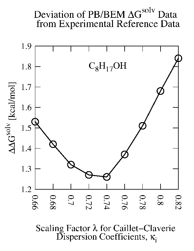
Figure 4:

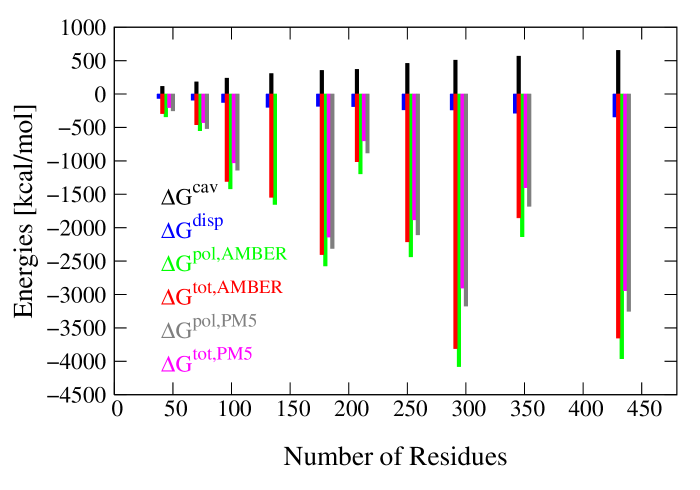
Figure 5:

References

- 1 Jorgensen, W. L.; Chandrasekhar, J.; Madura, J. D.; Impey, R. W.; Klein, M. L. J. Chem. Phys. 1983, 79, 926-935.
- 2 Berendsen, H. J. C.; Postma, J. P. M.; van Gunsteren, W. F.; Hermans, J. Intermolecular Forces; Reidel Publishing Company: Dordrecht, the Netherlands, 1981.
- 3 Ren, P.; Ponder, J. W. J. Phys. Chem. B 2003, 107, 5933-5947.
- 4 Tomasi, J.; Mennucci, B.; Cammi, R. Chem. Rev. 2005, 105, 2999-3094.
- 5 Rinaldi, D.; Ruiz-López, M. F., Rivail, J. L. J. Chem. Phys. 1983, 78, 834.
- 6 Roux, B.; Simonson, T. Biophys. Chem. 1999, 78, 1-20.
- 7 Ooi, T.; Oobatake, M.; Nemethy, G.; and Scheraga, H.A. Proc. Natl. Acad. Sci. USA 1987, 84, 3086–3090.
- 8 Cramer, C. J.; Truhlar, D. G. Chem. Rev. 1999, 99, 2161.
- 9 Still, W. C.; Tempczyk, A.; Hawley, R. C.; Hendrickson, T. J. Am. Chem. Soc. 1990, 112, 6127-6129.
- 10 Onufriev, A.; Bashford, D.; Case, D. A. J. Phys. Chem. B 2000, 104, 3712-3720.
- 11 Feig, M.; Onufriev, A.; Lee, M. S.; Im, W.; Case, D. A.; Brooks III, C. L. J. Phys. Chem. 1996, 100, 1578-1599.
- 12 Schaefer, M.; Karplus, M. J. Phys. Chem. 1996, 100, 1578-1599.
- 13 Warwicker, J.; Watson, H. C. J. Mol. Biol. 1982, 157, 671-679.
- 14 Honig, B.; Nicholls, A. Science 1995, 268, 1144-1149.
- 15 Luo, R.; David, L.; Gilson, M. K. J. Comput. Chem. 2002, 23, 1244-1253.
- 16 Baker, N. A.; Sept, D.; Joseph; S.; Holst, M. J.; McCammon, J. A. Proc. Natl. Acad. Sci. USA 2001, 98, 10037-10041.
- 17 Bashford, D.; Karplus, M. Biochemistry-US 1990, 29, 10219-10225.
- 18 Tironi, I.; Sperb, R.; Smith, P. E.; van Gunsteren, W. F. J. Chem. Phys. 1995, 102, 5451-5459.
- 19 Zauhar, R. J.; Morgan, R. S. J. Mol. Biol. 1985, 186, 815-820.
- 20 Juffer, A. H.; Botta, E. F. F.; van Keulen, B. A. M.; van der Ploeg, A.; Berendsen, H. J. C. J. Comput. Phys. 1991, 97, 144-171.
- 21 Mohan, V.; Davis, M. E.; McCammon, J. A.; Pettitt, B. M. J. Phys. Chem. 1992, 96, 6428-6431.
- 22 Kar, P.; Wei, Y.; Hansmann, U. H. E.; Höfinger, S. J. Comput. Chem. 2007, in press.
- 23 Zacharias, M. J. Phys. Chem. A 2003, 107, 3000-3004.
- 24 Pitera, J. W.; van Gunsteren, W. F. J. Am. Chem. Soc. 2001, 123, 3163-3164.
- 25 Simonson, T.; Brunger, A. T. J. Phys. Chem. 1994, 98, 4683-4694.
- 26 Su, Y.; Gallicchio, E. Biophys. Chem. 2004, 109, 251-260.
- 27 Wagoner, J. A.; Baker, N. A. Proc. Natl. Acad. Sci. USA 2006, 103, 8331-8336.
- 28 Gallicchio, E.; Levy, R. M. J. Comput. Chem. 2004, 25, 479-499.
- 29 Gallicchio, E.; Zhang, L. Y.; Levy, R. M. J. Comput. Chem. 2002, 23, 517-529.
- 30 Levy, R. M.; Zhang, L. Y.; Gallicchio, E.; Felts, A. K. J. Am. Chem. Soc. 2003, 125, 9523-9530.
- 31 Gallicchio, E.; Kubo, M. M.; Levy, R. M. J. Phys. Chem. B 2000, 104, 6271-6285.
- 32 Reiss, H.; Frisch, H. L.; Lebowitz, J. L. J. Chem. Phys. 1959, 31, 369-380.
- 33 Pierotti, R. A. Chem. Rev. 1976, 76, 717-726.
- 34 Höfinger, S.; Zerbetto, F. Chem. Soc. Rev. 2005, 34, 1012-1020.
- 35 Mahajan, R.; Kranzlmüller, D.; Volkert, J.; Hansmann, U. H. E.; Höfinger, S. Phys. Chem. Chem. Phys. 2006, 8, 5515-5521.
- 36 Case, D. A.; Cheatham, T. E.; Darden, T.; Gohlke, H.; Luo, R.; Merz Jr., K. M.; Onuvriev, A.; Simmerling, C.; Wang, B.; Woods, R. http://amber.scripps.edu J. Comput. Chem. 2005, 26, 1668-1688.
- 37 Mongan, J.; Simmerling, C.; McCammon, J. A.; Case, D. A.; Onuvriev, A. , J. Chem. Theory Comput. 2007, 3, 156-169.
- 38 Curutchet, C.; Orozco, M.; Luque, F. J.; Mennucci, B.; Tomasi, J. J. Comput. Chem. 2006, 27, 1769-1780.
- 39 Caillet, J.; Claverie, P. Acta Cryst. A 1975, 31, 448-461.
- 40 Claverie, P. in Intermolecular Interactions: From Diatomic to Biopolymers 1978, Wiley, New York, 69.
- 41 Floris, F. M.; Tomasi, J.; Pascual Ahuir, J. L. J. Comput. Chem. 1991, 12, 784-791.
- 42 Choudhury, N.; Pettitt, B. M. J. Am. Chem. Soc. 2005, 127, 3556-3567.
- 43 Choudhury, N.; Pettitt, B. M. in Modelling Molecular Structure and Reactivity in Biological Systems 2006, RSC Publishing, Cambridge UK, 49.
- 44 Choudhury, N.; Pettitt, B. M. J. Am. Chem. Soc. 2007, 129, 4847-4852.
- 45 Zhou, R.; Huang, X.; Margulis, C. J.; Berne, B. J. Science 2004, 305, 1605-1609.
- 46 Anikin, N. A.; Anisimov, V. M.; Bugaenko, V. L.; Bobrikov, V. V.; Andreyev, A. M. J. Chem. Phys., 2005, 121, 1266-1270.
- 47 Klamt, A.; Schürmann, G. J. Chem. Soc. Perk. T 2, 1993, 799
- 48 Connolly, M. L. http://www.netsci.org/Science/Compchem/feature14e.html J. Am. Chem. Soc., 1985, 107, 1118.
- 49 Höfinger, S. J. Comput. Chem., 2005, 26, 1148-1154.
- 50 Frisch, M. J.; Trucks, G. W.; Schlegel, H. B.; Scuseria, G. E.; Robb, M. A.; Cheeseman, J. R.; Zakrzewski, V. G.; Montgomery, J. A.; Stratmann, R. E.; Burant, J. C.; Dapprich, S.; Millam, J. A.; Daniels, A. D.; Kudin, K. N.; Strain, M. C.; Farkas, O.; Tomasi, J.; Barone, V.; Cossi, M.; Menucci, B.; Pomelli, C.; Adamo, C.; Clifford, S.; Ochterski, J.; Petersson, G. A.; Ayala, P. Y.; Cui, Q.; Morokuma, K.; Malick, D. K.; Rabuck, A. D.; Raghavachari, K.; Foresman, J. B.; Cioslowski, J.; Ortiz, J. V.; Stefanov, B. B.; Liu, A.; Liashenko, A.; Piskorz, P.; Komaromi, I.; Gomperts, R.; Martin, R. L.; Fox, D. J.; Keith, T.; Al-Laham, M. A.; Peng, C. Y.; Nanayakkara, A.; Gonzalez, C.; Challacombe, M.; Gill, P. M. W.; Johnson, B. G.; Chen, W.; Wong, M. W.; Andres, J. L.; Head-Gordon, M.; Replogle, E. S.; Pople, J. A. Gaussian Inc. Pittsburgh, PA, GAUSSIAN 98, Rev A.7, 1998
- 51 Vorobjev, Y. N.; Hermans, J. Biophys. J., 1997, 73, 722.
- 52 Chang, J.; Lenhoff, A. M.; Sandler, S. I. J. Phys. Chem. B 2007, 111, 2098-2106.
- 53 Frisch, M. J.; Trucks, G. W.; Schlegel, H. B.; Scuseria, G. E.; Robb, M. A.; Cheeseman, J. R.; Montgomery Jr., J. A.; Vreven, T.; Kudin, K. N.; Burant, J. C.; Millam, J. M.; Iyengar, S. S.; Tomasi, J.; Barone, V.; Mennucci, B.; Cossi, M.; Scalmani, G.; Rega, N.; Petersson, G. A.; Nakatsuji, H.; Hada, M.; Ehara, M.; Toyota, K.; Fukuda, R.; Hasegawa, J.; Ishida, M.; Nakajima, T.; Honda, Y.; Kitao, O.; Nakai, H.; Klene, M.; Li, X.; Knox, J.E.; Hratchian, H. P.; Cross, J. B.; Bakken, V.; Adamo, C.; Jaramillo, J.; Gomperts, R.; Stratmann, R. E.; Yazyev, O.; Austin, A. J.; Cammi, R.; Pomelli, C.; Ochterski, J. W.; Ayala, P. Y.; Morokuma, K.; Voth, G. A.; Salvador, P.; Dannenberg, J. J.; Zakrzewski, V. G.; Dapprich, S.; Daniels, A. D.; Strain, M. C.; Farkas, O.; Malick, D. K.; Rabuck, A. D.; Raghavachari, K.; Foresman, J. B.; Ortiz, J. V.; Cui, Q.; Baboul, A. G.; Clifford, S.; Cioslowski, J.; Stefanov, B. B.; Liu, G.; Liashenko, A.; Piskorz, P.; Komaromi, I.; Martin, R. L.; Fox, D. J.; Keith, T.; Al-Laham, M. A.; Peng, C. Y.; Nanayakkara, A.; Challacombe, M.; Gill, P. M. W.; Johnson, B.; Chen, W.; Wong, M. W.; Gonzalez, C.; Pople, J. A. Gaussian Inc. Wallingford, CT, GAUSSIAN 03, Rev B.05, 2004
- 54 Li, J.; Zhu, T.; Hawkins, G. D.; Winget, P. Liotard, D. A.; Cramer, C. J.; Truhlar, D. G. Theor. Chem. Acc., 1999, 103, 9-63.
- 55 Cornell, W. D.; Cieplak, P.; Bayly, C. I.; Gould, I. R.; Merz, K. M.; Ferguson, D. M.; Spellmeyer, D.; Fox, T.; Caldwell, J. W.; Kollman, P. A. J. Am. Chem. Soc., 1995, 117, 5179.
- 56 Berman, H. M.; Westbrook, J.; Feng, Z.; Gilliland, G.; Bhat, T. N.; Weissig, H.; Shindyalov, I. N.; Bourne, P. E. Nucleic Acids Res., 2000, 28, 235.
-
57
Akiyama, Y.; Onizuka, K.; Noguchi, T.; Ando, M.
Proc. 9th Genome Informatics Workshop (GIW’98),
Universal Academy Press, 1998, ISBN 4-946443-52-5, 131-140
http://mbs.cbrc.jp/pdbreprdb-cgi/reprdb_menu.pl - 58 Kar, P.; Wei, Y.; Hansmann, U. H. E.; Höfinger, S. Publication Series of the John von Neumann Institute for Computing, 2006, 34, 161-164.
- 59 Stewart, J. J. P. J. Mol. Model., 2004, 10, 6-12.
- 60 White, C. A.; Head-Gordon, M. J. Chem. Phys., 1994, 101, 6593.
- 61 Shirts, M. R.; Pande, V. S. J. Chem. Phys., 2005, 122, 134508.
- 62 MacCallum, J. L.; Tieleman, D. T. J. Comput. Chem., 2003, 24, 1930-1935.
- 63 Becke, A. D. J. Chem. Phys., 1997, 107, 8554.
- 64 Sadlej, A. J. Theor. Chim. Acta, 1991, 79, 123.
- 65 Höfinger, S.; Zerbetto, F. Theor. Chem. Acc., 2004, 112, 240.