The multiple quasar Q2237+0305 under a microlensing caustic

We use the high magnification event seen in the 1999 OGLE campaign light curve of image C of the quadruply imaged gravitational lens Q2237+0305 to study the structure of the quasar engine. We have obtained g’- and r’-band photometry at the Apache Point Observatory 3.5m telescope where we find that the event has a smaller amplitude in the r’-band than in the g’- and OGLE V-bands. By comparing the light curves with microlensing simulations we obtain constraints on the sizes of the quasar regions contributing to the g’- and r’-band flux. Assuming that most of the surface mass density in the central kiloparsec of the lensing galaxy is due to stars and by modeling the source with a Gaussian profile, we obtain for the Gaussian width $1.20\times 10^{15}\sqrt{{M}/{0.1M_{\odot}}}\leavevmode\nobreak\ cm\lesssim\sigma_{g^{\prime}}\lesssim 7.96\times 10^{15}\sqrt{{M}/{0.1M_{\odot}}}\leavevmode\nobreak\ cm$, where M is the mean microlensing mass, and a ratio $\sigma_{r^{\prime}}/\sigma_{g^{\prime}}=1.25^{+0.45}_{-0.15}$. With the limits on the velocity of the lensing galaxy from Gil-Merino et al. (2005) as our only prior, we obtain $0.60\times 10^{15}\sqrt{{M}/{0.1M_{\odot}}}\leavevmode\nobreak\ cm\lesssim\sigma_{g^{\prime}}\lesssim 1.57\times 10^{15}\sqrt{{M}/{0.1M_{\odot}}}\leavevmode\nobreak\ cm$ and a ratio $\sigma_{r^{\prime}}/\sigma_{g^{\prime}}=1.45^{+0.90}_{-0.25}$ (all values at 68 percent confidence). Additionally, from our microlensing simulations we find that, during the chromatic microlensing event observed, the continuum emitting region of the quasar crossed a caustic at $\geq 72$ percent confidence.

1 Introduction

One of the best studied quasar lensing systems yet is Q2237+0305. This quasar was discovered by the Center for Astrophysics (CfA) redshift survey Huchra et al. (1985). The system is made up of a barred spiral galaxy (z=0.0394) and four images of a quasar at a redshift of z=1.695 that appear in a nearly symmetric configuration around the core of the spiral galaxy at a distance of approximately 1” from the center.

Q2237+0305 is an ideal system to study quasar microlensing. At the position of the quasar images the optical depth due to microlensing by the stars is high Kayser et al. (1986); Kayser & Refsdal (1989); Wambsganss et al. (1990). Furthermore the expected time-delay between the images of this quasar is of the order of a day or less Schneider et al. (1988); Rix et al. (1992); Wambsganss & Paczynski (1994). As microlensing events for this system are of the order of months or years, it is easy to distinguish intrinsic variability from microlensing. Another big advantage is the fact that the quasar is $\sim$10 times farther from us than the lensing galaxy. This leads to a large projected velocity of the stars in the source plane and thus a short timescale of caustic events. Not long after its discovery in 1985, Irwin et al. (1989) observed the first microlensing signature in this quasar.

The quasar has been monitored for almost two decades by different surveys (e.g., Corrigan et al. 1991; Pen et al. 1993; Ostensen et al. 1996; Alcalde et al. 2002; Schmidt et al. 2002). The one that has the longest and best sampled data is that of the Optical Gravitational Lensing Experiment (OGLE) team Woźniak et al. (2000); Udalski et al. (2006). They have monitored Q2237+0305 since 1997 delivering the most complete light curves for this system in which many microlensing events can be seen. These data have been used for various studies on the system: Wyithe et al. (2000a, b, d, e, f); Yonehara (2001); Shalyapin et al. (2002) and Kochanek (2004) used this data together with microlensing simulations not only to obtain limits on the properties of the quasar such as size and transversal velocity, but also on the mass of the microlensing objects.

The OGLE team has monitored this quasar with a single V band filter. However, Wambsganss & Paczynski (1991) showed that color variations should be seen in quasar microlensing events and how they would provide additional information on the background source. We know from thermal accretion disk models that emission in the central regions of a quasar should be bluer than in the outer regions (e.g., Shakura & Sunyaev 1973). As an approximation we can assume the central engine of the quasar to be of the order of 1000 Schwarzschild radii:

$$R_{\rm ad}=1000\times r_{s}=2.8\times 10^{16}\left(\frac{M_{\rm BH}}{10^{8}M_{\odot}}\right){\rm cm}$$ (1)

where $r_{s}$ is the Schwarzschild radius, $R_{\rm ad}$ is the radius of the accretion disk and $M_{\rm BH}$ is the mass of the black hole. We can compare this value with the Einstein Radius ($R_{E}$) - the length scale in quasar microlensing - which can be given in the source plane by Schneider et al. (1992):

$$R_{E}=\sqrt{\frac{4GM}{c^{2}}\frac{D_{s}D_{ls}}{D_{l}}}=5.68\times 10^{16}\sqrt{\frac{M}{0.1M_{\odot}}}{\rm cm}$$ (2)

where we have replaced the values of the distances $D_{l}$, $D_{s}$ and $D_{ls}$ to the ones corresponding to Q2237+0305. The accretion disk scales are thus comparable to those of the Einstein rings of stars in the lensing galaxy. This shows that differential magnification of the different emission regions of the quasar can be observed.

Some multi-band observations of this system have been carried out Corrigan et al. (1991); Vakulik et al. (1997, 2004); Koptelova et al. (2005), however most of them have either large gaps between the observations, or no obvious microlensing event.

A very interesting event, that has been one of the bases for predictions Wyithe et al. (2000b) and study Yonehara (2001); Shalyapin et al. (2002); Vakulik et al. (2004), is the high magnification event of image C in the year 1999 as observed by OGLE.

In this paper we present data of this particular event obtained in two filters at Apache Point Observatory (APO). We analyze the event using both the OGLE light curve and the APO data and study the implications for the size of the quasar emission region using microlensing simulations. We use a flat cosmology with $\Omega_{m}=0.3$ and $H_{0}=70\leavevmode\nobreak\ km\leavevmode\nobreak\ s^{-1}Mpc^{-1}$.

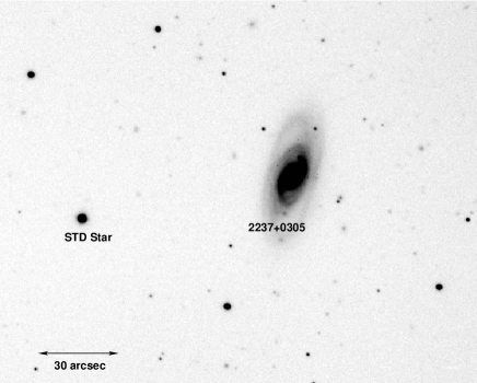
Figure 1: APO g’ image of the quasar system Q2237+0305.

2 Apache Point observatory Data, Observations & Data reduction

For this study we use two different datasets. The first one is that of the OGLE team light curves for this quasar Woźniak et al. (2000); Udalski et al. (2006) for which we select the data between Julian days 2451290 (April 21, 1999) and 2451539 (December 26, 1999), which comprises 83 data points. The result is a dense light curve for the event we analyze. The second data set is APO two-band monitoring data for Q2237+0305. We selected the nights between May 17 1999 (Julian day: 24511316) and January 8 2000 (Julian day: 24511551) which also track the event, comprising 8 nights with data points.

The APO data were taken with the 3.5 m telescope at Apache Point Observatory using the Seaver Prototype Imaging camera (SPIcam) in both the SDSS g’ and r’ filters. The SPIcam has a 2048$\times$2048 pixels CCD and a minimum pixel scale of 0.141 ”/pixel, however, for the observations we use, the pixels were binned to 0.282 ”/pixel.

2.1 Standard CCD Reduction

For the standard CCD reduction we use a combination of the astronomical image reduction software package iraf and idl data language. We apply bias correction, create one master flat-field image for each night and each filter and calibrate the science frames with these. Cosmic rays are eliminated from the science frames using median filtering outside the sources.

In order to remove the remaining cosmic rays and imperfections of the CCD as well as to improve the signal to noise ratio of the images, we combine the frames corresponding to the same night, excluding those with asymmetric point spread functions (PSFs). In the end we obtain a clean high quality image for each night in g’ and r’ filters.

2.2 Photometry

The photometry for this system is made difficult because the quasar images are seen through the core of the lensing galaxy. Our first attempt, following the procedure as in Woźniak et al. (2000), was to use an image subtraction method Alard & Lupton (1998). However our field of view lacks the high number of bright stars required in order to run a successful correlation and PSF characterization for the procedure. This is why we use galfit Peng et al. (2002) instead. galfit is a galaxy/point source fitting algorithm that fits 2-D parameterized image components directly to the images.

2.2.1 galfit model

For the galaxy we use the model shown by Schmidt (1996) (see also Trott & Webster 2002) from HST F7815LP band data, in which the lensing galaxy is parameterized with a de Vaucouleurs profile for the bulge and an exponential profile for the disk. The bulge’s de Vaucouleurs profile is constrained to a 4.1” (3.1 kpc) scale length, a 0.31 ellipticity and a 77^∘ position angle. For the exponential profile we use a 11.3” (8.6 kpc) scale length, a 0.5 ellipticity and a 77^∘ position angle. These profiles are constrained to have the exact same central position within the image and a fixed magnitude difference.

The quasar images are parameterized as point sources. The relative separation between them is fixed in the galfit code to the values obtained by Blanton et al. (1998) from UV data and the separation between the group of images and the center of the bulge is fixed to the values obtained with HST F7815LP filter data (HST proposal ID 3799): $\Delta_{RA}=-0.075^{\prime\prime}$ and $\Delta_{DEC}=0.937^{\prime\prime}$.

The PSF we use to convolve the different parameterizations is taken from the bright star (STD) shown in Fig. 1. After fitting the different profiles, the brightness of each component is measured. We run the galfit routine over each night in each one of the two bands available. The residuals from this fitting technique are low, usually of the order of 5 percent. In order to obtain error bars on the magnitude measurements, we create 500 Monte-Carlo realizations of the observed images and determine the measurement uncertainty from the scatter of the galfit results. The g’- and r’-band light curves for image C are shown in Fig. 2. The measurements for images A and C are given in Table 1. No reliable photometry is obtained for images B and D because they were too faint.

As shown in Fig. 2, the APO g’-band light curve shows a very similar behaviour to the OGLE V-band light curve, however, the APO r’-band light curve shows a lower amplitude at the brightness peak. Thus, the resultant g’-r’ color curve, does not appear flat but shows a chromatic variation during the microlensing event.

Table 1: APO light curves for quasar images A and C. Magnitudes are shown relative to the value of the last data point of image C in the g’ filter.

Julian Day	A				C
+2451000	g’		r’		g’		r’		FWHM
	$\Delta$ [mag]	err [mag]	$\Delta$ [mag]	err [mag]	$\Delta$ [mag]	err [mag]	$\Delta$ [mag]	err [mag]	[arcsec]
1315	-0.822	0.016	-0.675	0.012	-0.533	0.016	-0.381	0.013	1.6
1334	-0.826	0.056	-0.680	0.021	-0.554	0.056	-0.393	0.021	1.4
1373	-0.925	0.017	-0.729	0.013	-0.672	0.017	-0.445	0.013	1.2
1385	-0.971	0.017	-0.782	0.015	-0.635	0.017	-0.411	0.015	1.0
1400	-0.912	0.019	-0.757	0.014	-0.487	0.019	-0.298	0.014	1.1
1531	-1.148	0.024	-0.887	0.015	-0.013	0.026	0.067	0.015	1.1
1541	-1.158	0.015	-0.909	0.015	-0.037	0.016	0.016	0.018	1.1
1551	-1.137	0.018	-0.916	0.014	0.000	0.024	0.094	0.015	1.2

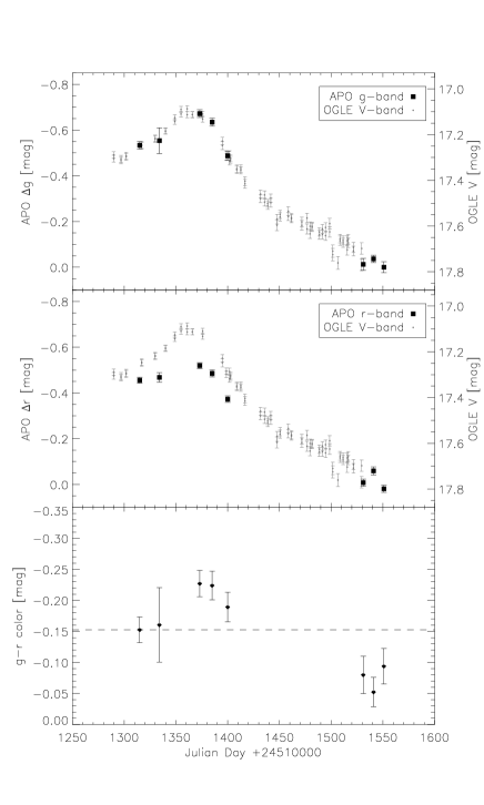
Figure 2: Top panel: Black squares show the APO g’-band light curve (relative to the faintest data point) of the high magnification event seen in image C of Q2237+0305 in 1999. For comparison, in light gray, the OGLE V-band light curve sampling this event is shown. Middle panel: APO r’-band light curve for the event (black squares) and the OGLE V-band light curve plotted in light gray. Bottom panel: APO g’-r’ color curve. The dashed line is shown to guide the eye.

3 Microlensing Simulations

In order to compare the observed data with simulations we generate source-plane magnification patterns for quasar images C and B using the inverse ray shooting method Wambsganss et al. (1990); Wambsganss (1999). We assume identical masses for all the microlenses distributed in the lens plane (the results do not depend on the mass distribution of the microlenses Lewis & Irwin (1996)). Approximately $10^{11}$ rays are shot, deflected in the lens plane and collected in a 10,000 by 10,000 pixels (equivalent to 50 Einstein radii by 50 Einstein radii) array in the source plane. The values of surface density $\kappa$ and shear $\gamma$ are taken from Schmidt et al. (1998) (Table 2). The convergence $\kappa$ is separated into a compact matter distribution $\kappa_{\star}$ and a smooth matter distribution $\kappa_{c}$. Even though we explore different stellar fractions, as the quasar images are located within the central kiloparsec of the lensing galaxy, we focus our work mainly on the $\frac{\kappa_{\star}}{\kappa}=1$ stellar fraction.

Table 2: Local macro-lensing parameters for quasar images B and C from Schmidt et al. (1998). $\kappa$ is the scaled surface density, $\gamma$ is the shear, $\mu_{tot}$ is the total magnification.

Image	$\kappa$	$\gamma$	$\mu_{tot}$
B	0.36	0.42	4.29
C	0.69	0.71	2.45

As shown in Sect. 1, in quasar microlensing the source size is an important parameter because it is comparable with typical caustic scales (e.g, Kayser et al. 1986). In order to study a sample of different source sizes, the raw magnification patterns are convolved with a set of profiles. Mortonson et al. (2005) showed that microlensing fluctuations are relatively insensitive to the source shape, so it is of little consequence whether we choose a standard model accretion disk Shakura & Sunyaev (1973) or a Gaussian profile. For simplicity we choose a Gaussian profile for the surface brightness where the extent of the source is described by the variance $\sigma$. The full width half maximum (FWHM) is defined as 2.35$\sigma$.

We vary the FWHM of a Gaussian profile from 2 to 120 pixels (which corresponds to 0.01 $E_{R}$ and 0.60 $E_{R}$, respectively) for quasar image B and from 2 to 216 pixels (which corresponds to 0.01 $E_{R}$ and 1.08 $E_{R}$, respectively) for quasar image C (the additional magnification patterns for image C are used for the color curve fitting explained in Section 5). For patterns below 12 pixels the step size is 2 pixels, and for patterns above 12 pixels the step size is 4 pixels. We find that this linear sampling gives more accurate results when interpolating compared to a logarithmic sampling.

For a specific convolved pattern we can now extract light curves. By defining a track (path of the source in the source plane magnification pattern) with a starting point, direction and velocity, we extract the pixel counts in the positions of the pattern defined by this track using bi-linear interpolation. The values are then scaled with the magnification values of Table 2 for each image and converted into magnitudes.

4 Light curve fitting

4.1 OGLE V light curve

Since quasars vary intrinsically, we need to separate this variation from microlensing. We therefore study the difference between two light curves extracted from microlensing patterns for different images to eliminate this effect and allow for an additional magnitude difference (the time delay is negligible, see Sect. 1).

Using the V band OGLE light curves sampling this event in both images C and B of the quasar Woźniak et al. (2000); Udalski et al. (2006) we construct the difference light curve C-B. Simulated light curves for each image are extracted using tracks over microlensing patterns created independently for each image and convolved with a Gaussian profile with the same size. By repeated light curve extraction with variation of the parameters, the best fit to these are obtained from the comparison with the OGLE C-B difference light curve. What is actually fitted are the parameters that define the track from which both light curves are obtained. This track is constrained to have identical direction and velocity in both the patterns C and B, but the starting point can be different among the different patterns. It is important to remark that the direction is set to be the same in both patterns, taking into consideration that the shear direction between images C and D is approximately perpendicular Witt & Mao (1994).

For the minimization method we use a Levenberg-Marquardt least squares routine in idl. This routine is a $\chi^{2}$-based minimization based upon MINPACK-1 Moré et al. (1980). As we are using 68 percent values for our errors, the $\chi^{2}$ is simply calculated as:

$$\chi^{2}=\sum_{i=0}^{DOF}\left(\frac{y_{i}-f(x_{i})}{\sigma^{err}_{i}}\right)^{2}$$ (3)

where DOF is the number of degrees of freedom, $y$ is the measured value, $x$ is the independent variable model and $\sigma^{err}$ is the one sigma error of the particular measurement. In the case in which we fit the OGLE data for this event, the number of degrees of freedom is 75. $y_{i}$ are the differences between the OGLE light curves for images C and B, $\sigma^{err}_{i}$ are the uncertainties measured by the OGLE team, $x_{i}$ are Julian days and $f(x_{i})$ are the difference between of the two light curves extracted from the source plane magnification patterns for images C and B convolved with an identical source profile. We also include a parameter which we call $m_{0}$ that accounts for the magnitude offset between the images.

As the size of each one of the convolved patterns is very large compared to the time scale of the chosen event (of the order of several hundred times), and considering the fact that it is relatively easy to find good fits because of the huge parameter space that such large patterns give, we need to determine a high number of tracks for each pattern. To obtain a statistical sample, we search for 10,000 tracks for each considered source size. The first guesses for each one of the tracks are distributed uniformly. However, during the fitting process the starting points of the tracks are constrained to stay within a square of 200 pixels sidelength around the random initial value in order to force a sampling of the whole pattern. After this minimization is done we have a track library containing 3$\times 10^{5}$ fitted tracks (10,000 tracks for 30 different source sizes with best-fitting velocity and magnitude offset).

4.2 APO Color Curve

Fig. 2 shows that the OGLE V-band and the APO g’-band light curves are very similar. Since the microlensing effect depends strongly on the source size, we assume, for simplicity, that the OGLE V-band continuum region is of similar size as that of the APO’s g’-band. Here we determine the ratio of the APO r’-band region and the g’-/OGLE V-band regions that follows from the color curve in Fig. 2.

While the parameters that define the tracks are fixed by the procedure shown in the previous section, the two parameters that influence the shape of the color curve in this step are the ratio between the sizes of the two regions and the intrinsic color g’-r’ of the quasar ($c_{0}$). These are the only parameters allowed to vary during this step. As before, we use the patterns convolved with Gaussian profiles up to 120 pixels FWHM for image C to obtain the g’-band light curve. To obtain the r’-band light curve we use the full set of patterns for image C. During the fitting process we interpolate the magnitude values of the extracted light curves in order to obtain continuous values for the source size ratio. After this second fitting procedure, the $\chi^{2}$ values of the track library are updated: $\chi^{2}=\chi_{OGLE}^{2}+\chi_{APO}^{2}$.

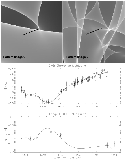
Figure 3: Example track for a 0.05 $E_{R}$ (10 pixel) FWHM g’-band source size and a source size ratio $\sigma_{r^{\prime}}/\sigma_{g^{\prime}}=1.48$. In the top panels the fitted track is shown in a $1.0E_{R}\times 1.0E_{R}$ section of the microlensing patterns. In the middle panel we plot the fitted difference light curve (solid line) and the observed OGLE difference light curve. In the lower panel the best-fitting color curve (solid line) and the APO g’-r’ color curve are shown.

5 Considerations

5.1 Degeneracies

As source size and microlens mass are degenerate, we express the size values in Einstein radii or scaled by a stellar mass as shown in equation (2). Another important degeneracy is the one between the size of the source and the transversal velocity we fit. If we fix the path velocity of a source and increase the size of it, its light curve will get broader. Conversely, if we fix a source size and decrease the velocity, the light curve will also become broader because it takes longer time for the source to cross the magnification region.

5.2 Velocity considerations

The velocity one measures for a microlensing event is composed of velocities of the observer, the lenses and the source. The Earth’s motion relative to the microwave background is likely to be almost parallel to the direction of the quasar Q2237+0305 Witt & Mao (1994) so the velocity of the observer is negligible compared to the other velocity values. We assume the physical velocities of the lens and the source of the same order of magnitude, thus, the main contribution to the total velocity is the velocity of the lens due to the fact that the source velocity is weighted by $\sim$3.5 percent compared to the lens velocity (Kayser et al. 1986).

The velocity of the lens has two components: one of the bulk velocity of the galaxy $v_{b}$ and the velocity dispersion of the stars in the galaxy (microlenses) $v_{\mu}$. Since the time span of the event that we fit is $\sim$200 days, the significance of individual stellar motions in the fitting should be fairly low. Moreover, Kundic & Wambsganss (1993) and Wambsganss & Kundic (1995) show that, in a statistical sense, the overall effect of the individual stellar motions can be approximated by an artificially increased velocity (a factor $\approx 1.3$) of the source across the pattern.

The scale we use for fitting the velocity is pixels per Julian day. Using equation (2) we can see that this turns into:

$$1\leavevmode\nobreak\ \frac{pix}{jd}\leavevmode\nobreak\ =\leavevmode\nobreak\ 0.005\leavevmode\nobreak\ \frac{E_{R}}{jd}=32870\sqrt{\frac{M}{0.1M_{\odot}}}\frac{km}{s}$$ (4)

in the source plane. Using the appropriate velocity scaling (Kayser et al. 1986), we find: 1 $\frac{pix}{jd}$ $\sim$ 3000 $\frac{km}{s}$ in the lens plane.

5.3 Size Considerations

In a standard thin accretion disk model of a quasar the black hole is surrounded by a thermally radiating accretion disk Shakura & Sunyaev (1973). Kochanek et al. (2006) show that the radii $R_{\lambda}$ where radiation with wavelength $\lambda$ is emitted scale as $\lambda^{\frac{4}{3}}$. Thus:

$$f=\frac{R_{\lambda_{1}}}{R_{\lambda_{2}}}=\left(\frac{\lambda_{1}}{\lambda_{2}}\right)^{\frac{4}{3}}.$$ (5)

For the observed data from APO, the transmission curve for the SPIcam g’ and r’ filters have central wavelengths of $\sim$4700Å and $\sim$6400Å, respectively. Using these values and equation (5) we obtain a predicted thin-disk ratio between the r’- and g’-band source sizes of $\sim 1.5$.

6 Statistical Analysis

There are different ways to approach quasar microlensing studies. It can be by analytical model fitting of the light curves (e.g., Yonehara 2001), studying the structure function (e.g., Lewis & Irwin 1996), doing statistics of parameter variations over time intervals (e.g., Schmidt & Wambsganss 1998; Wambsganss et al. 2000; Gil-Merino et al. 2005), obtaining probability distributions with light curve derivatives (e.g., Wyithe et al. 2000c) or Bayesian analysis (e.g., Kochanek 2004). Similar to Kochanek (2004), we construct a probability distribution for the quantities of interest (V/g’-band source size, source size ratio and transversal velocity) from our track library.

Each one of our tracks is a fit to the light and color curves and therefore has a $\chi^{2}$ value attached to it. We therefore infer information from the whole ensemble of models: the track library. Using the standard approach for ensemble analysis (e.g., Sambridge 1999), we assign a likelihood estimator to each track $t_{i}$: $p(t_{i})\propto\exp({\frac{\chi^{2}(t_{i})}{2}})$. Using this likelihood estimator the statistical weight for each track can be written as:

$$w(t_{i})=\frac{p(t_{i})}{n(t_{i})}$$ (6)

where $w(t_{i})$, $p(t_{i})$ and $n(t_{i})$ are, respectively, the weight, the likelihood obtained from the $\chi^{2}$ and the density parameter for each track $t_{i}$. The density parameter describes the local track density in a multidimensional grid in which each dimension corresponds to a parameter of interest. The density is normalized so that the sum of all the density parameters in the grid equals one. By summing over the statistical weights, we can calculate probability distribution histograms for all the parameters of interest.

Gil-Merino et al. (2005) (from now on G-M05) found an upper limit of 625 $\frac{km}{s}$ (90 percent confidence) on the effective transverse velocity of the lensing galaxy in Q2237+0305. They performed microlensing simulations assuming microlenses with $M=0.1M_{\odot}$ for three different source sizes yielding similar results. We use their probability distribution for the velocity obtained with the largest source size value (Fig. 5 in G-M05) in a further analysis step, where we factor it into our own probability distributions by importance sampling. In other words, we scale the probability of finding a track based on the G-M05 prior, and then reobtain the best-fitting value for each parameter and confidence regions.

7 Results and Discussion

Table 3: Results and confidence limits for g’-band source size, ratio between r’- and g’-band source size and transverse velocity (projected to the lens plane).

No Prior					With G-M05 Prior
Source Size $\sigma_{g^{\prime}}$		Ratio	Velocity (*)		Source Size $\sigma_{g^{\prime}}$		Ratio	Velocity
$\times 10^{-2}$ $R_{E}$	$\sqrt{\frac{M}{0.1M_{\odot}}}$	$\frac{\sigma_{r^{\prime}}}{\sigma_{g^{\prime}}}$	$\sqrt{\frac{M}{0.1M_{\odot}}}$		$\times 10^{-2}$ $R_{E}$	$\sqrt{\frac{M}{0.1M_{\odot}}}$	$\frac{\sigma_{r^{\prime}}}{\sigma_{g^{\prime}}}$	$\sqrt{\frac{M}{0.1M_{\odot}}}$
	$\times 10^{15}$[cm]		[km/s]			$\times 10^{15}$[cm]		[km/s]
$8.10^{+5.90}_{-5.99}$	$4.60^{+3.36}_{-3.40}$	$1.25^{+0.45}_{-0.15}$	$2930$		$2.34^{+0.43}_{-1.28}$	$1.33^{+0.24}_{-0.73}$	$1.45^{+0.90}_{-0.25}$	$682^{+227}_{-379}$

(*) The velocity obtained without the G-M05 prior is shown without error bars as we do not obtain limits for it.

As described in the previous section, we obtain limits on the source size and transverse velocity from two sets of probability distributions. The first corresponds to the parameters obtained without using any prior, and a second one in which we apply the G-M05 prior on the velocity of the lens galaxy. For each probability distribution of a particular parameter we select the 68 percent confidence levels. This is done by making horizontal cuts starting from the highest probability and screening down until 68 percent of the cumulative probability is reached. The distribution, the best-fitting values (or the average of the 68 percent confidence region where no single best-fitting solution is found) and the 68 percent confidence limits for the relevant parameters are shown in Fig. 4 and Table 3. After applying the G-M05 prior only $\sim$1000 tracks carry 99 percent of the statistical weight. This makes the probability histogram for the source ratio sparsely populated for $\sigma_{r^{\prime}}/\sigma_{g^{\prime}}>2$. Therefore, we require at least 70 of these 1000 tracks to be part of each bin in the histogram.

Without any velocity prior (see Fig. 4), we have more fast tracks than slow tracks. No limit on the transversal velocity can be determined. This mostly is due to the degeneracy between source size and transverse velocity (see Section 5.1). Using the G-M05 prior, we obtain a best-fitting velocity of $682^{+227}_{-379}\sqrt{\frac{M}{0.1M_{\odot}}}km/s$ (projected into the lens plane). Note, however, that the distribution shows a longer tail towards the higher velocities when compared to the G-M05 probability distribution because the steepness of the event fitted prefers fast tracks or small source sizes.

The average Gaussian width we obtain on the OGLE V/APO g’ source size without setting the velocity prior is $\sigma_{g^{\prime}}=8.10^{+5.90}_{-5.99}\times 10^{-2}R_{E}$ or $4.60^{+3.36}_{-3.40}\times 10^{15}\sqrt{\frac{M}{0.1M_{\odot}}}cm$. These limits agree with those obtained by Yonehara (2001) and Kochanek (2004) (who used a logarithmic prior on the transversal velocity). When we impose the velocity constraints of G-M05 we obtain an OGLE V/APO g’ source size with a Gaussian width of $\sigma_{g^{\prime}}=2.34^{+0.43}_{-1.28}\times 10^{-2}R_{E}$ which is equivalent to $1.33^{+0.24}_{-0.73}\times 10^{15}\sqrt{\frac{M}{0.1M_{\odot}}}cm$. This makes the upper limit tighter by a factor of five compared to the previous result, placing it just below the 68 percent confidence limit obtained by Kochanek (2004), very close to their resolution limit. For $m_{0}$ we obtain $-1.75\lesssim m_{0}\lesssim 0.25$ without and $-0.75\lesssim m_{0}\lesssim 1.25$ with the G-M05 prior, respectively (see Section 4.1).

The source size ratio between the r’- and g’-band emitting regions of the quasar is $\sigma_{r^{\prime}}/\sigma_{g^{\prime}}=1.25^{+0.45}_{-0.15}$ without, and $\sigma_{r^{\prime}}/\sigma_{g^{\prime}}=1.45^{+0.90}_{-0.25}$ with the G-M05 prior, respectively, coupled with an intrinsic color parameter: $c_{0}=-0.18\pm 0.05$ in both cases (see Section 4.2). As shown in Fig. 4, both source size ratio distributions are similar. The measurements are close to the theoretical value (f$\sim$1.5) estimated in Section 5.3 from the Shakura & Sunyaev (1973) thermal profile.

For a long time there has been discussion on the nature of the image C event in year 1999 (e.g., Wyithe et al. 2000b; Yonehara 2001; Shalyapin et al. 2002; Kochanek 2004). Using different methods it was found that this event is likely to have been produced by the source passing near a cusp. We investigate this for the tracks in our library by computing the location of the caustics for each of the magnification patterns using the analytical method by Witt (1990, 1991) (combination of both ray shooting simulations and analytical caustics are shown in Wambsganss et al. 1992).

For each track we determine whether either the center, the center$\pm\sigma_{g^{\prime}}$ or the center$\pm\sigma_{r^{\prime}}$ of the source touches a caustic at any time. Our analysis agrees with the previous results when we use the OGLE light curve to fit for this event. However, to reproduce our APO color dataset, tracks that cross a caustic are favored (see Table 4). We find that a source with a radius as big as $\sigma_{r^{\prime}}$ touched a caustic with 97 percent and 94 percent of confidence without and with the G-M05 prior, respectively. Furthermore, the source, regardless of dimensions, crossed a caustic with a 75 percent and 72 percent of confidence without and with the G-M05 prior, respectively (i.e. the center of the source touched a caustic).

Table 4: Probabilites of the image C high magnification event being produced by the source crossing a caustic and of the g’ and r’-band region touching a caustic. The table shows the obtained values for the probability both using and not using the Gil-Merino et al. (2005) velocity prior.

No Prior			With G-M05 Prior
cross	g’	r’	cross	g’	r’
0.75	0.92	0.97	0.72	0.89	0.94

The probabilities of the source touching a caustic at different radii are bigger in the case in which we do not use the G-M05 prior as seen in detail in Table 4. This is due to the fact that a higher velocity makes a track cover more distance through the pattern and thus is more likely to encounter a caustic.

Figure 4: Probability histograms for g’ or V source size, r’/g’ source size ratio and transverse velocity (projected to the lens plane), respectively. The dotted line shows the best-fitting values (or average of the 68 percent confidence region if no single best-fitting value is found). The error bars describe the 68 percent confidence limits.

8 Conclusions

We present two band (g’ and r’) APO data covering the high magnification event seen in image C of the quadruple quasar Q2237+0305 in the year 1999. We find that the amplitude of the brightness peak is more pronounced in the g’-band than in the r’-band. This is also consistent with the observations by Vakulik et al. (2004) (see also the recent analysis by Koptelova et al. 2007).

By using this data together with the well known OGLE data Woźniak et al. (2000); Udalski et al. (2006) and combining it with microlensing simulations, we have been able to obtain limits on the size of regions of the quasar’s central engine emitting in these bands: Gaussian width $\sigma_{g^{\prime}}=4.60^{+3.36}_{-3.40}\times 10^{15}\sqrt{{M}/{0.1M_{\odot}}}$ cm and $\sigma_{r^{\prime}}/\sigma_{g^{\prime}}=1.25^{+0.45}_{-0.15}$.

Because of the degeneracy between source size and transverse velocity we use a prior on the velocity obtained from the work of Gil-Merino et al. (2005) in order to improve the results: Gaussian width $\sigma_{g^{\prime}}=1.33^{+0.24}_{-0.73}\times 10^{15}\sqrt{{M}/{0.1M_{\odot}}}$ cm and $\sigma_{r^{\prime}}/\sigma_{g^{\prime}}=1.45^{+0.90}_{-0.25}$. Both values for the ratio between the source sizes are close to the ratio obtained for a face-on Shakura & Sunyaev (1973) accretion disk (f$\sim$1.5). Recent studies (e.g., Poindexter et al. 2007; Morgan et al. 2007; Pooley et al. 2007) suggest microlensing yields a slightly bigger value for the ratio than that obtained analytically with the thin disk model (see Section 5.2), also in agreement with our results.

We also show that this event was probably produced by the source directly interacting with a caustic as we obtain probabilities of 97 percent and 94 percent that the r’-band emitting region touches a caustic without and with the G-M05 prior, respectively, and of 75 percent and 72 percent that the source center (regardless of size) crossed a caustic without and with the G-M05 prior, respectively.