Extinction properties of lensing galaxies

Abstract

Context. Observations of quasars shining through foreground galaxies, offer a way to probe the dust extinction curves of distant galaxies. Interesting objects for this study are found in strong gravitational lensing systems, where the foreground galaxies generate multiple images.

Aims. The reddening law of lensing galaxies is investigated by studying the colours of gravitationally-lensed quasars, and a handful of other quasars where a foreground galaxy is detected.

Methods. We compare the observed colours of quasars reported in the literature, with spectral templates reddened by different extinction laws and dust properties. The data consists of 21 quasar-galaxy systems, with a total of 48 images. The galaxies, which are both early- and late-type, have redshifts in the interval $z=\$$0.04-1.51$.

Results. We measure a difference in rest-frame $B-V$ between the quasar images we study, and quasars without resolved foreground galaxies. This difference in colour is indicative of significant dust extinction in the intervening galaxy. Good fits to standard extinction laws were found for 22 of the images, corresponding to 13 different galaxies. Our fits imply a wide range of possible values for the total-to-selective extinction ratio, $R_{V}$. The distribution was found to be broad with a weighted mode of $\bar{R}_{V}$=2.4 and a FWHM of $\Delta{R{{}_{V}}}$=2.7 ($\sigma_{R_{V}}\sim$ 1.1). Thus the bulk of the galaxies for which good reddening fits could be derived, have dust properties compatible with the Milky Way value ($R_{V}=3.1$).

1 Introduction

Measuring the reddening due to dust in galaxies, provides information on dust grains in the interstellar medium. It is in addition important for dimming corrections, when measuring cosmological distances using Type Ia supernovae, the most direct probe of the expansion history of the Universe.

It is often assumed that the wavelength dependence of extinction in distant galaxies is identical to the average in the Milky Way. However, there are indications that this is not always the case (e.g. Prévot et al. 1984; Calzetti et al. 2000). The purpose of this work is to examine the reddening relations in galaxies over a wide range of redshifts, to improve our understanding of galaxy dust properties.

For galaxies in which individual stars are resolved, dust extinction can be studied using the pair method. In this method, the galaxy extinction curve is determined by comparing the spectral energy distribution of reddened and non-reddened stars of the same spectral type and luminosity class (Massa et al. 1983). For more distant galaxies, other methods must be used, such as comparing the galaxy colours with a dust-free model (although this is subject to large model dependencies) (see e.g. Patil et al. 2007), determining the differential extinction of multiply-imaged quasars (e.g. Falco et al. 1999), or measuring the absolute extinction by foreground galaxies of quasars (Östman et al. 2006). There are problems using the method of differential extinction for multiply-imaged quasars. To obtain a unique $R_{V}$ value, one of the images must have negligible dust extinction when compared to the other, or the extinction curves must be similar along the two separate lines of sight. The potential problem of this limitation is discussed in McGough et al. (2005) and Elíasdóttir et al. (2006). If these conditions are not met, the $R_{V}$ value derived will be a function of the extinctions along the two lines of sight, and their $R_{V}$ values (see Eq. 6 in McGough et al. (2005)). In this paper, this restriction is circumvented by studying the individual colours of background quasar images in order to investigate the reddening by foreground galaxies. This is possible because of the fairly homogeneous spectral properties of quasars. The method is very similar to the one used in Östman et al. (2006), where the focus was on finding systems by matching the positions of quasars with galaxies. In this paper, the focus is on using systems found through gravitational lensing.

Studies of colours of Type Ia supernovae have also been used to constrain the dust properties of their host galaxies (e.g. Jõeveer 1983; Branch & Tammann 1992; Riess et al. 1996; Reindl et al. 2005; Guy et al. 2005). When the reddening correction has been optimised to minimise the scatter of the Type Ia supernova Hubble diagram, a quite different wavelength dependence of the extinction curve, when compared to the Milky Way, has been derived (e.g. Astier et al. 2006). It is unclear whether these findings indicate the presence of non-standard dust along the line of sight to supernovae, or if they point to a different source of the brightness-colour relation, perhaps intrinsic to supernovae themselves. We aim to establish if the reddening laws derived using supernovae are applicable to different astrophysical scenarios, such as quasars shining through galaxies.

In Sec. 2, different parameterisations of dust attenuation are discussed. The method for estimating the dust properties is presented in Sec. 3. The results and a discussion of the results are given in Sec. 4. Finally, we summarise and conclude in Sec. 5.

2 Dust extinction parameterisations

Extinction curves are often parameterised by the reddening parameter called the total-to-selective extinction ratio $R_{V}$, which is defined by

$$R_{V}\equiv\frac{A_{V}}{E(B-V)},$$ (1)

where $A_{V}$ is the V-band extinction and $E(B-V)$ is the colour excess,

$$E(B-V)\equiv(B-V)_{\rm obs}-(B-V)_{\rm intr}.$$ (2)

The observed colour is denoted by $(B-V)_{\rm obs}$ and the intrinsic colour by $(B-V)_{\rm intr}$. The reddening parameter is a measure of the slope of the extinction curve, and is related to the size of the dust grains. Large grains produce greyer extinction, with larger values of $R_{V}$. The average value of $R_{V}$ in the Milky Way is 3.1, but the value varies within the interval $2\lesssim R_{V}\lesssim 6$ between different regions (see e.g. Draine 2003, and references therein). The variations are rare and appear to be connected with dense molecular gas (Jenniskens & Greenberg 1993). Among distant galaxies, the variation of $R_{V}$ could be larger. For example, Falco et al. (1999) derived values in the interval $1.5\lesssim R_{V}\lesssim 7.2$ using the method of differential extinction between images of gravitationally-lensed quasars. Measurements of the mean $R_{V}$ from Type Ia supernova samples yield lower values than the Milky Way average. Some examples are $R_{V}\sim 1.8$ (Krisciunas et al. 2000), $R_{V}=2.55\pm 0.30$ (Riess et al. 1996), $R_{V}=2.6\pm 0.4$ (Phillips et al. 1999), $R_{V}=1.09$ (Tripp 1998), $R_{V}=2.5$ (Altavilla et al. 2004), $R_{V}=1.75\pm 0.27$ (Nobili & Goobar 2007) and $\beta=1.77\pm 0.16$ corresponding to $R_{V}=0.77\pm 0.16$ (Astier et al. 2006; Guy et al. 2007). Although parameterised as an interstellar extinction law, it is possible that the brightness-colour relation observed in Type Ia supernovae, could be intrinsic to the supernovae or related to circumstellar dust.

The extinction curve of galaxies is often described using the parameterisations by either Cardelli et al. (1989) (CCM), or by Fitzpatrick (1999). However, some galaxies, such as the Small Magellanic Cloud (SMC), are not well described by these laws. An alternative extinction law, valid for the SMC, was presented by Prévot et al. (1984). Starburst galaxies are believed to have a different extinction law again, which has been described by Calzetti et al. (2000) (CAB). All of these extinction laws are shown in Figure 1.

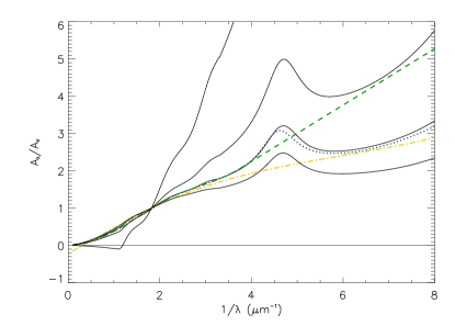
Figure 1: The CCM parameterisation of the Milky Way extinction curve (solid black line) for four different $R_{V}$ (0.5, 2, 3.1 and 4) where the highest values of $R_{V}$ correspond to the flattest curves. We also show the Fitzpatrick parameterisation (dotted blue) with $R_{V}=3.1$, the Prévot law for SMC-like extinction (dashed green) with $R_{V}=3.1$ and the starburst extinction law (dashed dotted yellow) with the preferred value for starburst galaxies $R_{V}=4.05$ (Calzetti et al. 2000). $A_{\lambda}$ is the extinction at wavelength $\lambda$ and $A_{V}$ is the visual extinction.

Since the extinction curves for the Small Magellanic Cloud and starburst galaxies look different compared to the average one for the Milky Way, the extinction curve of the Milky Way may not be representative of high-redshift galaxies. Yet, it is often assumed that the Galactic laws can be applied to dust in other galaxies, e.g. when correcting the light from supernovae for host galaxy extinction. In this paper, such an assumption is relaxed.

3 Fitting dust extinction properties

We have gathered data for a small number of quasars with foreground galaxies, from the literature. We require that the redshift of both the quasar and the galaxy have been determined spectroscopically. We only consider systems for which apparent magnitudes have been measured in at least four different filters, which are in the wavelength range of the redshifted, quasar spectral template. Given these restrictions, our sample of quasar-galaxy systems consists of 21 foreground galaxies with a total of 48 quasar images. Information about these pairs are listed in Table 1.

Table 1: Information about the quasar-galaxy pairs in our sample. $z_{Q}$ is the redshift of the quasar and $z_{G}$ is the redshift of the galaxy. The last two columns list what filters were used in our analysis and the references for the magnitudes.

Quasar	Images	$z_{Q}$	$z_{G}$	Galaxy type	Filters	Source
SDSS J131058.13+010822.2	A	1.39	0.04	star forming	u g r i z	1
Q2237+030	A B C D	1.69	0.04	late	F160W F205W F555W F675W F814W	2
SDSS J114719.89+522923.1	A	1.99	0.05	starburst	u g r i z	1
SDSS J084957.97+510829.0	A	0.58	0.07	starburst	u g r i z	1
SDSS1155+6346	A B	2.89	0.18	early	F160W F555W F814W K	2, 3
MG1654+1346	A	1.74	0.25	elliptical	F160W F555W F675W F814W	2
CXOCY J220132.8-320144	A B	3.90	0.32	spiral	g r i Ks	4
SDSS J0903+5028	A B	3.61	0.39	early	F160W F555W F814W r i	2, 5
SDSS J0924+0219	A B C	1.52	0.39	elliptical	u g r i F160W F555W F814W	2, 6
CLASS B1152+199	A B	1.02	0.44	late	F160W F555W F814W I R V	2, 7
HE0435-1223	A B C D	1.69	0.45	S0	F160W F555W F814W i g r	2, 8
Q0142-100	A B	2.72	0.49	early	F160W F555W F675W F814W	2
HE0230-2130	A1 A2 B C	2.16	0.52	S0/Sa	B R I K F814W F555W	2, 9
BRI0952-0115	A B	4.43	0.63	elliptical	F160W F555W F675W F814W	2
WFI2033-4723	A1 A2 B C	1.66	0.66	Sb/Sc	F160W F555W F814W i	2, 10
SDSS J1004+4112	A B C D	1.74	0.68	cluster of galaxies	u g r i z F160W F555W F814W	2, 11
J1004+1229	A B	2.65	0.95	elliptical	F160W F555W F814W I	2
MG0414+0534	A1 A2 B C	2.64	0.96	early	F160W F110W F205W F675W F814W	2
SDSS J012147.73+002718.7	A	2.22	1.39	unknown	u g r i z	1
SDSS J145907.19+002401.2	A	3.01	1.39	unknown	u g r i z	1
SDSS J144612.98+035154.4	A	1.95	1.51	unknown	u g r i z	1

Most of these are found from strong lensing surveys. However, three of them comes from analysing the quasar spectra (Wang et al. 2004) and an additional three are found from coordinate matching (Östman et al. 2006).

To test whether our sample of 21 quasars with foreground galaxies differs in the colours from the main bulk of quasars, we estimate the rest-frame $B-V$ colour, by K-correcting from the observed bands, for our set of quasars and compare it with a reference set from release three of the Sloan Digital Sky Survey (SDSS) (Schneider et al. 2005). Table 2 contains the estimated values of $B-V$ for our images, and Figure 2 shows the histogram of the two distributions.

Table 2: Estimated rest-frame $B-V$ colour for the different quasar images in our sample.

Quasar	Images	$B-V$
SDSS J131058.13+010822.2	A	0.8
Q2237+030	A B C D	3.4, 2.1, 3.6, 3.4
SDSS J084957.97+510829.0	A	1.1
SDSS1155+6346	A B	1.5, 1.1
MG1654+1346	A	0.4
CXOCY J220132.8-320144	A B	1.7, 1.8
SDSS J0903+5028	A B	0.7, 0.5
SDSS J0924+0219	A B C	0.4, 0.6, 0.2
CLASS B1152+199	A B	1.8, 1.7
HE0435-1223	A B C D	1.1, 1.0, 1.0, 1.0
Q0142-100	A B	0.1, 0.1
HE0230-2130	A1 A2 B C	0.4, 0.2, 0.3, 0.8
BRI0952-0115	A B	0.7, 0.8
WFI2033-4723	A1 A2 B C	0.4, -0.1, -0.3, -0.1
SDSS J1004+4112	A B C D	0.1, 0.6, 0.3, 1.6
J1004+1229	A B	3.9, 5.0
MG0414+0534	A1 A2 B C	2.9, 3.1, 2.8, 2.8
SDSS J012147.73+002718.7	A	1.0
SDSS J145907.19+002401.2	A	0.9
SDSS J144612.98+035154.4	A	0.8

Figure 2: A histogram over rest-frame $B-V$ for the quasars in SDSS DR3 (solid line), and for the quasar images in our sample (dashed line).

We find that our set is redder than the comparison set. The difference in mean rest-frame $B-V$ between the two sets is 0.7 magnitudes. There is also one quasar, WFI2033-4723, for which three out of its four images are significantly bluer than the reference set. The two distributions of rest-frame colours were compared using the Kolmogorov-Smirnov test, yielding a negligible probability that the difference is only due to statistical fluctuations. We conclude that there must be quasars in our sample whose colours are affected by reddening in the intervening galaxy.

The quasar spectral template used, is a combination of the HST radio-quiet composite spectrum (Telfer et al. 2002), and the SDSS median composite spectrum (Vanden Berk et al. 2001). To simulate the effects of dust attenuation, the template spectrum is redshifted and reddened, by different values of $R_{V}$ and $E(B-V)$. This enables synthetic colours to be estimated for dust-reddened quasars. To determine the values of the dust parameters that best describe the observed magnitudes, we compare the observed colours with the synthetic colours for different $R_{V}$ and $E(B-V)$. When choosing colours $X=i-j$ to compare among all possible filter combinations, we want to use the colour combinations that have the greatest potential to separate cases of reddening from those of no reddening. We select the combinations that provide a large difference between observed colour and expected colour without dust extinction, $E(i-j)$, and have small errors. We select colours by maximising the sum over $Q_{ij}$, which is defined by

$$Q_{ij}=\frac{\left[E(i-j)\right]^{2}}{\sigma_{ij}^{2}},$$ (3)

where $\sigma_{ij}$ is the total error of the colour difference, i.e. the errors of the observed magnitudes combined with the uncertainty in the template colours. The sum over $Q_{ij}$ runs over $f-1$ colours where $f$ is the number of filters, and each filter must be used at least once. The colours chosen from maximising the sum over $Q_{ij}$ are used when calculating the $\chi^{2}$ described below. For example, when observations are available in the $ugri$ filter set, the six possible colour combinations are $u-g$, $u-r$, $u-i$, $g-r$, $g-i$ and $r-i$. We assume that $Q_{ug}$ and $Q_{ui}$ have the largest values of $Q_{ij}$. From the remaining four combinations, $u-r$, $g-r$, $g-i$ and $r-i$, we can only choose from $u-r$, $g-r$, and $r-i$, because the colour $u-i$ can be constructed by combining the colours we have already picked, $u-g$ and $u-i$. We then choose the filter combination, of the three remaining, with the largest $Q_{ij}$ to obtain the three colours to be used in the analysis.

For each quasar image, the best-fit dust extinction is determined by comparing the synthetic colours, $X_{\rm syn}=X_{\rm syn}[R_{V},E(B-V)]$, with the observed ones, $X_{\rm obs}$, and minimising the $\chi^{2}=\chi^{2}[R_{V},E(B-V)]$, which is defined to be

$$\chi^{2}=(X_{\rm syn}-X_{\rm obs})^{T}{\cal V}^{-1}(X_{\rm syn}-X_{\rm obs}).$$ (4)

${\cal V}$ is the covariance matrix including the errors from the observed and synthetic colours. The errors of the synthetic colours account for both the intrinsic variability of quasars, and the possible dust extinction in the host galaxy of the quasar. These errors are calculated from a set of quasars with similar redshifts ($|\Delta z|<0.05$), without any resolved foreground galaxies. These were taken from the third data release of the Sloan Digital Sky Survey (Schneider et al. 2005). Their colours were $K$-corrected from the SDSS filters, to the filters used in the observations considered in this work. To avoid a large impact from colour outliers, quasars with a colour differing by more than three standard deviations from the mean were excluded. About 12% of the quasars were rejected by this cut. In Figure 3, the uncertainties for the colours from the template are shown for the SDSS filters at different redshifts.

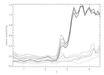
Figure 3: Uncertainties in the template colours for $u-g$, $u-r$, $u-i$, $u-z$, $g-r$, $g-i$, $g-z$, $r-i$, $r-z$, $i-z$ (from black to light grey) as a function of redshift $z$.

As can be seen in the figure, all colours involving the $u$ band have very large errors for quasars with $z\gtrsim 2.5$. It is also at $z\sim 2.5$ that the number of available comparison quasars falls drastically. The covariance matrix also includes the correlations between estimated magnitudes in different filters and consideration to the fact that the same filter can appear more than once in a set of colour comparisons.

The quasar images were fitted with both the CCM law and the Fitzpatrick law with $R_{V}$ and $E(B-V)$ as free parameters. We also considered SMC like extinction, according to the Prévot law. The CCM law that we use is the improved version of the relation by Cardelli et al. (1989), where the extinction law, for the wavelength range 1.1 $\mu$m^-1 $\leq 1/\lambda\leq$ 3.3 $\mu$m^-1, has been exchanged for the curve provided by O’Donnell (1994). The Prévot law used here consists of two parts. For $\lambda<2700$ Å, we use a linear fit to the SMC data in Prévot et al. (1984), and at longer wavelengths we use the extinction law by Fitzpatrick (1999).

In addition to dust in the foreground galaxy, we have also investigated the possibility of extinction in the host galaxy of the quasar.

Table 3: Best fits of $R_{V}$ and $E(B-V)$ together with the 1$\sigma$ uncertainties. Note that the lowest possible value for $R_{V}$ here is 0.1, since $R_{V}=0$ usually is not defined. Also note that for some redshifts and filter combinations, there is no $R_{V}$ dependence for the Prévot law. The interval is then given as $0.1-6.0$. $z_{d}$ is the redshift of the dust extinction, which is $z_{G}$ for foreground extinction and $z_{Q}$ for host extinction. $d$ is the impact parameter expressed in kpc. When this was unavailable, it is marked with a hyphen in the table. When several laws and/or dust redshifts is either fitted for one image, they are all listed in the table below. The probability for each to obtain a higher $\chi^{2}$ value than what was obtained for the fit is given in the last column. We include all fits with a probability larger than 0.5%. The different images are separated by a horizontal line.

Quasar	Image	$z_{d}$	d (kpc)	$R_{V}$	$E(B-V)$	Law	Prob
SDSS J131058.13+010822.2	A	0.04	15.0	3.5 (1.4-6.0)	0.3 (0.2-0.4)	CCM	96 %
SDSS J131058.13+010822.2	A	0.04	15.0	3.5 (1.8-6.0)	0.3 (0.2-0.4)	Fitzpatrick	94 %
SDSS J131058.13+010822.2	A	0.04	15.0	3.5 (1.8-6.0)	0.3 (0.2-0.4)	SMC	95 %
SDSS J131058.13+010822.2	A	1.39	15.0	0.1 (0.1-2.5)	0.1 (0.1-0.2)	Host CCM	12 %
SDSS J131058.13+010822.2	A	1.39	15.0	1.1 (0.3-2.2)	0.1 (0.0-0.2)	Host Fitzpatrick	46 %
SDSS J131058.13+010822.2	A	1.39	15.0	0.1 (0.1-6.0)	0.1 (0.1-0.2)	Host SMC	20 %
Q2237+030	A	0.04	0.7	0.1 (0.1-0.2)	0.7 (0.5-0.9)	Fitzpatrick	1 %
Q2237+030	A	0.04	0.7	0.1 (0.1-0.2)	0.7 (0.5-0.8)	SMC	2 %
Q2237+030	C	0.04	0.6	0.1 (0.1-0.2)	1.2 (0.9-1.4)	CCM	11 %
Q2237+030	C	0.04	0.6	0.2 (0.1-0.6)	0.8 (0.6-1.0)	Fitzpatrick	4 %
Q2237+030	C	0.04	0.6	0.2 (0.1-0.6)	0.8 (0.6-1.0)	SMC	4 %
Q2237+030	D	0.04	0.7	0.3 (0.1-0.6)	0.7 (0.5-0.9)	CCM	56 %
Q2237+030	D	0.04	0.7	0.9 (0.6-1.3)	0.5 (0.3-0.7)	Fitzpatrick	23 %
Q2237+030	D	0.04	0.7	0.9 (0.6-1.3)	0.5 (0.3-0.7)	SMC	23 %
SDSS J114719.89+522923.1	A	0.05	-	0.1 (0.1-3.0)	0.2 (0.1-0.4)	CCM	22 %
SDSS J114719.89+522923.1	A	0.05	-	0.3 (0.1-1.6)	0.2 (0.0-0.3)	Fitzpatrick	65 %
SDSS J114719.89+522923.1	A	0.05	-	1.0 (0.1-5.4)	0.2 (0.1-0.4)	SMC	6 %
SDSS J114719.89+522923.1	A	1.99	-	0.1 (0.1-3.3)	0.0 (0.0-0.1)	Host CCM	5 %
SDSS J114719.89+522923.1	A	1.99	-	0.6 (0.4-2.4)	0.0 (0.0-0.1)	Host Fitzpatrick	18 %
SDSS J114719.89+522923.1	A	1.99	-	2.5 (0.1-6.0)	0.1 (0.0-0.1)	Host SMC	14 %
SDSS J084957.97+510829.0	A	0.07	20.0	2.3 (0.9-3.6)	0.5 (0.4-0.7)	CCM	67 %
SDSS J084957.97+510829.0	A	0.07	20.0	2.2 (1.2-3.2)	0.5 (0.4-0.7)	Fitzpatrick	88 %
SDSS J084957.97+510829.0	A	0.07	20.0	2.2 (0.9-3.5)	0.6 (0.4-0.7)	SMC	62 %
SDSS J084957.97+510829.0	A	0.58	20.0	0.1 (0.1-6.0)	0.3 (0.2-0.4)	Host SMC	2 %
SDSS1155+6346	B	2.89	0.6	6.0 (0.1-6.0)	0.1 (0.0-0.2)	Host CCM	1 %
MG1654+1346	A	0.25	11.3	0.1 (0.1-0.5)	0.2 (0.0-0.3)	SMC	1 %
CXOCY J220132.8-320144	A	0.32	-	2.2 (1.5-3.1)	0.8 (0.7-1.0)	CCM	1 %
CXOCY J220132.8-320144	A	0.32	-	2.4 (1.8-3.3)	0.8 (0.6-1.0)	Fitzpatrick	1 %
CXOCY J220132.8-320144	A	0.32	-	2.5 (1.9-3.5)	0.8 (0.6-1.0)	SMC	1 %
CXOCY J220132.8-320144	A	3.90	-	0.6 (0.1-3.0)	0.1 (0.1-0.2)	Host CCM	3 %
CXOCY J220132.8-320144	A	3.90	-	1.1 (0.2-2.3)	0.1 (0.0-0.2)	Host Fitzpatrick	25 %
CXOCY J220132.8-320144	A	3.90	-	6.0 (0.1-6.0)	0.2 (0.2-0.2)	Host SMC	8 %
CXOCY J220132.8-320144	B	0.32	-	2.2 (1.4-3.2)	0.8 (0.6-0.9)	CCM	1 %
CXOCY J220132.8-320144	B	3.90	-	0.1 (0.1-3.7)	0.1 (0.1-0.3)	Host CCM	8 %
CXOCY J220132.8-320144	B	3.90	-	1.4 (0.4-3.0)	0.1 (0.0-0.2)	Host Fitzpatrick	26 %
CXOCY J220132.8-320144	B	3.90	-	6.0 (0.1-6.0)	0.2 (0.1-0.2)	Host SMC	4 %
SDSS J0903+5028	A	3.61	10.5	2.2 (0.1-3.0)	0.2 (0.1-0.3)	Host CCM	82 %
SDSS J0903+5028	A	3.61	10.5	2.9 (2.5-3.2)	0.3 (0.2-0.3)	Host Fitzpatrick	81 %
SDSS J0903+5028	B	0.39	3.4	2.3 (1.1-4.5)	0.6 (0.4-0.8)	CCM	92 %
SDSS J0903+5028	B	0.39	3.4	2.8 (1.8-4.3)	0.5 (0.3-0.7)	Fitzpatrick	92 %
SDSS J0903+5028	B	0.39	3.4	2.8 (1.8-4.4)	0.5 (0.3-0.7)	SMC	91 %
SDSS J0903+5028	B	3.61	3.4	0.2 (0.1-4.1)	0.1 (0.1-0.4)	Host CCM	45 %
SDSS J0903+5028	B	3.61	3.4	0.6 (0.2-3.4)	0.0 (0.0-0.3)	Host Fitzpatrick	92 %
SDSS J0903+5028	B	3.61	3.4	0.1 (0.1-6.0)	0.1 (0.1-0.2)	Host SMC	96 %
Q0142-100	A	0.49	10.9	6.0 (2.5-6.0)	0.1 (0.0-0.2)	CCM	15 %
Q0142-100	A	0.49	10.9	6.0 (2.7-6.0)	0.1 (0.0-0.2)	Fitzpatrick	15 %
Q0142-100	A	0.49	10.9	6.0 (2.5-6.0)	0.1 (0.0-0.2)	SMC	14 %
Q0142-100	A	2.72	10.9	6.0 (0.1-6.0)	0.1 (0.0-0.2)	Host CCM	61 %
Q0142-100	A	2.72	10.9	6.0 (1.7-6.0)	0.1 (0.0-0.1)	Host Fitzpatrick	48 %
Q0142-100	A	2.72	10.9	0.1 (0.1-6.0)	0.0 (0.0-0.1)	Host SMC	2 %
Q0142-100	B	0.49	2.2	-	0.0 (0.0-0.1)	all	21 %
BRI0952-0115	A	0.63	4.3	0.1 (0.1-3.4)	0.2 (0.1-0.3)	CCM	18 %
BRI0952-0115	A	0.63	4.3	0.5 (0.2-2.0)	0.2 (0.1-0.4)	Fitzpatrick	33 %
BRI0952-0115	A	0.63	4.3	0.1 (0.1-1.6)	0.4 (0.1-0.6)	SMC	35 %
BRI0952-0115	A	4.43	4.3	4.2 (0.1-5.4)	0.1 (0.0-0.4)	Host CCM	26 %
BRI0952-0115	A	4.43	4.3	4.0 (1.0-5.7)	0.1 (0.0-0.3)	Host Fitzpatrick	27 %
BRI0952-0115	A	4.43	4.3	0.1 (0.1-6.0)	0.0 (0.0-0.0)	Host SMC	6 %

Quasar	Image	$z_{d}$	d (kpc)	$R_{V}$	$E(B-V)$	Law	Prob
BRI0952-0115	B	0.63	2.4	0.1 (0.1-3.7)	0.2 (0.1-0.3)	CCM	33 %
BRI0952-0115	B	0.63	2.4	0.5 (0.2-2.1)	0.2 (0.1-0.4)	Fitzpatrick	65 %
BRI0952-0115	B	0.63	2.4	0.1 (0.1-2.7)	0.4 (0.1-0.6)	SMC	42 %
BRI0952-0115	B	4.43	2.4	4.1 (0.1-5.4)	0.1 (0.0-0.4)	Host CCM	53 %
BRI0952-0115	B	4.43	2.4	3.8 (0.9-5.7)	0.1 (0.0-0.3)	Host Fitzpatrick	55 %
BRI0952-0115	B	4.43	2.4	0.1 (0.1-6.0)	0.0 (0.0-0.0)	Host SMC	9 %
MG0414+0534	A1	0.96	9.7	1.5 (1.4-1.6)	1.7 (1.5-1.8)	Fitzpatrick	16 %
MG0414+0534	A1	0.96	9.7	1.3 (1.2-1.5)	1.8 (1.7-2.0)	SMC	58 %
MG0414+0534	A2	0.96	9.5	1.5 (1.5-1.7)	1.9 (1.8-2.1)	Fitzpatrick	3 %
MG0414+0534	A2	0.96	9.5	1.4 (1.3-1.5)	2.1 (1.9-2.3)	SMC	18 %
MG0414+0534	B	0.96	10.5	1.5 (1.3-1.6)	1.6 (1.4-1.7)	Fitzpatrick	19 %
MG0414+0534	B	0.96	10.5	1.2 (1.1-1.5)	1.8 (1.6-1.9)	SMC	57 %
MG0414+0534	C	0.96	7.3	1.4 (1.3-1.5)	1.5 (1.4-1.7)	Fitzpatrick	6 %
MG0414+0534	C	0.96	7.3	1.2 (1.1-1.4)	1.8 (1.6-1.9)	SMC	64 %
SDSS J012147.73+002718.7	A	1.39	-	0.1 (0.1-3.8)	0.1 (0.1-0.2)	CCM	58 %
SDSS J012147.73+002718.7	A	1.39	-	2.0 (1.1-3.2)	0.2 (0.1-0.2)	Fitzpatrick	70 %
SDSS J145907.19+002401.2	A	1.39	-	0.1 (0.1-3.8)	0.1 (0.1-0.2)	CCM	3 %
SDSS J145907.19+002401.2	A	1.39	-	2.2 (0.2-5.9)	0.2 (0.0-0.4)	Fitzpatrick	5 %
SDSS J145907.19+002401.2	A	1.39	-	0.1 (0.1-6.0)	0.2 (0.1-0.2)	SMC	2 %
SDSS J145907.19+002401.2	A	3.01	-	0.3 (0.3-0.8)	0.0 (0.0-0.0)	Host Fitzpatrick	5 %
SDSS J145907.19+002401.2	A	3.01	-	3.0 (0.1-6.0)	0.1 (0.1-0.1)	Host SMC	12 %

4 Results and discussion

Of the 48 images, 26 yielded inconclusive results. The chi-square of their fits was so high that, if they had been affected by dust following our extinction laws, there was only a 0.5% probability that such a high chi-square value would be obtained. However, a poor fit does not automatically imply that there is a strange, unknown reddening law. It can also be the result of for example (1) underestimated observational errors, (2) the extinction law having more degrees of freedom than the laws we have assumed, (3) peculiar quasars that have an intrinsic spectrum that differs significantly from the template, (4) effects from other intervening objects that are unresolved in the available images, (5) microlensing effects, or (6) changes in colour due to the time variability of the quasar. The significance of the latter two possibilities, when comparing quasar images, are discussed in Yonehara et al. (2007).

The fit results for the remaining 22 images (corresponding to 13 galaxies) are presented in Table 3. In Figure 4, a few of the confidence levels obtained from the $\chi^{2}$ fitting of the quasar images are shown.

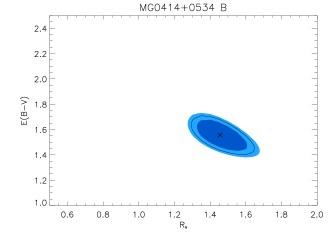
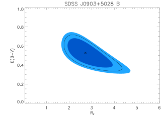
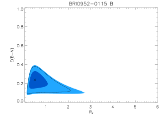
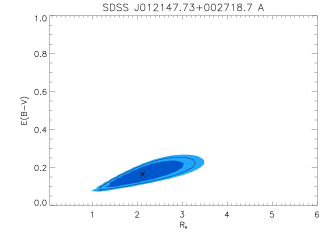
Figure 4: Confidence levels for some of the quasar images that could be fitted by dust extinction in the intervening galaxy using the Fitzpatrick extinction law. The levels correspond to 1$\sigma$ for one parameter (black line) and 68% (dark blue region) and 90% (pale blue) for two parameters.

The error intervals in Table 3 indicate the $1\sigma$ uncertainty. The errors are calculated with the assumption that the extinction law is valid for a positive colour excess, and for all positive values of $R_{V}$ up to 6.0. Negative values of $E(B-V)$ are not expected for normal quasars, affected by dust. However, an intrinsically blue quasar is best fitted with a negative $E(B-V)$. For small and negative values of $R_{V}$ ($\lesssim 0.7$), the extinction laws have a peculiar behaviour (see e.g. the CCM parameterisation with $R_{V}=0.5$ in Figure 1). The non-smooth function, and the negative values of the extinction $A_{\lambda}/A_{V}$, are probably hard to explain using a physical dust model. We chose however to consider all fits, down to $R_{V}=0$. For large (positive) values of $R_{V}$, the extinction becomes less wavelength-dependent, and it becomes more difficult to distinguish from the case of no extinction. When the colours of a quasar image in our analysis can be explained without dust, there is no limitation on $R_{V}$, because there is no $R_{V}$ dependence in the extinction laws for $E(B-V)=0$.

The law which we refer to as the Prévot law, consists of two parts. For $\lambda<2700$ Å, we use a linear fit to the SMC data in Prévot et al. (1984), and for $\lambda>2700$ Å, we use the parameterisation of the Milky Way extinction by Fitzpatrick (1999). If the foreground galaxy, where the extinction occurs, is located at low redshift, most of the filters used for observations will correspond to regions of the spectrum that are affected by the second part of the extinction curve, which is identical to the Fitzpatrick law ($\lambda>2700$ Å). If, on the other hand, the extinction redshift is high, the filters will correspond to regions of the spectrum that are affected by the first part of the extinction curve. This part has the relation $A_{\lambda}/E(B-V)=a+bx+R_{V}$. It is therefore not possible to estimate $R_{V}$ from the observed colour, e.g. $B-V$, because the $R_{V}$ dependence is subtracted out, $B-V=A_{B}-A_{V}=E(B-V)(a+bx_{B}+R_{V})-E(B-V)(a+bx_{V}+R_{V})=E(B-V)(bx_{B}-bx_{V})$. This is not the case for e.g. the Fitzpatrick or CCM law. For objects which have high extinction redshifts, no preferred value of $R_{V}$ can be determined for SMC-like extinction, using this parameterisation. The same problem occurs for the CAB law, where a preferred value of $R_{V}$ cannot be determined for any extinction redshift, because the extinction law provides colours that are independent of $R_{V}$. This is because the parameterisation we use is $A_{\lambda}/E(B-V)=a+bx+cx^{2}+dx^{3}+R_{V}$, and thus $B-V=A_{B}-A_{V}$ is not dependent on $R_{V}$. This should be remembered when studying the fitted values in Table 3.

We note that even though we have considered both intervening and host extinction, only host extinction cannot explain the difference in $B-V$ that we see, when comparing the colours of our quasars with quasars without intervening galaxies (see Figure 2). Furthermore, we have taken the possibility of dust extinction within the host into account, in the calculation of the covariance matrix.

In Figure 5, observed colours are plotted together with the best synthetic dust colours for each of the quasar images, that could be fitted by dust (i.e. the images in Table 3). In the figure, comparison is made with the synthetic magnitude at the longest wavelength arbitrarily adjusted to match the observations. However, this was not the case in the actual fitting procedure, which involves only differences in magnitudes.

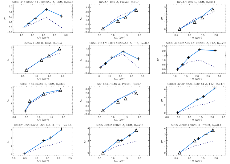
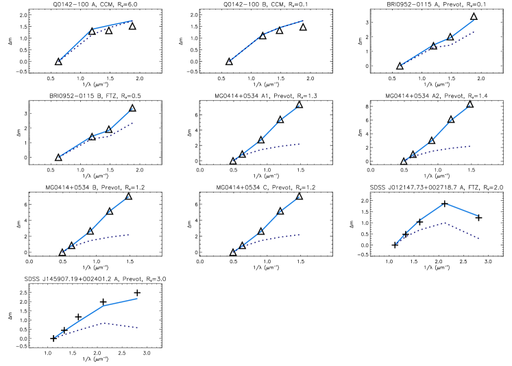
Figure 5: Comparison of the measured magnitudes (black signs) with the fitted magnitudes (light blue solid line) for the images that could be fitted using the dust laws. The dark blue dotted line shows the expected magnitudes without dust. Note that sometimes only one line is visible when the best fit is with little or no extinction. The ground-based measurements are marked with plus signs while the HST observations are marked with triangles. All magnitudes are normalised so that the magnitude at the longest wavelength is zero.

In all of these cases, the fitted magnitudes agree very well with observed values.

4.1 The badly fitted quasar images

In Figure 6, we show how well the best extinction law agrees with observed magnitudes for each of the quasar images that could not be fitted with regular dust extinction.

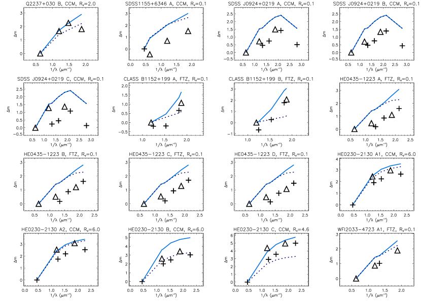
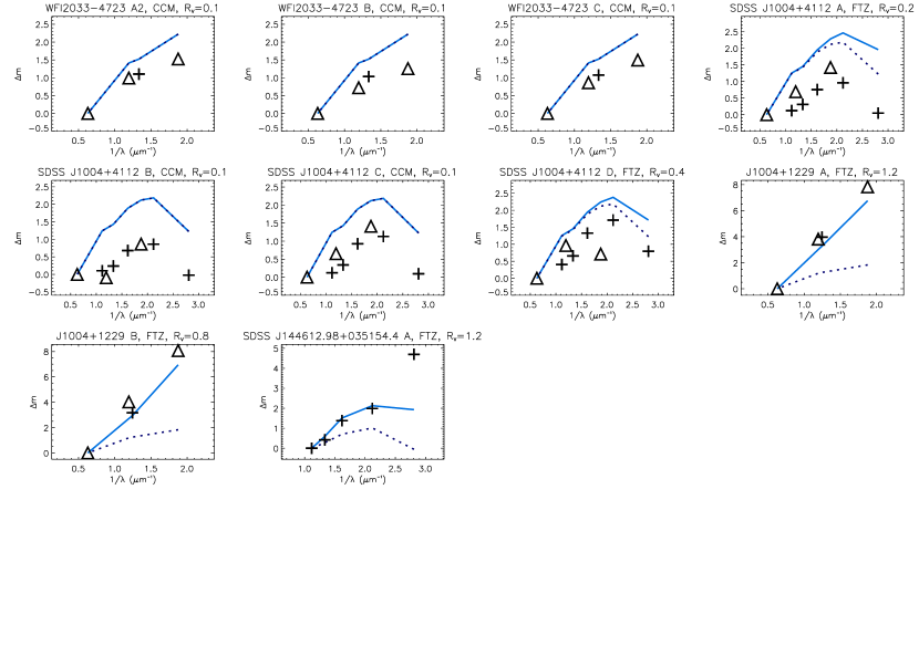
Figure 6: Comparison of the measured magnitudes (black signs) with the fitted magnitudes (light blue solid line) for the images that were badly fitted using the dust laws. The dark blue dotted line shows the expected magnitudes for no extinction. Note that sometimes only one line is visible when the best fit is with little or no extinction. The ground-based measurements are marked with plus signs while the HST observations are marked with triangles. All magnitudes are normalised so that the magnitude at the longest wavelength is zero.

A possible explanation for the difficulty in fitting some of the quasar images with the reddened template is that in some cases, observations of the same image in different filters were made at different times. If the object is variable, and has changed significantly between the times of observations for the different filter sets (e.g. HST and ground-based), this could lead to erroneous observed colours, which cannot be correctly fitted by dust. One possible example is SDSS J1004+4112 where the ground-based and HST observations appear to be shifted with respect to each other (see Figure 6). Therefore, in the cases where we have enough data points, we separate the HST and ground-based observations to see if this will provide a good fit. There are 11 quasar images that have observations in a minimum of four different filters, which are either ground-based or space-based. When applying our analysis to these data, we find that two of the images of HE0230-2130 can be described by dust extinction. The best-fit values are provided in Table 4.

Table 4: Additional best fits of $R_{V}$ and $E(B-V)$ together with the 1$\sigma$ uncertainties for quasar images which are likely to be dust extincted. The first three quasar images are badly described when using both HST and ground-based images, but are possible to fit with dust when using only the ground-based measurements. The last image is one where the $u$ band magnitude seems to be deviant from the other magnitudes and we have made a fit without it.

Quasar	Image	$z_{d}$	d (kpc)	$R_{V}$	$E(B-V)$	Law	Prob	Comment
HE0230-2130	A2	0.52	6.1	3.2 (1.5-5.4)	0.2 (0.1-0.2)	CCM	13 %	ground
HE0230-2130	A2	0.52	6.1	3.4 (1.8-6.0)	0.2 (0.1-0.2)	Fitzpatrick	12 %	ground
HE0230-2130	A2	0.52	6.1	4.0 (1.6-6.0)	0.2 (0.1-0.3)	SMC	15 %	ground
HE0230-2130	A2	2.16	6.1	0.1 (0.1-3.0)	0.1 (0.1-0.1)	Host CCM	1 %	ground
HE0230-2130	A2	2.16	6.1	1.7 (0.4-2.8)	0.1 (0.0-0.1)	Host Fitzpatrick	4 %	ground
HE0230-2130	A2	2.16	6.1	6.0 (0.1-6.0)	0.1 (0.1-0.1)	Host SMC	4 %	ground
HE0230-2130	B	0.52	8.0	2.6 (0.5-4.2)	0.3 (0.2-0.3)	CCM	1 %	ground
HE0230-2130	B	0.52	8.0	2.9 (0.7-5.7)	0.3 (0.1-0.3)	Fitzpatrick	1 %	ground
HE0230-2130	B	0.52	8.0	3.7 (1.4-6.0)	0.3 (0.2-0.3)	SMC	1 %	ground
HE0230-2130	B	2.16	8.0	6.0 (0.1-6.0)	0.1 (0.1-0.1)	Host SMC	1 %	ground
SDSS J144612.98+035154.4	A	1.51	-	2.0 (0.1-2.0)	0.2 (0.1-0.3)	CCM	26 %	no u
SDSS J144612.98+035154.4	A	1.51	-	2.0 (1.4-2.0)	0.2 (0.1-0.2)	Fitzpatrick	32 %	no u
SDSS J144612.98+035154.4	A	1.95	-	1.1 (0.9-1.5)	0.1 (0.1-0.1)	Host Fitzpatrick	9 %	no u

When calculating the errors of the synthetic colours, we defined colour outliers as quasars with a colour differing by more than three standard deviations from the mean. This led to the exclusion of 12% of the quasars in our reference set. Thus we would expect about 2.5 of our 21 quasars to be colour outliers, if our sample is as homogeneous as the SDSS sample. Some of the badly-fitted quasar data could correspond to so-called peculiar quasars, differing significantly from the template in one or several filters.

If a deviation is observed in only one filter, it could be explained by a strong absorption or emission feature, which is redshifted into the wavelength region of the filter of observation. Some badly-fitted images, such as SDSS J144612.98+035154.4, have colours that agree well with synthetic dust colours, apart from one band (see Figure 6). For these, we make the assumption that the diverging magnitude is erroneous and redo the fit without. Because observations in at least four filters are required, there is only one case of interest, SDSS J144612.98+035154.4. The best-fit values for this system, when removing the $u$ band magnitude are provided in Table 4.

4.2 Global results

To understand how the fitted values of $R_{V}$ are distributed, we assume that all quasars are affected by dust extinction in the intervening galaxy, following the Fitzpatrick law. For each image, we calculate a probability distribution for $R_{V}$, by locating the maximum $\chi^{2}$ probability for each $R_{V}$, when $E(B-V)$ is set free. The maximum of the distribution will have the same value, as the probability for the Fitzpatrick law, in Table 3. The probability distributions for all images that could be fitted with dust, are then added together. In this way, we take into account the possibility of non-Gaussian distributions, and the result is weighted by the probability of the fit. We exclude images for which our fits are consistent with almost no extinction because the $R_{V}$ dependence is weak then. The result is presented in Figure 7, where it is evident that the inclusion of the objects in Table 4, does not affect the shape of the curve significantly.

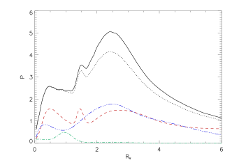
Figure 7: The co-added probability distributions for the fits with intervening dust following the Fitzpatrick extinction law, weighted by the probability of the fit. The dotted line shows the added probability when using the well fitted quasar images in Table 3 and the solid line when also the objects in Table 4 are included. The added probabilities for the subset of early-type galaxies (dashed line), late-type galaxies (dash-dot) and starburst/star-forming galaxies (dash-dot-dot-dot) are also included in the figure.

Using the larger set, we found a most probable value of $R_{V}$ of 2.4, with a FWHM of 2.7. This value is slightly lower than the Galactic value of 3.1, but well within the range due to the large spread of fitted values. In Figure 8, the best-fit values of $R_{V}$ are plotted as a function of redshift and $E(B-V)$.

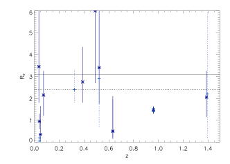
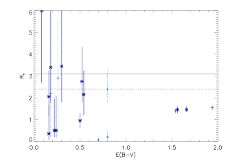
Figure 8: The fitted values of $R_{V}$ with the 1$\sigma$ errorbars for all images that could be fitted using the Fitzpatrick parameterisation of dust in an intervening galaxy. The first panel shows $R_{V}$ as a function of dust redshift and the second as a function of colour excess. In the first panel, the results from the different images of the same quasar will be plotted on top of each other since they all have the same redshift. In the second panel, the results of different images will be plotted in different places along the x axis since $E(B-V)$ differs at least slightly between the images. The fitted values which have a larger probability than 10% (see Table 3) are plotted with stars and dark blue solid errorbars while the less reliable ones, with a smaller probability than 10%, are plotted with plus signs and dotted light blue errorbars. The most probable value of $R_{V}$ found when co-adding the probability distributions for the fits (see Figure 7) is indicated with a dotted line at $R_{V}=$ 2.4.

There are no clear trends in the dependence with these parameters on $R_{V}$.

To test the possibility of a dependence of galaxy type for $R_{V}$, we divide Figure 7 into three plots, one for early-type galaxies, one for late-type galaxies, and one for starburst/star-forming galaxies. These are shown in Figure 7. The plot for the late-type galaxies have less features than the one for all galaxies, but the most probable $R_{V}$ remains similar. The plots for the early-type galaxies and the starburst galaxies are more different. However, these are constructed using only four and three images, respectively. It would be interesting to repeat the same study for a larger number of galaxies in the future.

We note that since a large part of the galaxies studied are lensing galaxies, the sample will not necessarily be representative of the universal galaxy population, because strong-lensing surveys are more efficient in finding massive galaxies.

4.3 Specific systems

Several of the quasar-galaxy systems that we study, have multiple images. Because the multiple images have the same intrinsic colours, the difference in colour between the images should be explained by dust extinction, or possibly by microlensing or time-variability effects. In this section, we compare fits for different images of the same quasar. We also compare with other dust property estimates of the same object from the literature. In Östman et al. (2006), some of the objects here were investigated with a similar method, that has now been improved. The most important improvement is that, while in Östman et al. (2006), we compared all magnitudes with the value in the $u$ band in the expression for the $\chi^{2}$, we here optimise the choice of colours to maximise the probability of detecting a potential dust extinction (see Section 3). Another improvement is that we include the observational errors, in addition to the template errors, in the covariance matrix. Some of the systems that we have studied have also been investigated using the differential method by other authors (Falco et al. 1999; Elíasdóttir et al. 2006; Toft et al. 2000). When we state their preferred values of $R_{V}$ in the text below followed by an interval within parenthesis, this is the error interval of $R_{V}$ provided in that paper.

SDSS J131058.13+010822.2

This quasar-galaxy system was found in Östman et al. (2006), by matching the coordinates of quasars with those of galaxies. The colours of the quasar indicate that it is most likely affected by dust extinction. In that paper, it was found to have $R_{V}=3.4(1.7-5.7)$ using the CCM parameterisation, and $R_{V}=3.4(2.4-4.7)$ using the Fitzpatrick parameterisation. This agrees well with what was found in this analysis, where the preferred value of $R_{V}$ was 3.5.

According to the New York University Value-Added Galaxy Catalog (Blanton et al. 2005), the foreground galaxy is a star-forming galaxy at $z=0.04$. Fitting the quasar colours with starburst-like extinction according to the CAB law, we find a best fit $E(B-V)$ of 0.3 (0.2-0.4), where the $\chi^{2}$ provides a probability of 99%.

Q2237+030

There are four images of this quasar, three of them can be fitted with dust extinction in the intervening galaxy, all with unrealistically low values of $R_{V}$ and an $E(B-V)$ between 0.5 and 1.2, depending upon which image is studied and the parameterisation that is used. The extremely low preferred values of $R_{V}$ for image A and C, are difficult to justify physically due to the strange appearance of the extinction laws for low $R_{V}$ (e.g. see the CCM parameterisation with $R_{V}=0.5$ in Figure 1). Image D has a larger $R_{V}$ value, with a higher chi-square probability. Image B, which has one deviating band, could not be fitted by dust extinction.

The extinction properties of this system have been measured by Falco et al. (1999), using the differential method. They obtained a high value of $R_{V}$ of $5.29(4.47-6.11)$, which is inconsistent with our result. Elíasdóttir et al. (2006) used the same technique and derived values of $R_{V}$ between 2.9 and 3.1, with errors of the order of 1.5. In our analysis, values below 1.3, were obtained.

We note that the colours of the object have been shown to vary with time (Moreau et al. 2005) and therefore there must be an effect, in addition to or instead of dust extinction, affecting the colours, for example microlensing. This would explain why we derive best-fit values for $R_{V}$ that are unrealistically low, and why completely different values have been obtained using other data sets.

SDSS J114719.89+522923.1

This case of a quasar shining through a galaxy, was discovered by Östman et al. (2006). However, no $R_{V}$ could be determined. König et al. (2006) have since detected absorption features from the intervening galaxy in the quasar spectrum strengthening the assumption that the colours of this quasar are affected by dust absorption in the intervening galaxy. In this paper, we found that the colours are best-fitted by dust in the intervening galaxy, with a low $R_{V}$.

According to the New York University Value-Added Galaxy Catalog (Blanton et al. 2005), the foreground galaxy is a starburst galaxy at $z=0.05$. We find that Galactic-like dust describes the observed colours better than typical dust in starburst galaxies. Using the CAB law for starburst extinction, we find a best-fit value of $E(B-V)$ of 0.2, with a $\chi^{2}$ probability of 12%.

SDSS J084957.97+510829.0

This quasar with a foreground galaxy was discovered by Östman et al. (2006). It was found to have a measured value of $R_{V}$ of $1.7(0.7-2.9)$ using the CCM parameterisation, and of $2.2(1.5-2.9)$ using the Fitzpatrick parameterisation. This agrees well with our preferred values of $R_{V}$ for this system, of approximately 2.2-2.3.

According to the New York University Value-Added Galaxy Catalog (Blanton et al. 2005), the foreground galaxy is a starburst galaxy at $z=0.07$. We found that the observed colours of the quasar were reproduced more effectively using the Fitzpatrick extinction curve, than using an extinction curve that should be valid for starburst galaxies. However, the fit with starburst-like extinction according to the CAB law was also good. The best fit with $E(B-V)=0.5$ provided a $\chi^{2}$ probability of 44%.

SDSS1155+6346

This quasar has two images. For one image, we were unable to explain the measured colours by dust extinction, and for the other image, there is only a small probability that the best-fit dust scenario is the true explanation of the colours. The magnitudes of image B could be fairly well-described by dust, if the observational errors were larger. Image A, on the other hand, has a deviating K band magnitude. This is one case where one could suspect problems with the ground-based observations. It would be interesting to observe this object further to investigate if the deviation is a result of the observations, or if it is an interesting feature in the spectrum.

MG1654+1346

The colours of MG1654+1346 could be explained by SMC-like dust in the intervening galaxy, with a low $R_{V}$. However, the $\chi^{2}$ of the fit is high.

CXOCY J220132.8-320144

There are two images of CXOCY J220132.8-320144, both of which could be explained by dust, in particular at the host galaxy with low values of $R_{V}$.

SDSS J0903+5028

This object was studied by Östman et al. (2006), using a different data set. The CCM parameterisation gave $R_{V}=0(0-0.7)$, and the Fitzpatrick parameterisation $R_{V}=0.9(0.7-1.2)$, for the image we will refer to as image A. However, we did not manage to fit this image with intervening extinction here, and we have therefore no $R_{V}$ with which to compare. Instead we found that it could be described by extinction in the host galaxy with an $R_{V}$ of approximately 2.3-2.8. Image B, however, can be reproduced by assuming that there is dust either in the intervening galaxy or in the host galaxy.

SDSS J0924+0219

There are three images of SDSS J0924+0219. The colours within these images cannot be fitted by the extinction laws used in our analysis.

CLASS B1152+199

Using the differential method, both Toft et al. (2000) and Elíasdóttir et al. (2006) have measured $R_{V}$. They obtained $R_{V}=1.3-2.1$ and $R_{V}=2.1(2.0-2.2)$, respectively. In our analysis, we have not managed to find a good fit to the observed magnitudes for any of the two images.

HE0435-1223

There are four images of this quasar. None of these images have measured colours that could be fitted using our extinction laws.

Q0142-100

Using the differential method, Falco et al. (1999) and Elíasdóttir et al. (2006) have measured $R_{V}$ for this system. They obtained $3.11(2.11-4.11)$ and $R_{V}=4.7(4.0-5.4)$, respectively. We find that there is little extinction in this system, causing unreliable $R_{V}$ determinations.

HE0230-2130

None of the four images of HE0230-2130 could be reproduced by taking into account the effects of dust, using both the HST, and the ground-based observations. However, if we use only the ground-based observations, some of the images can be explained by dust, in particular image A2. This is one of few images for which we measure a higher $R_{V}$, than for the Milky Way, 3.2 for the CCM parameterisation and 3.4 for the Fitzpatrick parameterisation.

BRI0952-0115

Falco et al. (1999) fitted a value of $3.10(2.10-4.10)$ for $R_{V}$, using the differential method. With intervening extinction, we found lower values of $R_{V}$.

WFI2033-4723

There are four images of this quasar. None of these images have colours that could be reproduced well by our extinction laws.

SDSS J1004+4112

There are four images of this quasar. The observations could not be fit by assuming dust extinction for any of the images. The ground-based observations appear to follow a smooth curve, but the HST observations appear to be more scattered. However, using only the ground-based observations, we were unable to obtain a good fit, using the extinction laws used in this paper.

J1004+1229

There are two images of this quasar. We were unable to reproduce the colours of either image, using our dust extinction laws.

MG0414+0534

This is an interesting case of a quasar that is heavily reddened. There have been claims both that the reddening is caused by dust in the lens galaxy, and in the host galaxy. Lawrence et al. (1995) reason that the most likely cause is dust extinction in the lens galaxy. They argue that (1) the observed spectrum can be well-explained by dust at intervening redshifts, while extinction in the host galaxy is unable to reproduce the spectrum for Galactic extinction and barely for SMC-like extinction; (2) the separation between the light paths for the different images at the host is too small to explain the difference in colours between the images; in contrast, a separation at the lensing galaxy would be able to reproduce the colour difference better; and (3) two of the reddest quasars that are known, MG 0414+0534 and MG 1131+0456, both have an intervening galaxy, and it is unlikely that both have a foreground galaxy, and that the foreground galaxy is not responsible for the extremely red colours. However, for the case of MG 1131+0456, Kochanek et al. (2000) concluded that dust is not responsible for the red colour, at either redshift. They proposed instead that stellar emission from the host galaxy, could explain the red colours. Tonry & Kochanek (1999) suggest that the red colours of MG0414+0534 are caused by dust extinction in the host. Their arguments are that (1) the visible arc of the host galaxy is bluer than the quasar images and that the extinction must be uniform over a large region, because there is little difference in extinction between quasar images, and no notable difference in colour along the arc; and (2) that the colour and surface brightness of the lens galaxy agrees well with that of a passively-evolving early-type galaxy on the Fundamental Plane (Keeton et al. 1998).

When fitting for dust extinction, we found that the colours of the quasar could be explained by presence of dust in the lens galaxy, but not by dust in the host galaxy alone. All images gave reasonably similar values of $R_{V}$, indicating that the foreground galaxy has a homogeneous dust content. Since there are strong claims of dust extinction in the host galaxy, we decided to measure the likelihood of dust extinction in both galaxies. We fitted for dust extinction at both redshifts with one $R_{V}$ for each redshift, a value of $E(B-V)$ for the host extinction, and a $E(B-V)$ value for each line of sight through the foreground galaxy. We found that the best fit was given by no extinction in the host galaxy [$E(B-V)=0$], and severe extinction in the foreground galaxy [$R_{V}=1.5$, and $E(B-V)=1.6,1.9,1.5,1.5$ for the different sight lines through the galaxy]. Marginalising over $E(B-V)$ for the host galaxy, we find that the $\chi^{2}$ is almost as good for small extinctions $E(B-V)<0.3$ as for the best fit which had $E(B-V)=0$. For higher values of $E(B-V)$, however, the $\chi^{2}$ is much worse (see the first panel of Figure 9). From our analysis, it appears that the bulk of the extinction occurs in the intervening galaxy, but we cannot exclude an additional small extinction in the host.

Figure 9: The $\chi^{2}$ values for different $E(B-V)$ in the host galaxy (first panel) and $R_{V}$ in the intervening galaxy (second panel) for MG0414+0534 .

The best fit for the intervening galaxy is $R_{V}\sim 1.5$, regardless of whether we include extinction in the host or not. In the second panel of Figure 9, there is a marginalisation over $R_{V}$ in the intervening galaxy, showing how the $\chi^{2}$ changes for different $R_{V}$. Falco et al. (1999) found a similar value of $R_{V}$, $1.47(1.32-1.62)$. Elíasdóttir et al. (2006) found values ranging between 0.4 and 3.8, depending on the images that they compared.

SDSS J012147.73+002718.7

The best-fit values for $R_{V}$ from Östman et al. (2006) for this quasar system (3.3 for the CCM parameterisation and 1.8 for the Fitzpatrick parameterisation), are within the 1$\sigma$ uncertainty of our fit.

SDSS J145907.19+002401.2

This object was also studied by Östman et al. (2006). In that paper, the CCM parameterisation provided an $R_{V}$ value of $0(0-0.7)$, and the Fitzpatrick parameterisation, an $R_{V}$ value of $1.8(0.4-3.5)$. These results are consistent with the values derived in this paper.

SDSS J144612.98+035154.4

In Östman et al. (2006), the CCM parameterisation gave $R_{V}=0(0-0.7)$ and the Fitzpatrick parameterisation $R_{V}=1.3(1.0-1.6)$. In this paper, we found no dust model that could explain the colours in a satisfactory way. However, if we ignore the $u$ band magnitude, the colours could be fitted by intervening dust with an $R_{V}$ of 2.0.

5 Summary and conclusions

The reddening of quasars by foreground galaxies has been investigated. At our disposal, we have had 21 quasar-galaxy systems with a total of 48 quasar images. By looking at the rest-frame $B-V$, we conclude that the foreground galaxy, close to the line of sight, must affect the quasar colours. Using redshifted reddened quasar templates, we fit for $R_{V}$ and $E(B-V)$ using the measured colours.

Of the data that we consider, 22 images could be fitted by dust extinction. Assuming dust extinction in the intervening galaxy following the Fitzpatrick law, we find a most probable $R_{V}$ value of 2.4. This value is lower than the Galactic mean value of 3.1. However, the FWHM of our distribution of $R_{V}$ was determined to be 2.7 and thus the Galactic mean value is within the range of the spread. We note that our sample will not be representative of the universal galaxy population because the majority of our quasars were observed by strong lensing surveys, which are particularly efficient in finding massive galaxies. The large spread in values indicates that the dust content can vary significantly between different galaxies. However, we found no strong correlation between the values of $R_{V}$ and redshift, colour excess or galaxy type. In the future, when a larger dataset with superior quality is available, a similar analysis could be of considerable benefit to, for example, the use of extinction-corrected supernovae as distance indicators. It would not be surprising if a correlation was found, because metallicity and elemental abundance ratios are expected to affect dust properties, and both quantities evolve with redshift and galaxy type. Furthermore, there are at least two major mechanisms that create dust grains, the first is in AGB stars (e.g. Mathis 1990) and the second in core-collapse supernovae (e.g. Bank & Clayton 2003), which could give rise to different types of dust.

The uncertainties in the determination of the amount of dust are large, when taking into account the different possible dust models. This fact may be of importance for flux anomalies, used as a probe of cold dark matter substructure (Kochanek & Dalal 2004).

Another interesting observation is that when several images of the same quasar could be fitted by dust, the preferred values of $R_{V}$ were similar. This could indicate that $R_{V}$ has little spread within individual galaxies, but that it varies between galaxies. A caveat, however, is that for many of our quasars one or several of the images could not be fitted by the standard reddening laws we tried, potentially challenging the conclusion of homogeneous dust properties within individual lensing galaxies, unless the colour outliers can be attributed to something different from dust. In total, there were seven quasars in our sample that had several images, one or several of which could be fitted with dust. Three of those quasars had similar values of $R_{V}$, for all images, regardless of extinction law, two quasars had at least one image that could not be reproduced by assuming the presence of dust, one quasar had images where the $R_{V}$ values did not agree with each other, and one quasar was consistent with experiencing no dust extinction.

Several systems were found with low values of $R_{V}$, comparable to what has been measured from global fits, using Type Ia supernova data. However, the distribution of $R_{V}$ for our fits suggests that a large fraction of the galaxies considered in this study are compatible with Milky Way dust. Due to the limited number of objects in our study, as well as the possibility of selection effects and analysis bias, no strong conclusion can be drawn as to whether the extinction properties in foreground galaxies, along the line of sight to quasars, differ or not from extinction in host galaxies of Type Ia supernovae.