Sources of SEP Acceleration during a Flare–CME Event

Abstract

A high-speed halo-type coronal mass ejection (CME), associated with a GOES M4.6 soft X-ray flare in NOAA AR 0180 at S12W29 and an EIT wave and dimming, occurred on 9 November 2002. A complex radio event was observed during the same period. It included narrow-band fluctuations and frequency-drifting features in the metric wavelength range, type III burst groups at metric–hectometric wavelengths, and an interplanetary type II radio burst, which was visible in the dynamic radio spectrum below 14 MHz. To study the association of the recorded solar energetic particle (SEP) populations with the propagating CME and flaring, we perform a multi-wavelength analysis using radio spectral and imaging observations combined with white-light, EUV, hard X-ray, and magnetogram data. Velocity dispersion analysis of the particle distributions (SOHO and Wind in situ observations) provides estimates for the release times of electrons and protons. Our analysis indicates that proton acceleration was delayed compared to the electrons. The dynamics of the interplanetary type II burst identify the burst source as a bow shock created by the fast CME. The type III burst groups, with start times close to the estimated electron release times, trace electron beams travelling along open field lines into the interplanetary space. The type III bursts seem to encounter a steep density gradient as they overtake the type II shock front, resulting in an abrupt change in the frequency drift rate of the type III burst emission. Our study presents evidence in support of a scenario in which electrons are accelerated low in the corona behind the CME shock front, while protons are accelerated later, possibly at the CME bow shock high in the corona.

1 Introduction

Coronal mass ejections (CMEs) are large-scale structures carrying plasma and magnetic field from the Sun. CMEs are associated with flares, filament eruptions, shocks, radio bursts, solar energetic particle (SEP) events, and have been found to be the primary cause of major geomagnetic disturbances and changes in the solar wind flow (see, e.g., Schwenn et al., 2005; Vilmer et al., 2003; Mann et al., 2003; Gopalswamy et al., 2002; Leblanc et al., 2001; Gosling, 1997).

Radio type III bursts are fast frequency-drifting features that can be used as tracers of energetic electrons as they are caused by subrelativistic ($\approx$2.5 to $\approx$80 keV) electron streams travelling outward from the Sun at speeds of about 0.1 c to 0.5 c (see, e.g., Wild, 1950; Dulk, 1985). Near-relativistic electrons (30 – 315 keV) can be observed in situ during SEP events, in association with type III bursts that continue into the IP space (Simnett 2005). Radio type II bursts, on the other hand, are thought to be caused by MHD shock waves propagating through the corona and interplanetary medium (e.g., Nelson and Melrose, 1985). Some studies suggest that coronal metric type II bursts and interplanetary (IP) decameter–hectometer (DH) type II bursts do not have the same driver (e.g., Cane and Erickson, 2005), and that the latter are exclusively created by the CME bow shocks (e.g., Cliver, Webb, and Howard, 1999).

SEPs are believed to be accelerated in the lift-off phase of CMEs, which could include either acceleration in flaring processes (e.g., de Jager, 1986), acceleration in coronal/interplanetary shocks (e.g., Reames, 1999 and references therein), or in both (e.g., Klein and Trottet, 2001; Klein et al., 1999; Kocharov and Torsti, 2002). Recently, the role of CME interaction in SEP production has also been discussed (e.g., Gopalswamy et al., 2002; Kahler, 2003; Wang et al., 2005, and references therein). One of the difficulties in determining the relevant processes lies in the uncertainties of timing. SEPs are typically released no earlier than the maxima of the flare impulsive phases (Kahler, 1994), yet at the time of SEP release the height of the associated CME can vary from one to over ten solar radii (Kahler, 1994; Krucker and Lin, 2000; Huttunen-Heikinmaa, Valtonen, and Laitinen, 2005). It has also been observed that different particle species can be released non-simultaneously (Huttunen-Heikinmaa, Valtonen, and Laitinen, 2005; Krucker and Lin, 2000; Mewaldt et al., 2003).

The in-situ observations of SEPs are strongly influenced by the magnetic connection between the spacecraft and the flare site (e.g., Cane, Reames, and von Rosenvinge, 1988). For example, the nominally well-connected area for the spacecraft in the L1-point is around 60^∘ West on the solar hemisphere. kallenrode93 found that at larger angular distances between the observer’s magnetic footpoint and the flare location, the onsets of energetic particles in relation to the microwave maximum are more delayed, and the proton onsets are relatively more delayed than the electron onsets. Assuming that SEPs originated from the flaring processes, kallenrode93 concluded that the propagation of $\approx$20 MeV protons from the flare site to the connecting magnetic field line is systematically slower than of $\approx$0.5 MeV electrons, and the electron-to-proton ratio tends to increase with angular distance from the flare site. Of course, the modern view of particle acceleration in the solar corona does not rely on flares as the only source of energetic particles during SEP events. Thus, instead of reflecting the azimuthal particle propagation conditions in the corona, the findings of Kallenrode can be re-interpreted as reflecting the azimuthal and/or temporal evolution of the source, usually a coronal shock wave driven/launched by a CME; a delay between the plasma eruption and the observed onset of the SEP event reflects the establishment of the magnetic connection between the source and the observer and/or the efficiency of the acceleration and escape of particles in different parts (bow/flanks) of the global coronal shock wave.

Consistent with the current views and the conclusions of kallenrode93 are the results of krucker99, who found that in some events the injection time of the electrons is consistent with the timing of the type III radio emission, while in other cases the electrons were apparently released up to half an hour later than the start of the type III burst. The non-delayed electron events were concentrated in the well-connected area, while the delayed events were more spread out. Similar delays were also observed between protons and helium nuclei by huttunen05. The near-simultaneous proton and helium events originated from the well-connected area, and the events with delayed helium nuclei were more spread out.

In this paper we study the possible SEP accelerators on 9 November 2002. In Section 2 we analyse the multiwavelength observations of this event: in 2.1 we describe how SEP onset times were estimated, in 2.2 we analyse the flaring activity and CMEs near the SEP onset times, and in 2.3 we identify accelerated particles via radio emission. In Section 3 we calculate heights for the radio features and compare them with other structures. Results are presented in Section 4 and they are further discussed in Section 5.

2 Observations and Data Analysis

The energetic particle data for protons were recorded by SOHO/ERNE Torsti et al. (1995), and for electrons by Wind/3DP Lin et al. (1995) and SOHO/EPHIN Müller-Mellin et al. (1995). White-light coronograph images were provided by SOHO/LASCO Brueckner et al. (1995), EUV images by SOHO/EIT Delaboudinière et al. (1995), hard X-ray data by RHESSI Lin et al. (2002), and solar magnetograms by SOHO/MDI Scherrer et al. (1995). The radio imaging at meter wavelengths was done by the Nançay Radioheliograph in France (NRH; Kerdraon and Delouis, 1997). Radio spectral data at decimetric–metric wavelengths were provided by Artemis-IV in Greece Kontogeorgos et al. (2006), Phoenix-2 in Switzerland Messmer, Benz, and Monstein (1999), and Nançay Decameter Array in France (DAM; Lecacheux, 2000). At decameter–hectometer wavelengths the radio spectral data were obtained from the WAVES experiment Bougeret et al. (1995) onboard the Wind satellite.

2.1 Energetic Particles

An observable signature of SEP events is a velocity dispersion. Assuming that particles with different energies are released simultaneously at or close to the Sun, the onset of the event at a distance from the Sun should be observed earlier at higher energies than at lower ones. Velocity dispersion analysis makes it possible to infer the release time of particles at the Sun and the apparent path length travelled. The velocity dispersion analysis has been utilized by several authors (e.g., Debrunner, Flueckiger, and Lockwood, 1990; Torsti et al., 1998; Krucker et al., 1999; Mewaldt et al., 2003; Tylka et al., 2003; Dalla et al., 2003; Hilchenbach et al., 2003). Recently, the validity of the velocity dispersion analysis has been examined by simulation studies (Lintunen and Vainio, 2004; Saiz et al., 2005).

In this study, we determine the in-situ onset times of SEP events by adopting the method used by huttunen05. The release times at the Sun are then first derived using the velocity dispersion analysis. However, since the analysis has several complex systematic errors, we finally estimate the temporal windows for the particle release at the Sun using a relaxed condition for the path length. For more detailed discussions on deriving the release times at the Sun, we refer to lintunen04 and huttunen05, and references therein.

The velocity dispersion equation is

$$t_{onset}(E)=t_{0}+\frac{s}{v(E)},$$ (1)

where $t_{\rm onset}(E)$ is the observed onset time at energy E at the spacecraft, $t_{0}$ is the release time from the acceleration site, $s$ is the apparent path length travelled by the particles, and $v(E)$ is the velocity of the particle of energy $E$. The parameters are determined by fitting a straight line to the points $\{1/v(E_{j}),~{}t_{{\rm onset}}(E_{j})\}$. To make the release time derived from Equation (1) comparable to the electromagnetic observations near Earth, eight minutes have to be added ($t_{0\ast}$=$t_{0}$ + 8 min).

The velocity dispersion analysis of the SOHO/ERNE proton data in the 14 – 80 MeV energy range yielded a path length of 1.03 $\pm$ 0.33 AU. This energy range is covered entirely by the High Energy Detector (HED) of the ERNE instrument. With this path length the proton acceleration was estimated to have taken place at 14:18 UT $\pm$ 12 minutes. The proton count rates, at several energy channels shifted back in time to compensate for the velocity dispersion, are presented in Figure 1.

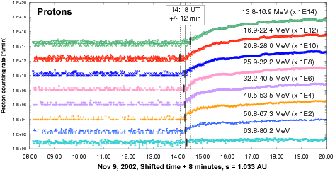
Figure 1.: The proton count rates observed by SOHO/ERNE. The profiles are shifted back in time assuming the path length of 1.03 AU, acquired from the velocity dispersion fit. The thick short vertical lines represent the onset times on different channels, and the proton release time close to the Sun is marked by a long vertical solid line (dashed vertical lines show the error limits). For visual reasons, the profiles have been scaled suitably, and eight minutes have been added to make them comparable to the electromagnetic observations.

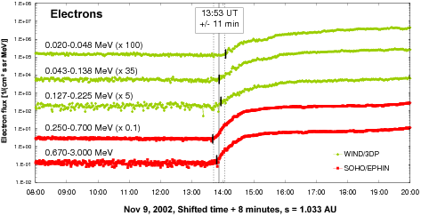
Figure 2.: The shifted electron intensity profiles based on observations by SOHO/EPHIN and Wind/3DP. The applied path length is the same as for protons (1.03 AU). See Figure 1 for details.

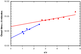
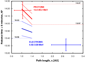
Figure 3.: Fits of the velocity dispersion equation to proton and electron data (top panel). Proton data (triangles) are from the ERNE High Energy Detector HED and electron data (diamonds) from the Wind/3DP and SOHO/EPHIN. Bottom panel shows the estimated release time windows of protons and electrons. Thick inclined lines represent the average proton (red) and electron (blue) release times, when the onset times of several energy channels are shifted back in time with path lengths of 1.0 – 1.4 AU. The time windows (horizontal dashed lines) are based on one standard deviation error limits of the average proton and electron release times (thin inclined lines). The solid crosses represent the results with statistical error limits when the velocity dispersion analysis is carried out separately for proton and electron data.

Using Wind/3DP (0.020 – 0.225 MeV) and SOHO/EPHIN (0.25 – 3.00 MeV) in situ electron observations and assuming the same path length as for the protons, the electron acceleration is estimated to have started at 13:53 UT $\pm$ 11 minutes (Figure 2). However, the path length of 1.03 AU seems to fail in compensating the velocity dispersion of the electron onsets. The velocity dispersion analysis performed only on the electron data yields a very high path length of 2.73 $\pm$ 0.57 AU, which we deem somewhat unreliable (Figure 3). With this high path length the electron release times would have been earlier, at 13:31 UT $\pm$ 8 minutes, but most likely the high value of the path length is caused by an inaccurate determination of the onset times in the low-energy electron channels due to the long rise time and high background level of the fluxes. More conservative estimates of the release time windows are evaluated using path lengths in the 1.0 – 1.4 AU range.

To evaluate the uncertainties in the release times, the standard deviation error limits (1$\sigma$) for the average proton and electron release times were calculated and used to determine the release time windows, as shown in Figure 3. It is clear that protons are delayed with respect to electrons. The delay is much larger if we accept the very high path lengths for the electrons obtained from the velocity dispersion fit to the electron data only. Based on Figure 3, we estimate that the protons in this event were released between 13:57 and 14:27 UT, and the electrons earlier, between 13:40 and 14:03 UT, assuming a low path length for both populations. The electrons could have been released even earlier than that, around 13:23 – 13:39 UT, if a much higher path length is accepted for the electron population.

2.2 CMEs and Flares on 9 November 2002

On 9 November 2002, during the estimated SEP release period, two CMEs were observed. The first (CME1 in Figure 4) was directed to the Northwest. It was first detected at 11:06 UT in LASCO C2, at a height of 2.55 R_⊙, travelling at a plane-of-the-sky speed of 530 km s^-1 (determined from a linear fit to all height-time data points from the LASCO CME Catalog). The second CME (CME2 in Figure 4), was halo-type and directed to the Southwest, and it was first detected at 13:31 UT at a height of 4.20 R_⊙. The plane-of-the-sky speed from a linear fit to all data points was 1840 km s^-1. A second-order fit to the same data points indicates that the halo CME was accelerating, reaching a speed of 2000 km s^-1 near 30 R_⊙. We estimate that the lateral expansion speed (see Schwenn et al., 2005) was even higher than that, about 2300 km s^-1 before 14:00 UT, and about 1800 km s^-1 after 14:00 UT. This speed is, however, difficult to measure, since the northwestern CME2 edge was irregular and varying in time. The three consecutive LASCO C2 difference images in Figure 4 show how the two CMEs evolved and how the halo CME expanded laterally. At 13:54 UT (middle panel in Figure 4) an arc-like brightening is visible between the two CMEs. In the later LASCO C3 images the halo CME surrounds the disk in full 360 degrees.

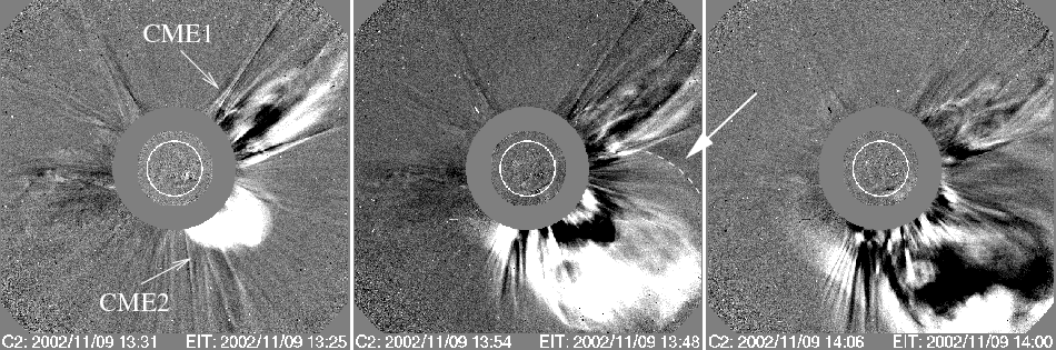
Figure 4.: Evolution of the two CMEs observed on 9 November 2002. The first, directed to the Northwest (CME1), had a plane-of-the-sky speed of about 530 km s^-1. The later halo-type CME (CME2), was directed to the Southwest and had a plane-of-the-sky speed of about 1840 km s^-1. The white dashed line (indicated with an arrow) outlines a brightening on the side of the halo CME at 13:54 UT.

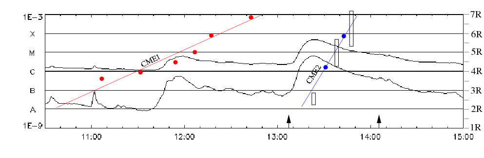
Figure 5.: A height–time plot of the plane-of-the-sky leading fronts of the two CMEs (data from the LASCO CME Catalog) together with the GOES soft X-ray flux curve. Black arrows mark the start times of the RHESSI hard X-ray bursts at 13:07 and 14:05 UT. (Note that RHESSI did not observe during the satellite night-time, between 13:28 and 14:00 UT). Estimated heights for the DH type II burst source are also shown, boxes represent the calculated heights according to the Saito and hybrid density models, see Section 3 for details.

The height–time plot in Figure 5 shows the estimated heights of the CME leading edges, combined with the GOES soft X-ray flux curve during 10:30 – 15:00 UT. The backward-extrapolated height–times for CME2 give an estimated start time for the halo CME near 13:05 UT. The fast halo CME2 was clearly associated with activity in NOAA AR 0180 at S11W36 (location on 9 November at 12:00 UT). The active regions most probably associated with the earlier CME1 were AR 0177 at N18W30 (location on 7 November at 06:30 UT), and AR 0175 at N15W81 (location on 9 November at 15:30 UT ). These active regions are shown in an EIT map on 7 November, in Figure 6. The difference in latitude between the source regions of the two CMEs was 25 – 30^∘ and the difference in longitude 20 – 40^∘, depending on the origin of CME1 (AR 0175 or AR 0177). Since CME2 developed into a full halo and showed lateral expansion, it is possible that the two CMEs made contact. However, as CMEs are observed as projections on the plane of the sky, determining the real geometry is prone to uncertainties.

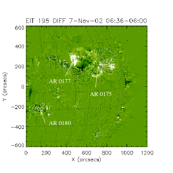
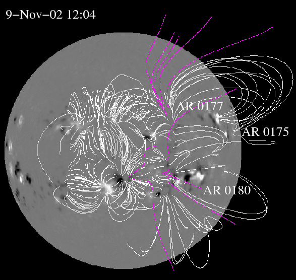
Figure 6.: Top: Active regions associated with the analysed flares and CMEs, observed by SOHO/EIT on 7 November 2002 (difference image at 06:36 – 06:00 UT). By 9 November these regions had rotated about 30^∘ to the West. Bottom: Potential field lines from magnetic field extrapolations (PFSS) using SOHO/MDI magnetogram on 9 November 2002 at 12:04 UT. Field lines plotted in magenta are open, with negative polarity.

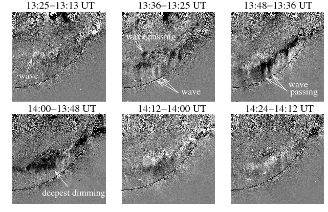
Figure 7.: SOHO/EIT 195 Å difference images showing the EIT wave, wave passing, and dimmings. The shown area is $1000^{\prime\prime}\times 800^{\prime\prime}$ in each frame.

Several GOES C-class flares were recorded during the first CME passage, before 13:00 UT on 9 November, but for many of them the location was not identified. At 13:08 UT a GOES M4.6 class flare started in AR 0180, at S12W29. The flux maximum occurred at 13:23 UT and the flux decayed to the pre-flare level at about 15:00 UT. The timing indicates clear association with the fast halo CME2. RHESSI observed the flare in hard X-rays until 13:28 UT, when satellite night-time set in. The highest energy band in which the flare was observed was 100 – 300 keV. According to the RHESSI flare list the flare was located at $x\,=\,440^{\prime\prime}$, $y\,=\,-264^{\prime\prime}$ from the disk center. After the satellite night-time ended, RHESSI observed an X-ray brightening at 14:05 UT, slightly off from the earlier flare site, at $x\,=\,552^{\prime\prime}$, $y\,=\,-200^{\prime\prime}$.

The potential field (i.e., the current-free field) extrapolations provide an approximation of the magnetic fields in a quiet Sun. However, the lack of electric current and free energy in the model means that it does not describe active regions very well. The PFSS Solarsoft package Schrijver and DeRosa (2003) uses the line-of-sight magnetograms provided by SOHO/MDI, and the potential field in Figure 6 describes the situation on 9 November. On the east side of AR 0180 there are some open field lines (plotted in magenta, indicating negative polarity), and many more in the regions between AR 0180 and AR 0177. It should be noted that the PFSS maps describe the potential field prior to the event, and that ongoing events can strongly perturbe the magnetic structures.

In EUV, coronal loops were observed to open near the nortwest limb at 09:48 UT, at the same latitude where AR 0175 and AR 0177 were located. An EUV brightening appeared in this region at 12:24 UT, and in the following EIT image bright material was ejected over the limb. These transients were observed well before the halo CME2 appeared.

EUV ribbons were formed over the AR 0180 (S12W29) in the EIT image at 13:13 UT, and they were clearly associated with the GOES M4.6 flare. Post-flare loops appeared at 13:25 UT and an EIT wave was observed in the same image. At first it showed as a bright “rim” South of AR 0180, and then as dark dimmed structures near the southwest limb after 13:36 UT (Figure 7). The dark structures persisted well after 14:12 UT. A small EUV brightening was observed in AR 0180 at 14:12 UT, possibly associated with the RHESSI hard X-ray brightening at 14:05 UT.

2.3 Radio Observations

With radio observations we can trace accelerated particles and observe propagating shock fronts. We therefore studied radio emission during 13:00 – 15:00 UT at a large wavelength range (4 GHz – 100 kHz). The dynamic radio spectrum from Artemis-IV at 100 – 600 MHz shows narrow-band fluctuations (nbf) starting around 13:09 UT, one minute after the GOES M4.6 flare start. The fluctuations occured at metric wavelengths, in the 300 – 100 MHz frequency range. The fluctuating envelope drifted slowly towards the lower frequencies (Figure 8). The emission source locations could be imaged by NRH at 164 MHz, and Figure 9 (left panel) shows how the emission centroids were located South of AR 0180, along and over closed loop structures.

Another drifting feature (df) was observed to start around 13:14 UT just below 500 MHz, with a frequency drift around 0.8 MHz s^-1. The dashed lines in Figure 8 mark the frequencies that could be imaged with NRH, and Figure 9 shows the source locations at the three different frequencies. The source trajectory indicates that the burst driver was moving southward from the AR, with a slight path curvature towards the East. We estimate from this image that the projected speed of the emission source was around 1200 – 1400 km s^-1.

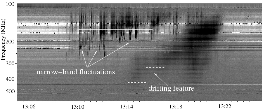
Figure 8.: Artemis-IV spectrum (100 – 600 MHz, 13:05 – 13:25 UT) shows narrow-band fluctuations and a frequency-drifting feature close to the start time of the GOES M4.6 flare. Figure 9 shows some of these source locations, imaged by NRH (times and frequencies are shown here with a white solid line and white dashed lines, respectively). After 13:17:30 UT the features become unclear due to a group of metric type III bursts superposed on the drifting emission.

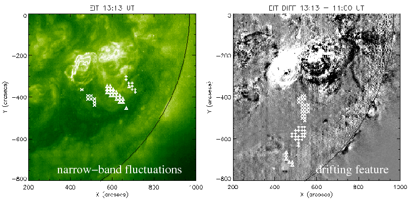
Figure 9.: Left: NRH radio source positions of the narrow-band fluctuations at 164 MHz, plotted over a SOHO/EIT image at 13:13 UT. Right: NRH radio source positions of the drifting burst feature, plotted over a SOHO/EIT difference image 13:13 – 11:00 UT. The emission drifts from 432 MHz (marked with $\times$), through 327 MHz (marked with +), to 236 MHz (marked with $\triangle$). The source positions indicate that the burst driver is moving southward from the AR, with a slight path curvature towards the East. (The imaging periods were indicated in the dynamic spectrum in Figure 8.)

TheWind/WAVES observations at 14 MHz – 20 kHz (Figure 10) show an IP type II burst lane at $\approx$13:20 UT onwards. There is some indication that the burst starts at a frequency higher than the RAD2 upper limit at 14 MHz, as we see emission lanes also around 30 MHz (ground-based observations). During 13:30 – 13:40 UT burst-like emission is observed also at 35 – 65 MHz, and this enhanced emission looks to be separate from the type II burst lane. The type II emission drifts down to 2 MHz by 13:48 UT, when it disappears under the stronger IP type III burst groups. The type II burst lane appears occasionally also after 14:00 UT, and it is seen by WAVES RAD1 at 500 kHz near 15:20 UT.

Several metric–DH type III bursts were observed in association with the main impulsive phase of the M4.6 flare. The first type III burst group that appeared in the estimated time-frame for particle acceleration was observed at 13:28 UT, but the starting frequency is overshadowed by other burst structures. The next group of type III bursts started around 13:48 UT, with starting frequency near $\approx$60 MHz (Figure 10; this frequency was also verified from the DAM dynamic spectrum at 20 – 70 MHz, not shown here). Another type III burst group followed at 14:02 UT. Within this group burst lanes were observed to start at metric wavelengths near 250 MHz at $\approx$14:05 UT (frequency also verified from the Phoenix-2 spectrum).

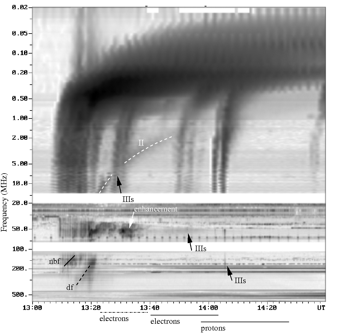
Figure 10.: Composite of radio spectral data at 13:00 – 14:40 UT on 9 November 2002 (Artemis-IV and Wind/WAVES). The narrow-band fluctuations (nbf) and the drifting feature (df) are observed during 13:09 – 13:20 at frequencies higher than 100 MHz (shown in detail in Figure 8). Both of these features could have a continuation at frequencies lower than 70 MHz. At 13:28 – 13:31 UT a type III burst group is observed at DH wavelengths, but the starting frequency is not clear. During 13:30 – 13:40 UT enhanced burst emission is visible at 35 – 65 MHz. Around 13:48 UT a group of type III bursts starts near 60 MHz, followed by another group around 14:05 UT around 250 MHz. An IP type II burst becomes visible around 13:23 UT at 14 MHz. There is some indication that the burst could have started earlier at higher frequencies, but this emission is mixed with type III bursts. The type II emission lane can easily be followed down to 2 MHz near 14:00 UT, when the more intense type III bursts prevent seeing the fainter lane. Estimated electron and proton release times for both path lengths are also marked in the plot. Solid lines represent the release times using 1.0 – 1.4 AU path lengths and dash-dotted line path lengths $>$2.1 AU, see Section 2.1 for details.

On closer inspection, the type III bursts that started near 250 MHz look to be bidirectional. The burst emission drifts both upward and downward in frequency (Figure 11). Bursts with a negative frequency-drift continue to DH wavelengths, while the bursts with a positive drift cannot be identified in the spectrum at frequencies higher than 350 MHz. Negative and positive frequency drifts are usually interpreted as electron beams travelling up and down in the corona, respectively. Some correlation can be found between these bursts and the count-rate peaks recorded by RHESSI in hard X-rays (Figure 11). Since hard X-rays are usually created by downward directed electron beams when they hit denser regions, the type III bursts with a positive frequency drift could be tracing these beams. The type III bursts could be imaged at 327, 236, 164, and 150 MHz by NRH, and the locations along one type III burst are shown in Figure 11. The spatial separation between the RHESSI X-ray burst and the type III burst trajectory indicate that either the sources were separate or the field lines were twisted. However, since the halo CME originated from this same active region, the lateral expansion of the CME could have affected the field lines. We also note the vicinity of the open field lines on the East side of the active region (shown in Figures 6 and 11).

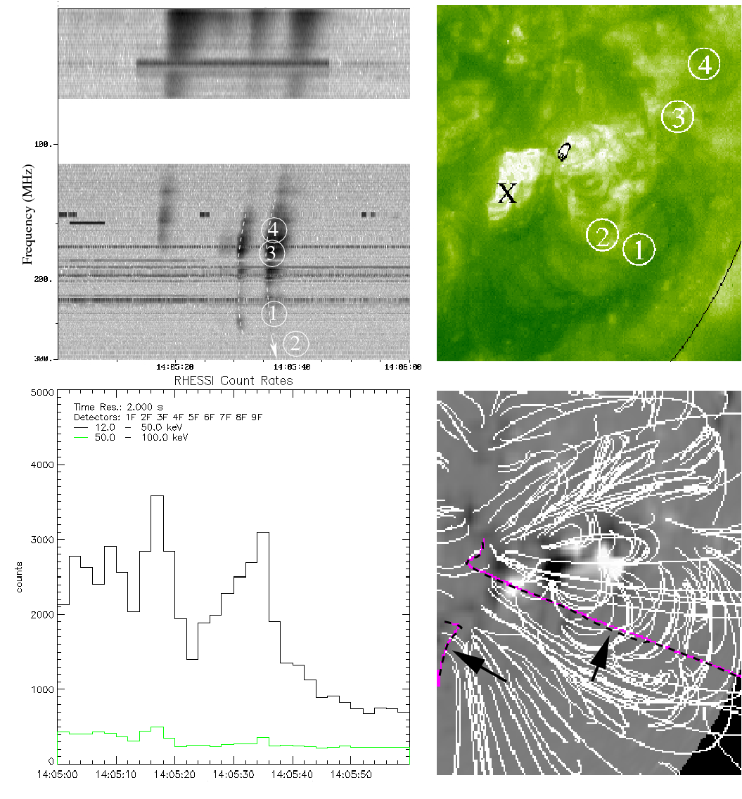
Figure 11.: Top left: Artemis-IV dynamic spectrum at 14:05:00 – 14:06:00 UT at 50 – 300 MHz shows some of the type III bursts in detail. The times and frequencies of the imaged sources 1, 3, and 4, are indicated in the spectrum (burst source 2 at 327 MHz is outside the frequency range shown here). Top right: Emission locations of burst sources 1 – 4. X marks the location of the GOES M4.6 flare with flare maximum at 13:23 UT. Contours show the location of the RHESSI hard X-ray burst at 14:05:00 – 14:06:00 UT. Bottom left: RHESSI count rates from the same time period. Bottom right: Potential magnetic field (PFSS) in the same region as in the top right image, extrapolation is from the SOHO/MDI magnetogram at 12:04 UT on 9 November. Arrows point to the open field-line regions.

All the observed type III bursts continued to DH wavelengths, and the burst lanes look “tilted” at the time when they cross the type II burst lane, see Figure 12. For the 13:48 UT type III burst group the tilt is not so obvious, but there is a brightening in the burst emission. For the 14:05 and 14:40 UT burst groups the type III tilt is more pronounced. It should be noted that in between 14:05 and 14:40 UT, i.e., in the time frame for the estimated proton acceleration, no other burst activity was observed in the dm–DH spectra.

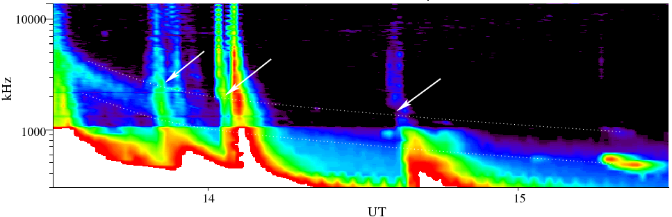
Figure 12.: Wind/WAVES RAD1+RAD2 spectrum at 300 – 14000 kHz at 13:30 – 15:30 UT. The IP type II burst is visible as a patchy, broadband emission lane also after 14:00 UT (band edges outlined with dottted lines). The type III burst groups show a “tilt” at the time of the type II burst passage (times marked with arrows).

3 Radio Source Heights and Velocities

The radio emission during the flare – CME event showed several frequency-drifting structures. As plasma emission is directly related to electron density, $f_{p}$=9000$\sqrt{n_{e}}$ ($n_{e}$ in cm^-3 and $f_{p}$ in Hz), and electron density can be converted to atmospheric height with atmospheric density models, we calculate estimates for the radio source heights. These heights and deduced speeds need to be considered critically, as they depend strongly on the selected density models. Selection of model should be based on the knowledge of coronal conditions in the propagation region, but the available information is often insufficient, see pohjolainen07. Standard coronal density models such as saito70 and newkirk61, and “hybrid” models such as vrsnak04, which is a mixture of the five-fold Saito model for coronal densities and the leblanc98 model for IP densities, can be used to describe the undisturbed high corona at frequencies lower than $\approx$200 MHz (corresponding electron density $n_{e}$ $\lesssim$ 4$\times$10⁸ cm^-3). For the high-frequency emission at 500 – 400 MHz (corresponding electron density $n_{e}$ $\approx$ 2–3$\times$10⁹ cm^-3), we need high-density models such as the ten-fold Saito or a scale height method, to describe densities in active region loops or streamer regions. However, if the exiter of emission is propagating in the wake of earlier transients, in disturbed medium, the height estimates may not give reliable results.

The 300 – 100 MHz frequency range of the burst envelope of the narrow-band fluctuations (nbf) suggests a relatively large height for the emission source already at 13:09 UT. The estimated heliocentric distance at 100 MHz is 1.13 – 1.56 R_⊙, but the actual height value depends strongly on the density model used. From the radio spectrum in Figure 10 it is not clear if the fluctuating emission near 100 MHz is plasma emission at the fundamental frequency or at the second harmonic. Fundamental emission at 50 MHz would place the source height even higher in the corona.

The drifting emission feature (df), observed at 400 MHz around 13:15 UT, had a height of 1.08 R_⊙ according to the 10-fold Saito density model. At 13:17 UT the emission had drifted to 300 MHz, which corresponds to a height of 1.14 R_⊙ using the same model. The deduced burst driver speed is approximately 500 km s^-1. The speed values calculated directly from the atmospheric models assume that the source motion is directed radially against the density gradient, and the speed has to be multiplied by 1/cos($\theta$) if these directions are separated by an angle $\theta$. Usually 45^∘ and multiplication by 1.4 is considered as the realistic maximum correction needed. The scale height method, using the observed $\approx$0.8 MHz s^-1 frequency drift rate, yields a higher speed around 1420 km s^-1. We note that the burst sources of this feature, observed in the NRH images (shown in Figure 9) suggest a projected source velocity of 1200 – 1400 km s^-1, which is close to the value obtained with the scale height method.

The DH type II burst, observed from 14 MHz at 13:23 UT to 2 MHz at 13:47 UT, moved from a heliocentric height of 2.78 R_⊙ to 7.07 R_⊙ (Vršnak, Magdalenić, and Zlopec hybrid density model). The average speed along the burst lane was thus about 2070 km s^-1. Using the Saito density model, instead of the hybrid, the heights are 2.07 and 5.18 R_⊙, with a speed of 1500 km s^-1. In white light, the halo CME front was observed at a height of 5.89 R_⊙ at 13:42 UT, which is closer to the heights calculated with the hybrid density model.

The observed start frequency of the second type III burst group, around 60 MHz near 13:48 UT, suggests that electrons were accelerated near heliocentric distances 1.3 – 1.8 R_⊙ (with all the above-mentioned density models considered). The third type III group started at a much higher frequency, near 250 MHz at 14:05 UT, with bursts that showed both positive and negative frequency drifts. This high frequency indicates a low heliocentric height for acceleration, $<$1.2 R_⊙, with all the density models considered.

4 Results

The sequence of the observed features is listed in Table 1. The narrow-band fluctuations inside the drifting envelope started at 13:09 UT, which is during the flare impulsive phase and also near the time of the estimated halo CME launch time. Radio pulsations can be due to magnetic reconnection, and recently kliem00 have associated this with plasmoid formation. The projected radio sources of this emission were above the active region, which is where the halo CME most probably originated. The source heights for the fluctuations are uncertain, since the observed plasma emission could also reflect the density of the dense active region loops, along which beams of particles were travelling. As the bursts within the envelope had both positive and negative frequency drifts, it is possible that magnetic trapping was present.

The drifting radio feature started next, at 13:14 UT near 500 MHz, which suggests a lower height in the atmosphere compared to the earlier narrow band fluctuations. The estimated speed for the burst driver is difficult to calculate because of the high starting frequency (high frequencies and high densities require that the standard atmospheric models have to be multiplied by arbitrary adjustment factors). From the frequency drift and the density scale height we can make a rough estimate that the speed was around 1420 km s^-1. In the radio images the projected source speed was similar, 1200 – 1400 km s^-1. The source trajectory suggests that this feature could have been associated with the EIT wave. The EIT wave features appeared near the locations of the drifting burst sources at 13:17 UT, near the bright EUV “rim” shown in Figures 7 and 9. Unfortunately we could not calculate the speed of the EIT wave, as it was observed very near the solar limb. The halo CME speed was much higher than the estimated speed of this radio source, and the main halo-CME loop was also moving more to the West compared to the motion of the radio source. The radio source could also be showing a filament trajectory, as the observed EUV ribbons indicated a filament eruption.

Table 1.: Summary of observations related to the 9 November 2002 event

Time (UT)	Event	Comments
09:48 – 12:24	Activity near AR 0175 and AR 0177	loop openings and brightenings
		near the northwestern limb
11:06	Northwestern CME observed	bright front in the Northwest,
		CME speed 530 km s-1
13:08	M4.6 flare onset in AR 0180	GOES, RHESSI
13:09	Narrow-band fluctuations start	frequency range 100 – 300 MHz
13:14	Drifting radio feature starts	start frequency $\approx$500 MHz
13:20	DH type II radio burst observed	at 14 MHz (height 2 – 3 R⊙)
13:23	Flare maximum	GOES
13:23 – 13:39	Electron release time	if path length $>$2.1 AU
13:25	EIT wave observed	bright “rim” south of AR 0180
13:28 – 13:31	Type III burst group	start frequency $<$60 MHz
13:31	Halo CME observed at 4.2 R⊙	bright front in the Southwest
		CME speed 1840 km s-1
13:40 – 14:03	Electron release time	if path length 1.0 – 1.4 AU
13:48 – 13:58	Type III burst group	start frequency $\approx$60 MHz
13:57 – 14:27	Proton release time	if path length 1.0 – 1.4 AU
14:02 – 14:06	Type III burst group	start frequency $\approx$250 MHz
14:05	RHESSI X-ray burst	after satellite night-time
14:12	Deepest EUV dimming

The DH type II burst that we were able to follow from 14 MHz down to 2 MHz, after which it was still observed as patchy emission down to kilometer waves, looks to have a clear association with the CME front. The estimated burst heights fit well with a CME bow shock scenario. The deduced type II burst driver speed at 13:23 – 13:47 UT ($\approx$2070 km s^-1) is not too far off from the plane-of-the-sky CME leading front speed measured at 13:31 – 13:42 UT (1895 km s^-1; acceleration to 2000 km s^-1 near 30 R_⊙) or the measured CME lateral expansion speed, $\approx$2300 km s^-1 before 14:00 UT. The height–time profiles of the type II burst and the CME suggest that both were formed during the flare impulsive phase. A timing match between the flare impulsive phase and the CME acceleration phase have been noted by, e.g., zhang01.

The onset time analysis for protons gives the most probable acceleration time around 13:57 – 14:27 UT. The best candidate for the accelerator is the propagating CME bow shock, visible as the IP type II burst. Near 14:00 UT when the protons could have been released, the (projected) white-light CME front was located at height $\approx$9 R_⊙, and the type II burst height was approximately 7 – 9 R_⊙ (actual number depending on the density model used). We emphasize that between 14:06 and 14:40 UT no other radio signatures were observed in the dynamic spectra.

The two type III burst groups that were observed to start at metric wavelengths (at 60 and 250 MHz) and continued to IP space suggest that electrons were accelerated at low heliocentric heights where they had access to open field lines. Low acceleration heights have been reported earlier by klein05, and their results of acceleration heights were between 0.1 and 0.5 R_⊙ above the photosphere agree with our estimates. They claim that acceleration usually happens well after the flare maximum. The velocity dispersion analysis for the electron data, using the low path length obtained from the proton analysis, gives an estimate for the time of electron release at 13:40 – 14:03 UT. This time range agrees with our observations of the type III burst group observed to start at 13:48 UT. The start of the next type III burst group (14:02 UT) is somewhat late compared with the estimated electron injection time, but it is still possible. Acceleration happens well after the flare maximum (13:23 UT) in this case. But, if we accept the high path length obtained from the analysis of electron data only, the release time (13:23 – 13:39 UT) will match with the flare maximum.

krucker00 have suggested that accelerated electrons can be injected into the Earth-connected flux tube when a coronal transient (EIT wave) hits the field lines. In our case we see the EIT wave passing the southwest “rim” approximately around 13:25 – 13:48 UT, but there is uncertainty due to the poor EIT image cadence. This time frame agrees with the estimated electron injection times with both the low and high path lengths and is close to the start time of the first type III burst group. However, since the origin of EUV emission is relatively low in the solar atmosphere compared to the observed radio emission of the first two type III burst groups, the association remains questionable.

One LASCO image shows that the halo CME had a brightening on the side where the earlier, slower CME was propagating. This brightening appears between the available LASCO C2 images at 13:31 and 13:54 UT. Since the latitudinal and longitudinal distance between the two CME source regions was only 20 – 40^∘, it is possible that the halo CME interacted with the earlier CME or with a streamer located in the northwest. A shock front could have formed in the interaction region, due to compression. The radio enhancement was observed during 13:30 – 13:40 UT at 35 – 65 MHz, where the corresponding heliocentric height is around 1.5 – 2.0 R_⊙. At 13:54 UT the white-light brightening on the CME side had a height of $\approx$4 R_⊙. The deduced speed of the disturbance, if the radio feature and the white-light brigtening were connected, is approximately 1100 – 1500 km s^-1.

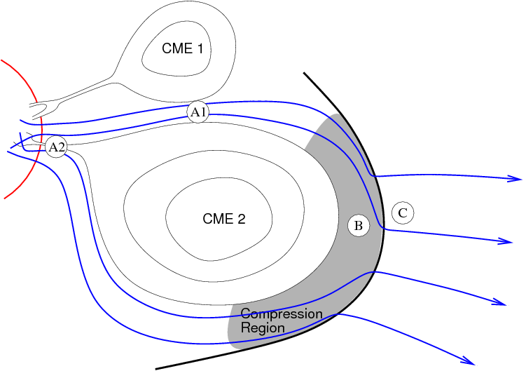
Figure 13.: A sketch of a possible geometry leading to the observed dynamics of the type III bursts: A1 and A2 are the possible reconnection sites where accelerated electrons may have access to open field lines; B is the region where the field lines traverse the compressed region behind the shock front driven by the CME; C is where the density and magnetic field decreases abruptly ahead of the shock, leading to a sudden drop of frequency and the focusing of the electron beam.

We also observed tilted type III burst lanes at times when the type IIIs passed the IP type II burst. After the tilt, some of the type III burst lanes brightened. We present in Figure 13 one possible geometry leading to the observed dynamics. Our sketch also explains the observed bidirectional motion of the metric type III bursts:
– Electrons are accelerated in the possible reconnection site A2 in the low corona, where they have access to open magnetic field lines (some open field lines were present in the potential magnetic field maps prior to the event). The electron beams stream both upwards and downwards, as observed in the dynamic spectra and verified in NRH radio images.
– Site A1 is also a possible reconnection site, because of the open field lines near the active region that produced the earlier CME1/earlier observed streamer region. Since A1 site is located higher in the solar atmosphere than site A2, A1 could be the acceleration region for the second type III burst group (start frequency near 60 MHz) and site A2 could be the the acceleration region for the later birectional type III burst group (start frequency near 250 MHz).
– Accelerated energetic electrons then enter the compression region B which is behind the shock front driven by CME2. The result is a bending of the type III burst lanes as the density gradient along the line of force is diminished. Particles propagate ahead of the shock wave, to region C, and experience a sudden decrease of the local density and magnetic field. This in turn results in a drop of plasma frequency and focusing of the electron beam. The latter, in turn, leads to a more efficient generation of Langmuir waves and, hence, a re-brightening of the radio burst upstream of the shock front.

5 Conclusions

The release times for solar energetic particles, electrons and protons, can be obtained from, e.g., velocity dispersion analysis. The feasibility of this method can be argued, as the path lengths can vary and there can be unknown propagation effects in the IP space. In our analysis protons in the 14 – 80 MeV energy range yield path lengths of 1.0 – 1.4 AU, while the analysed electrons suggest much higher path lengths of 2.4 – 2.7 AU. The path lengths of course have a strong effect on the estimated release times: with the low path lengths, electrons would be released just before the protons, and with adopting the high path lengths just for the electrons, electron release would have preceded proton release by more than half an hour.

Very high path lengths are usually taken as an indication of not-so-accurate timing results (Lintunen and Vainio, 2004; Saiz et al., 2005). High path lengths can be the result of delayed onset observation on low-energy channels due to high pre-event backgrounds, high contrast between the spectral indices of pre-event background and the SEP event, prolonged injection of the particles, or interplanetary scattering of the particles. Therefore the release times yielded by the lower path lengths are more plausible.

We do not speculate on the idea of a “seed population” for the released particles, although there is the possibility of injecting (flare) particles into the corona where the particles get accelerated later. The timing and the high start frequencies of the metric type III bursts that continue to the IP space suggest, however, that at least the energetic electrons are accelerated low in the corona and after the flare maximum.

In summary, from the estimated release times for the electrons and protons compared with the multi-wavelength signatures of flare and coronal mass ejection processes, we conclude that electrons were most probably accelerated at low coronal heights in the wake of a fast halo-type CME – the source region could be reconnecting structures either on the side of the CME or near its legs – and that the best candidate for proton accelerator is the CME bow shock, at a time when the CME was propagating high in the corona, above 9 R_⊙.

The tilts and brightenings in the type III bursts at the times when they pass the IP type II burst is a new observation. We have presented a possible geometry leading to the observed dynamics, and point out that the tilted type III bursts can reveal propagating shock fronts in cases when the type II burst lanes are not visible in the spectrum.

We thank the radio group at LESIA, Observatoire de Paris, France, for the use of Nançay Radioheliograph and Decameter Array data, and the SOHO/EPHIN instrument team and the Wind/3DP instrument team and the Coordinated Data Analysis Web (CDAWeb) for providing the particle data. K-L. Klein and R. Gómez-Herrero are thanked for fruitful discussions. The comments and suggestions made by the anonymous referees improved the paper significantly. The LASCO CME Catalog is generated and maintained by NASA and Catholic University of America in co-operation with the Naval Research laboratory. SOHO is an international co-operation project between ESA and NASA. N.J.L. wishes to thank the Väisälä Foundation of the Finnish Academy of Science and Letters for a travel grant to SPM-11. The Academy of Finland is thanked for partial support under project n:o 104329.

References

- Bougeret et al. (1995) Bougeret, J.-L., Kaiser, M.L., Kellogg, P.J., Manning, R., Goetz, K., Monson, S.J., et al.: 1995, Space Sci. Rev. 71, 231.
- Brueckner et al. (1995) Brueckner, G.E., Howard, R.A., Koomen, M.J., Korendyke, C.M., Michels, D.J., Moses, J.D., et al.: 1995, Solar Phys. 162, 357.
- Cane and Erickson (2005) Cane, H.V., Erickson, W.C.: 2005, Astrophys. J. 623, 1180.
- Cane, Reames, and von Rosenvinge (1988) Cane, H.V., Reames, D.V., von Rosenvinge, T.T.: 1988, J. Geophys. Res. 93, 9555.
- Cliver, Webb, and Howard (1999) Cliver, E.W., Webb, D.F., Howard, R.A.: 1999, Solar Phys 187, 89.
- Dalla et al. (2003) Dalla, S., Balogh, A., Krucker, S., Posner, A., Müller-Mellin, R., Anglin, J. D., et al.: 2003, Ann. Geophys. 21, 1367.
- Debrunner, Flueckiger, and Lockwood (1990) Debrunner, H., Flueckiger, E.O., Lockwood, J. A.: 1990, Astrophys. J. Suppl. Ser. 73, 259.
- Delaboudinière et al. (1995) Delaboudinière, J.-P., Artzner, G.E., Brunaud, J., Gabriel, A.H., Hochedez, J.F., Millier, F., et al.: 1995, Solar Phys. 162, 291.
- Dulk (1985) Dulk, G.A.: 1985, Ann. Rev. Astron. Astrophys. 23, 169.
- Gopalswamy et al. (2002) Gopalswamy, N., Yashiro, S., Michałek, G., Kaiser, M.L., Howard, R.A., Reames, D.V., Leske, R., von Rosenvinge, T.: 2002, Astrophys. J. 572, 103.
- Gosling (1997) Gosling, J.T.: 1997, In: Crooker, N., Joselyn, J.A., Feynman, J. (eds.), Coronal Mass Ejections, Geophysical Monograph 99, American Geophysical Union, Washington, 9.
- Hilchenbach et al. (2003) Hilchenbach, M., Sierks, H., Klecker, B., Bamert, K., Kallenbach, R.: 2003, In: Velli, M., Bruno, R., Malara, F., Bucci, B. (eds.), Solar Wind Ten, AIP Conf. Proc. 679, American Institute of Physics, New York, 106.
- (13) Huttunen-Heikinmaa, K., Valtonen, E., Laitinen, T.: 2005, Astron. Astrophys. 442, 673.
- de Jager (1986) de Jager, C.: 1986, Space Sci. Rev. 44, 43.
- Kahler (1994) Kahler, S: 1994, Astrophys. J. 428, 837.
- Kahler (2003) Kahler, S.W.: 2003, Adv. Space Res. 32, 12, 2587.
- Kallenrode (1993) Kallenrode, M.: 1993, J. Geophys. Res. 98, 5573.
- Kerdraon and Delouis (1997) Kerdraon, A., Delouis, J.: 1997, In: Trottet, G. (ed.), Coronal Physics from Radio and Space Observations, Lecture Notes in Physics 483, Springer-Verlag, Berlin Heidelberg, 192.
- Klein et al. (1999) Klein, K.-L., Chupp, E.L., Trottet, G., Magun, A., Dunphy, P.P., Rieger, E., Urpo, S.: 1999, Astron. Astrophys. 348, 271.
- Klein and Posner (2005) Klein, K.-L., Posner, A.: 2005, Astron. Astrophys. 438, 1029.
- Klein and Trottet (2001) Klein, K.-L., Trottet, G.: 2001, Space Sci. Rev. 95, 215.
- Kliem, Karlicky, and Benz (2000) Kliem, B., Karlicky, M., Benz, A.O.: 2000, Astron. Astrophys. 360, 715.
- Kocharov and Torsti (2002) Kocharov, L., Torsti, J.: 2002, Solar Phys. 207, 149.
- Kontogeorgos et al. (2006) Kontogeorgos, A., Tsitsipis, P., Caroubalos, C., Moussas, X., Preka-Papadema, P., Hilaris, A., Petoussis, V., Bouratzis, C., Bougeret, J.-L., Alissandrakis, C.E., Dumas, G.: 2006, Exp. Astron. 21, 41.
- Krucker et al. (1999) Krucker, S., Larson, D.E., Lin, R.P., Thompson, B.J.: 1999, Astrophys. J. 519, 864.
- Krucker and Lin (2000) Krucker, S., Lin, R.P.: 2000, Astrophys. J. 542, L61.
- Leblanc, Dulk, and Bougeret (1998) Leblanc, Y., Dulk, G.A., Bougeret, J-L.: 1998, Solar Phys. 183, 165.
- Leblanc et al. (2001) Leblanc, Y., Dulk, G.A., Vourlidas, A., Bougeret, J-L.: 2001, J. Geophys. Res. 106, 25301.
- Lecacheux (2000) Lecacheux, A.,: 2000, In: Stone, R.G., Weiler, K.W., Goldstein, M.L., Bougerot J.-L. (eds.), Radio Astronomy at Long Wavelengths, AGU Monograph Series 119, American Geophysical Union, Washington, 321.
- Lin et al. (1995) Lin, R.P., Anderson, K.A., Ashford, S., Carlson, C., Curtis, D., Ergun, R., et al.: 1995, Space Sci. Rev. 71, 125.
- Lin et al. (2002) Lin, R.P., Dennis, B.R., Hurford, G.J., Smith, D.M., Zehnder, A., Harvey, P.R., et al.: 2002, Solar Phys. 210, 3.
- Lintunen and Vainio (2004) Lintunen J., Vainio R.: 2004, Astron. Astrophys. 420, 343.
- Mann et al. (2003) Mann, G., Klassen, A., Aurass, H., Classen, H-T.: 2003, Astron. Astrophys. 400, 329.
- Messmer, Benz, and Monstein (1999) Messmer, P., Benz. A.O., Monstein, C.: 1999, Solar Phys. 187, 335.
- Mewaldt et al. (2003) Mewaldt, R., Cohen, C., Haggerty, D., Gold, R.E., Krimigis, S.M., Leske, R.A., et al.: 2003, In: Kajita, T., Asaoka, Y., Kawachi, A., Matsubara, Y., Sasaki, M. (eds.), Proc. 28th Int. Cosmic Ray Conference 6, Universal Academy Press, Trukuba, 3313.
- Müller-Mellin et al. (1995) Müller-Mellin, R., Kunow, H., Fleissner, V., Pehlke, E., Rode, E., Roschmann, N., et al.: 1995, Solar Phys. 162, 483.
- Nelson and Melrose (1985) Nelson, G.J., Melrose, D.B.: 1985, In: McLean, D.J., Labrum, N.R. (eds.), Solar Radio Physics, Cambridge Univ. Press, Cambridge, 333.
- Newkirk (1961) Newkirk, G. Jr.: 1961, Astrophys. J. 133, 983.
- Pohjolainen et al. (2007) Pohjolainen, S., van Driel-Gesztelyi, L., Culhane, J.L., Manoharan, P.K., Elliott, H.A.: 2007, Solar Phys. 244, 167.
- Reames (1999) Reames, D.V.: 1999, Space Sci. Rev. 90, 413.
- Saito (1970) Saito, K.: 1970, Ann. Tokyo Astr. Obs 12, 51.
- Sáiz et al. (2005) Sáiz, A., Evenson, P., Ruffolo, D., Bieber, J. W.: 2005, Astrophys. J. 626, 1131.
- Scherrer et al. (1995) Scherrer, P.H., Bogart, R.S., Bush, R.I., Hoeksema, J.T., Kosovichev, A.G., Schou, J., et al.: 1995, Solar Phys. 162, 129.
- Schrijver and DeRosa (2003) Schrijver, C.J., DeRosa, M.L.: 2003, Solar Phys. 212, 165.
- Schwenn et al. (2005) Schwenn, R., dal Lago, A., Huttunen, E., Gonzalez, W.D.: 2005, Ann. Geophys. 23, 1033.
- Simnett (2005) Simnett, G.M.: 2005, Solar Phys. 229, 213.
- Torsti et al. (1998) Torsti, J., Anttila, A., Kocharov, L., Mäkelä, P., Riihonen E., Sahla, T., et al.: 1998, Geophys. Res. Lett. 25, 2525.
- Torsti et al. (1995) Torsti, J., Valtonen, E., Lumme, M., Peltonen, P., Eronen, T., Louhola, M., et al.: 1995, Solar Phys. 162, 505.
- Tylka et al. (2003) Tylka, A.J., Cohen, C.M.S., Dietrich, W.F., Krucker, S., McGuire, R.E., Mewaldt, R.A., et al.: 2003, In: Kajita, T., Asaoka, Y., Kawachi, A., Matsubara, Y., Sasaki, M. (eds.), Proc. 28th Int. Cosmic Ray Conference 6, Universal Academy Press, Trukuba, 3305.
- Vilmer et al. (2003) Vilmer, N., Pick, M., Schwenn, R., Ballatore, P., Villain, J.P.: 2003, Ann. Geophys. 21, 847.
- Vršnak, Magdalenić, and Zlopec (2004) Vršnak, B., Magdalenić, J., Zlopec, P.: 2004, Astron. Astrophys. 413, 753.
- Wang et al. (2005) Wang, Y., Zheng, H., Wang, S., Pe, Y.: 2005, Astron. Astrophys. 434, 309.
- Wild (1950) Wild, J. P.: 1950, Aust. J. Sci. Res. A 3, 541.
- Zhang et al. (2001) Zhang, J., Dere, K.P., Howard, R.A., Kundu, M.R., White, S.M.: 2001, Astrophys. J. 559, 452.