Light scalars as tetraquarks: decays and mixing with quarkonia

Francesco Giacosa

Institut für Theoretische Physik
Universität Frankfurt
Johann Wolfgang Goethe - Universität
Max von Laue–Str. 1
60438 Frankfurt, Germany

The tetraquark assignement for light scalar states below 1 GeV is discussed on the light of strong decays. The next-to-leading order in the large-N expansion for the strong decays is considered. Mixing with quarkonia states above 1 GeV is investigated within a chiral approach and the inclusion of finite-width effects is taken into account.

1 Introduction

The nature of scalar states, under debate since over 30 years, represents one of the major problems of low energy QCD, see [1] for reviews. In these proceeding, based on the works [2, 3, 4], the tetraquark hypothesis for the light scalar mesons is discussed.

The resonances $a_{0}(980),$ $f_{0}(980)$ and $f_{0}(600)$ are well established [5] and evidence for the state $k(800),$ although not yet decisive, is mounting. Thus, a full nonet emerges below 1 GeV. Why not to interpret it as a quarkonium scalar nonet? Some serious problems are well known: (a) the mass degeneracy of $a_{0}^{0}(980)$ and $f_{0}(980)$, which would be $\sqrt{1/2}(\overline{u}u-\overline{d}d)$ and $\overline{s}s$ in the $\overline{q}q$ assignment, is unexplained. (b) The coupling of $a_{0}(980)$ to $\overline{K}K$ is large and points to a hidden s-quark component. (c) Scalar quarkonia are p-wave (and spin 1) states, therefore expected to lie above 1 GeV as the tensor and axial-vector mesons. (d) Quenched lattice results [6] find a quarkonium isospin 1 mass $M_{u\overline{d}}=1.4$-$1.5$ GeV, thus showing that $a_{0}(1450),$ rather than $a_{0}(980)$, is the lowest scalar $I=1$ quarkonium; recent unquenched results of Ref. [7] which find in addition to $a_{0}(1450)$ also $a_{0}(980)$, are discussed in the conclusions. (e) In the large-$N_{c}$ study of Ref. [8] it is shown that the resonance $f_{0}(600)$ does $not$ behave as a quarkonium or a glueball state: the width does not scale as $1/N_{c}$ and the mass is not constant.

These problems can be solved in the framework of the tetraquark assignment of the light scalars: as shown by Jaffe 30 years ago [9], when composing scalar diquarks in the color and flavor antitriplet configuration (good diquarks) instead of quarks, the resonance $f_{0}(980)$ is dominantly “$\overline{s}s(\overline{u}u+\overline{d}d)$” and the neutral isovector $a_{0}(980)$ as “$\overline{s}s(\overline{u}u-\overline{d}d)$”, thus neatly explaining the problem (a) mentioned above. The $f_{0}(600)$ is the lightest state with dominant contribution of “$\overline{u}u\overline{d}d$”, in between one has the kaonic state $k(800)$ ($k^{+}$ interpreted as “$\overline{d}d\overline{s}u$”): the mass pattern is nicely reproduced. This is still one of the most appealing properties of the tetraquark assignment. Support for the existence of Jaffe’s states below 1 GeV is also in agreement with the Lattice studies of Refs. [10]. Concerning the other problems mentioned above: (b) is solved because $a_{0}(980)$ has a hidden s-quark content. Points (c) and (d) are solved setting the quarkonia states above 1 GeV: $a_{0}(1450)$ and $K(1430)$ are the isovector and isodoublet respectively, $f_{0}(1370)$, $f_{0}(1500)$ and $f_{0}(1710)$ are the isoscalar states with glueball’s intrusion (with $f_{0}(1500)$ being a hot candidate) [11]. Point (e) is solved in virtue of the large-$N_{c}$ counting for tetraquarks: widths and masses increase for increasing $N_{c}$ [12].

In the following we concentrate on quantitative aspects of the tetraquark assignment: in Section 2 the Clebsch-Gordan coefficients for the strong decays are studied, in Section 3 the inclusion of mixing with quarkonia states is investigated within a chiral approach; subsequently, the inclusion of mesonic loops and finite-width effects is analyzed. Finally, in Section 4 the conclusions are presented.

2 Strong decays in a $SU_{V}(3)$-invariant approach

In the original work of Jaffe [9] the decay of tetraquark states takes place via the so-called superallowed OZI-mechanism (Fig. 1.a): the switch of a quark and an antiquark generates the fall-apart of the tetraquark into two mesons. This mechanism is dominant in the large-$N_{c}$ counting. Already in [9] the possibility that a quark and an antiquark annihilate is mentioned in relation to isoscalar mixing but is not explicitly evaluated for the decay rates. The fact that only one intermediate transverse gluon is present, see Fig. 1.b, may indicate that this mechanism, although suppressed of a factor $1/N_{c}$, is relevant. In [13] the discussion of strong decays of tetraquarks is revisited. Mechanism of Fig. 1.b is mentioned in the end of the work but is not systematically evaluated for all decay modes. This has been the motivation of [2], where the inclusions of both decay modes of Fig. 1.a and Fig. 1.b in a $SU_{V}(3)$-invariant interaction Lagrangian parameterized by two coupling constants $c_{1}$ and $c_{2}$, is performed in all decay channels.

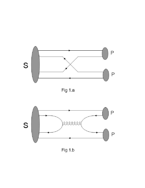
Figure 1: Dominant (1.a) and subdominant (1.b) contributions to the transition amplitudes of a scalar tetraquark state into two pseudoscalar mesons.

The nonet of scalar tetraquark is described by the matrix [2]:

$$\mathcal{S}^{[4q]} \equiv \frac{1}{2}\left(\begin{array}[]{ccc}[\overline{d},\overline{s}][d,s]&-[\overline{d},\overline{s}][u,s]&[\overline{d},\overline{s}][u,d]\\ -[\overline{u},\overline{s}][d,s]&[\overline{u},\overline{s}][u,s]&-[\overline{u},\overline{s}][u,d]\\ [\overline{u},\overline{d}][d,s]&-[\overline{u},\overline{d}][u,s]&[\overline{u},\overline{d}][u,d]\end{array}\right)$$ (4)

$$= \left(\begin{array}[]{ccc}\sqrt{\frac{1}{2}}(f_{B}-a_{0}^{0}(980))&-a_{0}^{+}(980)&k^{+}\\ -a_{0}^{-}(980)&\sqrt{\frac{1}{2}}(f_{B}+a_{0}^{0}(980))&-k^{0}\\ k^{-}&-\overline{k}^{0}&\sigma_{B}\end{array}\right)$$ (8)

where the notation $[u,d]$ refers to the scalar diquark with flavor antysymmetric wave function $(ud-du).$ Thus, the tetraquark composition of the light scalars is directly readable from Eqs. (4)-(8). A mixing of the isoscalar tetraquark states $\sigma_{B}[4q]\equiv\sigma_{B}$ and $f_{B}[4q]\equiv f_{B}$, leading to the physical states $f_{0}(600)$ and $f_{0}(980)$, occurs [2]. The pseudoscalar nonet is contained in the usual matrix $\mathcal{P}=\frac{1}{\sqrt{2}}\sum_{i=0}^{8}P^{i}\lambda_{i}$. The parity, charge conjugation and flavor invariant interaction term reads

$$\mathcal{L}_{\mathcal{S}^{[4q]}PP}=c_{1}\mathcal{S}_{ij}^{[4q]}Tr\left[A^{j}\mathcal{P}^{t}A^{i}\mathcal{P}\right]-c_{2}\mathcal{S}_{ij}^{[4q]}Tr\left[A^{j}A^{i}\mathcal{P}^{2}\right]$$ (9)

with  $\left(A^{i}\right)_{jk}=\varepsilon_{ijk}$. The first term, proportional to $c_{1}$, describes the dominant, fall-apart (OZI-superallowed mechanism) of Fig. 1.a and the second term, proportional to $c_{2}$, the subdominant mechanism of Fig. 1.b.

The decay rates for the channel $S\rightarrow P_{1}P_{2}$ ($S$ stands for scalar, $P$ for pseudoscalar) in the tree-level approximation reads

$$\Gamma_{S\rightarrow P_{1}P_{2}}=\frac{p_{S\rightarrow P_{1}P_{2}}}{8\pi M_{S}^{2}}g_{SP_{1}P_{2}}^{2},$$ (10)

where $p_{S\rightarrow P_{1}P_{2}}$ is the three-momentum of (one of) the outgoing particle(s). The coupling constants $g_{SP_{1}P_{2}}$ are function of the decay constants $c_{1}$ and $c_{2}$ (symmetry factors included). Formula (10) is strictly valid only for narrow states with $M_{S}>>M_{P_{1}}+M_{P_{2}};$ it serves, however, as a useful mnemonic for the used conventions. The amplitude $g_{SP_{1}P_{2}}$ characterizes the strength in a given channel and can be (in principle) extracted directly from experiment. While full values are still unclear, ratios of coupling constants are more stable. In particular, in [14] the following ratio is reported:

$$\frac{g_{f_{0}(980)\overline{K}K}^{2}}{g_{a_{0}(980)\overline{K}K}^{2}}=2.15\pm 0.4.$$ (11)

The theoretical amplitudes in the $\overline{K}K$ channel for $f_{B},$ which in the limit of zero mixing angle coincides with $f_{0}(980)$, and $a_{0}(980)$ as extracted from Eq. (9) read:

$$g_{f_{B}\overline{K}K} = \sqrt{2}\left(\sqrt{2}c_{1}+\frac{3}{\sqrt{2}}c_{2}\right),$$ (12)

$$g_{a_{0}(980)\overline{K}K} = \sqrt{2}\left(\sqrt{2}c_{1}+\frac{1}{\sqrt{2}}c_{2}\right).$$ (13)

If $c_{2}=0$ the ratio $g_{f_{B}\overline{K}K}^{2}/g_{a_{0}(980)\overline{K}K}^{2}$ is 1 and thus not in agreement with Eq. (11). When including mixing in the isoscalar sector, which however should be small in order not to spoil the mass degeneracy of $a_{0}(980)$ and $f_{0}(980)$, the situation is worsened: the ratio turns out to be smaller than 1.

On the contrary, one can notice that the subdominant decay mechanism enhances $g_{f_{B}\overline{K}K}$ more than $g_{a_{0}(980)\overline{K}K}.$ Even a relatively small $c_{2}$ can account for the value in Eq. (11). In [2] a fit to ratios of coupling constants allowed to fix (in a possible mixing scenario) $c_{2}/c_{1}=0.62,$ smaller than $1$ but slightly larger than $1/N_{c}=1/3.$ It is however important to say that within the mentioned fit the coupling of $f_{0}(600)$ to $\overline{K}K$ turns out to be small, while it is found to be sizable in [14]. We refer to [2] for a more detailed analysis of admissible solutions, but more work is needed. For instance, fits to the line shapes of $\phi$ decays (even using different parametrizations than the kaon loop model, see for instance Ref. [15] and Refs. therein) should be performed with new data from KLOE experiment [16]. If the ratio (11) shall be confirmed, the inclusion of the subdominant decay mode is necessary for tetraquark picture of light scalars.

3 Going further: mixing and loops

3.1 Mixing of tetraquark and quarkonia states in a chiral approach

Assuming a nonet of tetraquark states below 1 GeV, mixing with a nonet of quarkonia (with glueball) above 1 GeV takes place and the physical states turn out to be an admixture of a tetraquark and a quarkonium. Thus, in this sense the identification of Eq. (4) with Eq. (8) is not valid any longer.

A crucial point is to estimate the intensity of tetraquark-quarkonia mixing [3]. If it is large, the study of decays and branching ratios is largely influenced and the attempt to explain some phenomenological features, such as the ratio of coupling constants, with only one dominant assignment cannot be correct and both components shall be considered. On the contrary, if it is small it is possible to perform, for instance, the study of the previous section.

In order to study the mixing of tetraquark and quarkonia we have to enlarge the symmetry group. Instead of only $SU_{V}(3)$ invariance as in Eq. (9), full chiral symmetry $SU_{V}(3)\times SU_{A}(3)$ has to be considered. Let us introduce, together with the pseudoscalar quarkonia nonet matrix $\mathcal{P},$ the scalar quarkonia nonet matrix $\mathcal{S}^{[\overline{q}q]}$. We will concentrate on non-isosinglet channels, thus we can disregard the glueball in the following. As usual the complex matrix $\Sigma=\mathcal{S}^{[\overline{q}q]}+i\mathcal{P}$ is introduced. The following chiral Lagrangian

$$\mathcal{L}_{\Sigma}=\frac{1}{4}Tr\left[\partial_{\mu}\Sigma\partial^{\mu}\Sigma^{{\dagger}}\right]-V_{0}(\Sigma,\Sigma^{{\dagger}})-V_{SB}(\Sigma,\Sigma^{{\dagger}})$$ (14)

($Tr$ denotes trace over flavor) describes the dynamics of the pseudoscalar and scalar quarkonia mesons, where $V_{0}$ represents the chiral invariant potential while $V_{SB}$ encodes symmetry breaking due to the non-zero current quark masses. It is important to stress that we do $not$ need to know the potentials $V_{0}$ and $V_{SB}$. What is important for us is simply that spontaneous chiral symmetry breaking ($\chi SB$) occurs. The minimum $\Sigma_{0}$ of the potential $V_{0}+V_{SB}$ is non-zero and is given in a model independent way by the following vacuum expectation values ($vev$’s) [17, 18]:

$$\Sigma_{0}=diag\left\{\frac{F_{\pi}}{\sqrt{2}},\frac{F_{\pi}}{\sqrt{2}},\sqrt{2}F_{K}-\frac{F_{\pi}}{\sqrt{2}}\right\}=diag\left\{\alpha_{u},\alpha_{u},\alpha_{s}\right\}$$ (15)

where $F_{\pi}$ and $F_{K}$ are the pion and kaon decay constants.

The full chirally invariant interaction Lagrangian involves not only scalar, but also pseudoscalar diquarks [3]. The latter are however more massive and less bound [19]. Retaining only the scalar ‘good’ diquarks, the interaction Lagrangian, connecting the tetraquark nonet $\mathcal{S}^{[4q]}$ to the quarkonia states $\Sigma=\mathcal{S}^{[\overline{q}q]}+i\mathcal{P}$ and taking into account diagrams of the type of Fig. 1.a and 1.b, turns out to be [3]:

$$\mathcal{L}_{\mathcal{S}^{[4q]}\Sigma\Sigma}=-\frac{c_{1}}{2}\mathcal{S}_{ij}^{[4q]}Tr\left[A^{j}\Sigma^{t}A^{i}\Sigma+D\Sigma^{\ast}D^{\dagger}\Sigma^{\dagger}\right]-\frac{c_{2}}{2}\mathcal{S}_{ij}^{[4q]}Tr\left[A^{j}A^{i}\Sigma^{\dagger}\Sigma+A^{j}A^{i}\Sigma\Sigma^{\dagger}\right].$$ (16)

Notice that the coupling constants $c_{1}$ and $c_{2}$ are the same of the previous section: in fact, $\mathcal{L}_{\mathcal{S}^{[4q]}PP}$ of Eq. (9) is entirely contained $\mathcal{L}_{\mathcal{S}^{[4q]}\Sigma\Sigma}.$ When expanding around the minimum $\Sigma_{0}$ of Eq. (15) mixing among scalar tetraquark and quarkonia arises: the mixing strength in a given channel is then a combination of the two couplings $c_{1},$ $c_{2}$ and the decay constants $F_{\pi},$ $F_{K}.$ Thus, using experimental informations on decay widths of scalar states from PDG [5], which constraints $c_{1}$ and $c_{2},$ we can estimate the intensity of mixing. Let us make a concrete example in the neutral isovector channel $I=1$. The mixing term emerging from the interaction Lagrangian (16) and from equation (15) reads

$$\mathcal{L}_{\mathcal{S}^{[4q]}\Sigma\Sigma}\rightarrow\mathcal{L}_{mixa_{0}^{0}}=2(c_{1}\alpha_{s}+c_{2}\alpha_{u})\left(a_{0}^{0}[4q]\cdot a_{0}^{0}[\overline{q}q]\right)$$ (17)

where $a_{0}^{0}[4q]=\frac{1}{2}([\overline{u},\overline{s}][u,s]-[\overline{d},\overline{s}][d,s])$ refers to a bare tetraquark state and $a_{0}^{0}[\overline{q}q]=\frac{1}{\sqrt{2}}(\overline{u}u-\overline{d}d)$ to the quarkonium. The physical resonances $a_{0}(980)$ and $a_{0}(1450)$ are then an admixture of the bare components:

$$\left(\begin{array}[]{c}a_{0}^{0}(980)\\ a_{0}^{0}(1470)\end{array}\right)=\left(\begin{array}[]{cc}\cos(\theta)&\sin(\theta)\\ -\sin(\theta)&\cos(\theta)\end{array}\right)\left(\begin{array}[]{c}a_{0}^{0}[4q]\\ a_{0}^{0}[\overline{q}q]\end{array}\right).$$ (18)

Bounds on the full decay widths from PDG allow us to reach the conclusion $(\sin\theta)^{2}<10\%,$ that is the mixing angle is small, see details in [3]. The state $a_{0}^{0}(980)\simeq a_{0}^{0}[4q]$ is dominantly a tetraquark and $a_{0}^{0}(1470)\simeq a_{0}^{0}[\overline{q}q]$ a quarkonium. A similar result holds for the kaonic states, see however also the different outcome in [20]. In turn, this means that identifying Eq. (4) with Eq. (8), as done in the previous section, is correct in first approximation. Notice moreover that these results depend only very weakly on the ratio $c_{2}/c_{1}.$

A note of care concerning the isoscalar sector, where a direct mixing of 5 states takes place (two tetraquarks two quarkonia and one glueball), is needed . While results are consistent with a substantial separation of tetraquark form quarkonia (plus glueball) states, my point of view is that experimental information is not yet good enough to unequivocally extract the mixing angles.

As a last step we mention the results concerning the emerging of a tetraquark condensate: the field $\sigma_{B}[4q]$, referring to $\frac{1}{2}[\overline{u},\overline{d}][u,d]$ and introduced in Eqs. (4) and (8), acquires a nonzero $vev$ [3]:

$$\left\langle\sigma_{B}[4q]\right\rangle=\frac{c_{1}+c_{2}}{M_{\sigma_{B}[4q]}^{2}}F_{\pi}^{2}$$ (19)

where $M_{\sigma_{B}[4q]}\simeq 0.6$ GeV. Notice that this $vev$ vanishes if $F_{\pi}\rightarrow 0,$ i.e. if the quark condensate is zero: the tetraquark condensate is induced by the quark condensate in this framework. The actual value of the tetraquark condensate can be estimated by introducing $\Lambda_{QCD}\sim 0.25$ GeV as in [17] $\left\langle\frac{1}{2}[\overline{u},\overline{d}][u,d]\right\rangle\sim\Lambda_{QCD}^{5}\left\langle\sigma_{B}[4q]\right\rangle\simeq 3.1\cdot 10^{-5}$ GeV⁶.

3.2 Mesonic loops

All the considerations up to now were based on the tree-level approximation. The inclusion of mesonic loops and finite-width effects is the next step in the study of decays of light scalars [4]. Be the propagator of a scalar state $S$ the function $\Delta_{S}(x)=\left(x^{2}-M_{0}^{2}+\Pi(x)+i\varepsilon\right)^{-1}$ where $M_{0}$ is the bare mass, $\Pi(x)$ is the dressing function of mesonic loops (for instance, $\pi\pi$ and $\overline{K}K$ loops contribute for $f_{0}(980)$) and $x=\sqrt{p^{2}}.$ The spectral function is defined as $d_{S}(x)=\frac{2x}{\pi}\lim_{\varepsilon\rightarrow 0}\Delta_{S}(x).$ When the propagator satisfy the Källen-Lehman representation the normalization $\int_{0}^{\infty}d_{S}(x)\mathrm{dx}=1$ is assured [21]. The function $d_{S}(x)$ is the mass-distribution of the scalar state $S.$ The real part of the loop function $\Pi(x)$ is made convergent by ‘delocalizing’ the corresponding interaction Lagrangian by a cutoff function which dies off at a scale of 1.5-2 GeV. All quantities are evaluated in the scheme of a nonlocal Lagrangian and the normalization of $d_{S}(x)$ is a consequence (and a consistency check) of the calculation, see details in [4]. The decay formula (10) modifies as follows:

$$\Gamma_{S\rightarrow P_{1}P_{2}}=\int_{0}^{\infty}\mathrm{dx}\frac{p_{S\rightarrow P_{1}P_{2}}}{8\pi x^{2}}g_{SP_{1}P_{2}}^{2}d_{S}(x)$$ (20)

where the average over the mass-distribution $d_{S}(x)$ is evident. Some comments are in order: (a) the mass of the scalar particle can be defined as the zero of the real part of the propagator, $M^{2}-M_{0}^{2}+$Re$[\Pi(M)]=0$. Typically $M<M_{0},$ i.e. quantum corrections lower the mass. Various definitions of mass (including the widely used position of the pole on the complex plane) are possible. Indeed, the average-mass $\left\langle M\right\rangle=$ $\int_{0}^{\infty}\mathrm{dx}d_{S}(x)x$ can be an intuitive alternative. (b) The width, as evaluated via Eq. (20), is (slightly) smaller than the tree-level counterpart far from threshold. For the $\overline{K}K$ mode of $a_{0}(980)$ and $f_{0}(980)$ it is, on the contrary, sizable while the tree-level decay rate vanishes. (c) The states $a_{0}(980)$ and $f_{0}(980)$ turn out to contain large amount of $\overline{K}K$ clouds, i.e. they spend consistent part of their life as $\overline{K}K$ pairs. On a microscopic level the scalar diquarks are extended objects with a radius of about 0.2-0.5 fm (a small radius is found within the NJL model [22] while a larger one within the BS-approach [23]). Being the typical meson radius of about 0.5-1 fm it is clear that a non-negligible overlap of the two diquarks takes place. As depicted in Fig. 1.a the rearrangement of the two colored bumps (diquark) into two colorless mesons occurs: the system spends consistent part of its life as a mesonic molecular state [24].

Although all these effects are important and deserve further study such as the inclusion of derivative coupling and $a_{0}(980)$-$f_{0}(980)$ mixing effects [25], the scenario as outlined in Section 1 is not qualitatively modified: Clebsch-Gordan coefficients of tree-level amplitudes offer a way to distinguish among different spectroscopic interpretations of the light scalars.

4 Conclusions

In this paper we studied some aspects of the tetraquark interpretation of light scalars: the next to leading order in the large-$N_{c}$ expansion, see Fig. 1.b, has been introduced and its consequences briefly summarized in Section 2 [2]. The decisive point in favour of Fig. 1.b is the ratio [14] $g_{f_{0}(980)\overline{K}K}^{2}/g_{a_{0}(980)\overline{K}K}^{2}=2.15\pm 0.4$. Future studies are needed to extract precisely the values of the coupling constants, thus allowing to compare different assignments for the light scalars.

We then turned the attention to two related phenomena: (a) the mixing of tetraquark and quarkonia states, studied in the framework of a chiral Lagrangian [3]: the results point to a small mixing and to a separation of tetraquark states ($<$ 1 GeV) and quarkonia ($>$ 1 GeV). Noticeably, one does not need to specify the form of the chiral Lagrangian: the requirement of chiral symmetry breaking, together with the experimental information on decay widths from [5], is sufficient to find upper limits for the mixing angles. (b) Mesonic loops and finite-width effects represent an important extension beyond tree-level [4] allowing the evaluation $a_{0}(980)\rightarrow\overline{K}K$ and $f_{0}(980)\rightarrow\overline{K}K$. Both extensions (a) and (b) do not change the qualitative picture emerging in Section 2.

As mentioned in the Introduction in the recent unquenched calculation of [7] the $a_{0}(1450)$ is still present, but a lower state, compatible with $a_{0}(980)$ shows up: however, unquenched lattice calculations $do$ include quark loops and therefore induce also tetraquark admixtures. Indeed, in the ideal limit Lattice simulations should reproduce the physical states regardless of their inner structure. In this sense quenched simulations might be more suitable to answer the question related to the bare quarkonia states: for this reason we still consider valid the results of [6], according to which the bare isovector quarkonium lies in the $1.5$ GeV mass region.

The two-photon mechanism has not been discussed here but will be subject of a forthcoming proceeding, see however [2] and the recent work [26]. Future theoretical studies aiming to understand the nature of light scalars will focus on the following subjects: (i) the radiative decay of $\phi$ meson ($\phi\rightarrow\gamma S\rightarrow\gamma PP)$, in particular concerning the line shapes [16]. (ii) Predictions for scalar decays into a vector meson and a photon ($S\rightarrow V\gamma)$ [27]. (iii) Decays of heavier states, such as $J/\psi$, into light scalars taking into account the tetraquark interpretation of the latter.

References

- [1] C. Amsler and N. A. Tornqvist, Phys. Rept. 389, 61 (2004). F. E. Close and N. A. Tornqvist, J. Phys. G 28, R249 (2002) [arXiv:hep-ph/0204205]; R. L. Jaffe, Phys. Rept. 409 (2005) 1 [Nucl. Phys. Proc. Suppl. 142 (2005) 343] [arXiv:hep-ph/0409065].
- [2] F. Giacosa, Phys. Rev. D 74 (2006) 014028 [arXiv:hep-ph/0605191].
- [3] F. Giacosa, Phys. Rev. D 75 (2007) 054007 [arXiv:hep-ph/0611388].
- [4] F. Giacosa and G. Pagliara, to appear in Phys. Rev. C, arXiv:0707.3594 [hep-ph].
- [5] W. M. Yao et al. [Particle Data Group], J. Phys. G 33 (2006) 1.
- [6] S. Prelovsek, C. Dawson, T. Izubuchi, K. Orginos and A. Soni, ‘ Phys. Rev. D 70 (2004) 094503 [arXiv:hep-lat/0407037]. T. Burch, C. Gattringer, L. Y. Glozman, C. Hagen, C. B. Lang and A. Schafer, Phys. Rev. D 73 (2006) 094505 [arXiv:hep-lat/0601026]. N. Mathur et al., arXiv:hep-ph/0607110.
- [7] R. Frigori, C. Gattringer, C. B. Lang, M. Limmer, T. Maurer, D. Mohler and A. Schafer, arXiv:0709.4582 [hep-lat].
- [8] J. R. Pelaez, Phys. Rev. Lett. 92 (2004) 102001 [arXiv:hep-ph/0309292]. J. R. Pelaez, Mod. Phys. Lett. A 19 (2004) 2879 [arXiv:hep-ph/0411107].
- [9] R. L. Jaffe, Phys. Rev. D 15 (1977) 267. R. L. Jaffe, Phys. Rev. D 15 (1977) 281. R. L. Jaffe and F. E. Low, Phys. Rev. D 19, 2105 (1979).
- [10] M. G. Alford and R. L. Jaffe, Nucl. Phys. B 578 (2000) 367 [arXiv:hep-lat/0001023]. F. Okiharu, H. Suganuma, T. T. Takahashi and T. Doi, arXiv:hep-lat/0601005.
- [11] C. Amsler and F. E. Close, Phys. Lett. B 353, 385 (1995) [arXiv:hep-ph/9505219]; C. Amsler and F. E. Close, Phys. Rev. D 53, 295 (1996) [arXiv:hep-ph/9507326]. W. J. Lee and D. Weingarten, Phys. Rev. D 61, 014015 (2000) [arXiv:hep-lat/9910008]; M. Strohmeier-Presicek, T. Gutsche, R. Vinh Mau and A. Faessler, Phys. Rev. D 60, 054010 (1999) [arXiv:hep-ph/9904461]. F. E. Close and A. Kirk, Eur. Phys. J. C 21, 531 (2001) [arXiv:hep-ph/0103173]. F. Giacosa, T. Gutsche and A. Faessler, Phys. Rev. C 71, 025202 (2005) [arXiv:hep-ph/0408085]. F. Giacosa, T. Gutsche, V. E. Lyubovitskij and A. Faessler, Phys. Rev. D 72, 094006 (2005) [arXiv:hep-ph/0509247]. F. Giacosa, T. Gutsche, V. E. Lyubovitskij and A. Faessler, Phys. Lett. B 622, 277 (2005) [arXiv:hep-ph/0504033].
- [12] R. L. Jaffe, arXiv:hep-ph/0701038.
- [13] L. Maiani, F. Piccinini, A. D. Polosa and V. Riquer, Phys. Rev. Lett. 93 (2004) 212002 [arXiv:hep-ph/0407017].
- [14] D. V. Bugg, Eur. Phys. J. C 47 (2006) 57 [arXiv:hep-ph/0603089].
- [15] N. N. Achasov and A. V. Kiselev, Phys. Rev. D 73 (2006) 054029 [Erratum-ibid. D 74 (2006) 059902] [arXiv:hep-ph/0512047].
- [16] F. Ambrosino et al. [KLOE Collaboration], Eur. Phys. J. C 49 (2007) 473 [arXiv:hep-ex/0609009]. F. Ambrosino et al. [KLOE Collaboration], arXiv:0707.4609 [hep-ex].
- [17] D. Black, A. H. Fariborz, S. Moussa, S. Nasri and J. Schechter, Phys. Rev. D 64 (2001) 014031 [arXiv:hep-ph/0012278].
- [18] S. Gasiorowicz and D. A. Geffen, Rev. Mod. Phys. 41 (1969) 531.
- [19] E. V. Shuryak, Nucl. Phys. B 203 (1982) 93. T. Schafer and E. V. Shuryak, Rev. Mod. Phys. 70 (1998) 323 [arXiv:hep-ph/9610451]. E. Shuryak and I. Zahed, Phys. Lett. B 589 (2004) 21 [arXiv:hep-ph/0310270]. U. Vogl and W. Weise, Prog. Part. Nucl. Phys. 27 (1991) 195. P. Maris and C. D. Roberts, Int. J. Mod. Phys. E 12 (2003) 297 [arXiv:nucl-th/0301049]. Z. Liu and T. DeGrand, PoS LAT2006 (2006) 116 [arXiv:hep-lat/0609038]. D. K. Hong, Y. J. Sohn and I. Zahed, Phys. Lett. B 596 (2004) 191 [arXiv:hep-ph/0403205].
- [20] A. H. Fariborz, R. Jora and J. Schechter, Phys. Rev. D 72 (2005) 034001 [arXiv:hep-ph/0506170]. A. H. Fariborz, Int. J. Mod. Phys. A 19 (2004) 2095 [arXiv:hep-ph/0302133].
- [21] N. N. Achasov and A. V. Kiselev, Phys. Rev. D 70 (2004) 111901 [arXiv:hep-ph/0405128].
- [22] K. Suzuki, T. Shigetani and H. Toki, Nucl. Phys. A 573 (1994) 541 [arXiv:hep-ph/9310266].
- [23] J. C. R. Bloch, C. D. Roberts, S. M. Schmidt, A. Bender and M. R. Frank, Phys. Rev. C 60 (1999) 062201 [arXiv:nucl-th/9907120].
- [24] V. Baru, J. Haidenbauer, C. Hanhart, Yu. Kalashnikova and A. E. Kudryavtsev, Phys. Lett. B 586, 53 (2004) [arXiv:hep-ph/0308129].
- [25] C. Hanhart, B. Kubis and J. R. Pelaez, Phys. Rev. D 76 (2007) 074028 [arXiv:0707.0262 [hep-ph]].
- [26] F. Giacosa, T. Gutsche and V. E. Lyubovitskij, arXiv:0710.3403 [hep-ph].
- [27] Y. Kalashnikova, A. Kudryavtsev, A. V. Nefediev, J. Haidenbauer and C. Hanhart, Phys. Rev. C 73 (2006) 045203 [arXiv:nucl-th/0512028].