Dark Energy and Structure Formation: Connecting the Galactic and Cosmological Length Scales

Abstract

On the cosmological length scale, recent measurements by WMAP have validated $\Lambda$CDM to a precision not see before in cosmology. Such is not the case on galactic length scales, however, where the ‘cuspy-core’ problem has demonstrated our lack of understanding of structure formation. Here, we propose a solution to the ’cuspy-core’ problem based on the observation that with the discovery of Dark Energy, $\Lambda_{DE}$, there is now a universal length scale, $\lambda_{DE}=c/(\Lambda_{DE}G)^{1/2}$, associated with the universe. This length scale allows for an extension of the geodesic equations of motion that affects only the motion of massive test particles; the motion of massless test particles are not affected, and such phenomenon as gravitational lensing remain unchanged. An evolution equation for the density profile is derived, and an effective free energy density functional for it is constructed. We conjecture that the pseudoisothermal profile is preferred over the cusp-like profile because it has a lower effective free energy. A cosmological check of the theory is made using the observed rotational velocities and core sizes of 1393 spiral galaxies. We calculate $\sigma_{8}$ to be $0.68_{\pm 0.11}$; this is within experimental error of the WMAP value $0.761_{-0.048}^{+0.049}$. We then calculate $R_{200}=270_{\pm 130}$ kpc, which is in agreement with observations. We estimate the fractional density of matter that cannot be determined through gravity to be $0.197_{\pm 0.017}$; this is nearly equal to the WMAP value for the fractional density of nonbaryonic matter $0.196^{+0.025}_{-0.026}$. The fractional density of matter that can be determined through gravity is then calculated to be $0.041_{-0.031}^{+0.030}$; this is nearly equal to $\Omega_{B}=0.0416_{-0.0039}^{+0.0038}$.

I Introduction

The recent discovery of Dark Energy (see Riess (1998); Perlmutter (1998) and references therein) has broadened our knowledge of the universe, and has demonstrated once again that it can hold surprises for us. The discovery has, most assuredly, also brought into sharp relief the degree of our understanding of it. Only a small fraction of the mass-energy density of the universe is made up of matter that we have characterized; the rest consists of Dark Matter and Dark Energy, and the precise properties of either one is not known. They are nevertheless needed to explain what is seen on an extremely wide range of length scales. On the galactic ($\sim 100$ kpc parsec), galactic ($\sim$  10 Mpc), and supercluster ($\sim$ 100 Mpc) scales, Dark Matter has been used to explain phenomena ranging from the formation of galaxies and their rotation curves, to the dynamics galaxies and the formation galactic clusters and superclusters. On the cosmological length scale, Dark Matter and Dark Energy is needed to explain the observed evolution of the universe from the Big Bang to the present, and will determine its fate in the future.

Observations thus tell us that over a vast range of length scales the dynamics and evolution of the observed universe is determined not by normal matter, but by Dark Matter and now Dark Energy (see Cahill (2007) for a quantum-cosmology approach that does not require Dark Matter or Dark Energy). Yet while the need and invocation of Dark Matter is ubiquitous on a wide range of length scales, our understanding of how matter determines dynamics at the galactic length scale is lacking. Recent measurements by WMAP Spergal (2007) have validated the $\Lambda$CDM model of cosmology to an precision not seen before in cosmology. The situation on the galactic scale is not nearly as settled, however. Here, the cuspy-core problem for the density profile of matter in galaxies (Navarro (1996); Kravtsov (1998); Moore (1999), and Peebles (2003); Silk (2005) for reviews) has demonstrated our lack of understanding of the formation of galactic rotation curves.

Current understanding of the structure formation is based on the work of Peebles Peebles (1984), where the seeds of galaxies are due to local fluctuations in the density of matter that grow as the universe expands. Analytical solutions of this model have been done Gunn (1972); Fillmore (1984); Hoffman (1985, 1988) for a number of special cases, and have resulted in density profiles that are sensitive to initial conditions, and have a power-law dependence whose exponents vary over a range of values. More recently, numerical simulations Navarro (1996); Kravtsov (1998); Moore (1999) of galaxy formation have been done, and have consistently resulted in density profiles with a cusp-like structure

$$\rho_{\hbox{\scriptsize Simulation}}=\frac{\rho_{i}}{(r/R_{S})^{\gamma}(1+(r/R_{S})^{\alpha})^{(\beta-\gamma)/\alpha}},$$ (1)

instead of the expected pseudoisothermal density profile. Here, $\rho_{i}$ is a density parameter, $R_{s}$ is related to the radius of the galactic core, and the exponents $(\alpha,\beta,\gamma)$ take a range of values from $(1.5,2,1.5)$ for Moore et. al. Moore (1999) to $(1.0,3.0,1.0)$ for Navarro, Frenk and Wilson (NFW) Navarro (1996) (see Silk (2005) for review). This lead Moore to state in Moore (1999) that cold dark matter fails to reproduce the galactic rotation curves for dark-matter-dominated galaxies, one of the key reasons that dark matter was proposed in the first place. Soon afterwards, de Blok and coworkers Blok (2001); deBlok (2002); McGaugh (2001) explicitly demonstrated that the NFW density profile does not fit the density profile observed for Low Surface Brightness (LSB) galaxies (see also Gentile (2007) for a recent analysis of cusp structure). Rather, the traditional pseudoisothermal profile, with $(\alpha,\beta,\gamma)=(2,2,0)$, is the better fit. This demonstration is especially compelling as it is believed that dark matter dominates dynamics in LSB galaxies.

There have been a number of attempts to solving the cuspy-core problem within $\Lambda$CDM Bode (2001); Davé (2001); Sommer-Larsen (2001); Spergal (2000), and they have had varying degrees of success (see Peebles (2003) for a review). This problem does not exist in Milgrom’s Modified Newtonian Dynamics (MOND) Milgrom (1983, 1983, 1983) (see Sanders (2006) for a review)—a theory where Dark Matter is not needed—but there are a number of theoretical and observational problems that MOND must overcome (see Sellwood (2001) for arguments in support of MOND, however).

Our approach to solving the cuspy-core problem, and to structure formation in general, is much more drastic; therefore, its reach is correspondingly broader. It is based on the observation that with the discovery of Dark Energy, $\Lambda_{DE}$, we now have a universal length scale, $\lambda_{DE}=c/(\Lambda_{DE}G)^{1/2}$, on hand . The geodesic equations of motion (GEOM)—and thus the geodesic action—is no longer unique, and extensions of it through the introduction of functions of $Rc^{2}/\Lambda_{DE}G$ can be made. While there have been attempts at proving that the GEOM are the unique consequence of the Einstein field equations Einstein (1938); Geroch (1972, 2006), such proofs assume that the background metric remains fixed under the passage of the test particle. As our extension of the depends explicitly on the energy-momentum tensor of matter—which includes the motion of the test particle—these proofs do not preclude our extension of the GEOM.

In form, our extension of the GEOM preserves the equivalence principal, and through the choice of the function of $Rc^{2}/\Lambda_{DE}G$, we can insure that their effects are not measurable on terrestrial scales. Physically, that this choice is possible is because $\Lambda_{DE}=(7.21^{+0.83}_{-0.84})\hbox{ x }10^{-30}$ $g/cm^{3}$ (from Spergal (2007)) is so much smaller than any density of matter either presently achievable experimentally, or present in regions of space accessible to experiment. Correspondingly, $\lambda_{DE}=14020^{790}_{810}$ Mpc is much longer than the scale of any experiment that has been used to test general relativity. In fact, the issue is to make the theory relevant at galactic scales of a few kpc, and by doing so we arrive at an estimate for the exponent $\alpha_{\Lambda}$. This exponent is the only parameter in the theory, and it determines the power-law behavior of our extension of the GEOM. We also find that while affecting the motion of massive test particles, our extension does not affect the motion of massless test particles; photons still travel along null geodesics, and gravitational lensing and the deflection of light are left unchanged.

Applied to galaxy formation, the extended GEOM reduces to a nonlinear evolution equation for the density profile of a model galaxy in the nonrelativistic, linear gravity limit. This evolution equation minimizes a functional of the density, which is interpreted as an effective free energy functional for the system. Solutions to this equation is found using various velocity curves for galaxies as driving terms, and these solutions are then used to calculate the free energy associated with various profiles. We conjecture that like Landau-Ginzberg phenomenological theories in condensed matter physics, the system prefers to be in a state that minimizes this free energy. Showing that the pseudoisothermal profile is preferred over cusp-like profiles reduces to showing that it has the lower free energy.

In our model of a galaxy, the Hubble length scale $\lambda_{H}=c/H$ (where $H=hH_{0}$, is the Hubble constant, $h=0.732^{+0.031}_{-0.032}$ and $H_{0}=100$ $km/s/$Mpc Spergal (2007)) naturally appears, even though a cosmological model is not mentioned either in its construction or in its analysis. What happens at galactic length scales are naturally tied to what happens at cosmological length scales with our approach; the combination of the Dark Energy length scale and the nonlinear aspects of the extended GEOM link the two. This linkage allows us to extrapolate from the statistical properties of the observed universe the properties of a representative galaxy. These properties are then used to provide a cosmological check of the theory.

As with the Peebles model, the total density of matter for our model galaxy can be written as a sum of a background density $\rho_{\hbox{\scriptsize asymp}}(\mathbf{x})$ and a linear perturbation $\rho_{II}^{1}(\mathbf{x})$. As usual, $\rho_{\hbox{\scriptsize asymp}}(\mathbf{x})$ does not contribute to the motion of stars within the galaxy, while $\rho_{II}^{1}(\mathbf{x})$ does; in the absence of forces other than gravity, observations of the dynamics of the stars will determine only $\rho_{II}^{1}(\mathbf{x})$. But unlike the Peebles model, $\rho_{\hbox{\scriptsize{asymp}}}$ is not a constant. With it, we are able to estimate $\Omega_{\hbox{\scriptsize{asymp}}}$, the fractional density of matter that cannot be determined through gravity, to be $0.197_{\pm 0.017}$; this is nearly equal to the measured value of the fractional density of nonbaryonic (dark) matter in the universe $\Omega_{m}-\Omega_{B}=0.196^{+0.025}_{-0.026}$ measured by WMAP Spergal (2007). Correspondingly, we estimate $\Omega_{\hbox{\scriptsize{Dyn}}}$, the fractional density of matter in the universe that can be determined through gravity, to be $0.041^{+0.030}_{-0.031}$; this is nearly equal to the value of $0.0416^{+0.0038}_{-0.0039}$ for $\Omega_{B}$ measured by WMAP Spergal (2007). We have also calculated $\sigma_{8}$, the rms fluctuation in the fractional density of matter within a distance of $8h^{-1}$ Mpc, as a direct check of our model. Using the average rotational velocity and core sizes of 1393 galaxies obtained through four different set of observations Blok (2001); deBlok (2002); McGaugh (2001); Rubin (1980, 1982); Burstein (1982); Rubin (1985); Courteau (1997); Mathewson (1992) that span 25 years, we obtain the value of $0.68_{\pm 0.11}$ for $\sigma_{8}$; this value is within experimental error of the measured value of $0.761^{+0.049}_{-0.048}$ by WMAP. Finally, we have calculated $R_{200}$, the radius of the galaxy at which the density equals 200 times that of the critical density, to be $270_{\pm 130}$ kpc; this value also agrees well with observations.

Interestingly, $\Omega_{\hbox{\scriptsize asymp}}/\Omega_{\lambda}$ depends only on the dimensionality and symmetry of spacetime, and the exponent $\alpha_{\Lambda}$. This suggests that there is an underlying coupling between Dark Energy and matter in the theory. Such a coupling has been dismissed before, primarily because it is believed that the coupling would result in a “fifth force” that would already have been observed Peebles (2003). The results of this paper suggest that with a suitable choice of this coupling, its effects will not be currently measurable.

A summary of the results here have appeared elsewhere Speliotopoulos (2007). Here, we provide the details of the theory and the calculations.

II Extending the Geodesic Lagrangian

While there is no consensus as to the nature of Dark Energy—whether it is due to the cosmological constant $\Lambda_{DE}$ or to quintessence Peebles (1988); Steinhardt (1999, 2000)—modifications to Einstein’s equations

$$R_{\mu\nu}-\frac{1}{2}g_{\mu\nu}R+\frac{\Lambda_{DE}G}{c^{2}}g_{\mu\nu}=-\frac{8\pi G}{c^{4}}T_{\mu\nu},$$ (2)

(where $T_{\mu\nu}$ is the energy-momentum tensor for matter, $R_{\mu\nu}$ is the Ricci tensor, $R$ is the Ricci scalar, Greek indices run from $0$ to $3$, and the signature of $g_{\mu\nu}$ is $(1,-1,-1,-1)$) to include the cosmological constant are well known, and minimal. We only require that $\Lambda_{DE}$ changes so slowly that it can be considered a constant. We note also that the action for gravity+matter is a linear combination of the Hilbert action with a cosmological constant term, and the action for matter. Any change to the equations of motion for test particles can thus be accounted for in $T_{\mu\nu}$, and will not change the form of Eq. $(\ref{EinsteinEquation})$.

With the geodesic Lagrangian

$$\mathcal{L}_{0}\equiv mc\left(g_{\mu\nu}\frac{dx^{\mu}}{dt}\frac{dx^{\nu}}{dt}\right)^{1/2},$$ (3)

and the GEOM

$$v^{\nu}\nabla_{\nu}v^{\mu}\equiv\frac{Dv^{\mu}}{\partial t}=0,$$ (4)

(where $v^{\nu}=\dot{x}^{\nu}$ is the four-velocity of the test particle), it is straightforward to see that in the absence of Dark Energy, Eq. $(\ref{geoEOM})$ is the most general form that a second-order evolution equation for a test particle can take that still obeys the equivalence principle. Any extension of $\mathcal{L}_{0}$ requires a dimensionless, scalar function of some a fundamental property of the spacetime folded in with some physical property of matter. In our homogeneous and isotropic universe, there are few opportunities to do this. A fundamental vector certainly does not exist in the spacetime, and while there is a scalar (the Ricci scalar $R$) and three tensors ($g_{\mu\nu}$, the Riemann tensor $R_{\mu\nu,\alpha\beta}$, and the Ricci tensor $R_{\mu\nu}$), $R_{\mu\nu,\alpha\beta}$ has units of inverse length squared. It is possible to construct a dimensionless scalar $m^{2}G^{2}R/c^{4}$ for the test particle, but augmenting $\mathcal{L}_{0}$ using a function of this scalar would introduce additional forces that will depend on the mass of the test particle, and thus violate the uniqueness of free fall principle. It is also possible to construct the scalar $g_{\mu\nu}v^{\mu}v^{\nu}/c^{2}$, but because of the mass-shell condition $v_{\mu}v^{\mu}=c^{2}$, any such extension of $\mathcal{L}_{0}$ will not change the GEOM. Scalars may also be constructed from $R_{\mu\nu}$ and powers of $R_{\mu\nu,{\alpha_{\Lambda}}\beta}$ by contracting them with the appropriate number of $v^{\mu}/c$’s, but these scalars will once again have dimension of inverse length raised to some power, and, as with the Ricci scalar, once again the rest mass $m$ is needed to construct a dimensionless quantity.

For a nonzero Dark Energy, the situation changes dramatically. With a universal length scale $\lambda_{DE}$, it is now possible to construct from the Riemann tensor and its contractions dimensionless scalars of the form,

$$\frac{c^{2}R}{\Lambda_{DE}G},\quad\frac{R_{\mu\nu}v^{\mu}v^{\nu}}{\Lambda_{DE}G},\quad\frac{c^{2}v^{\mu}v^{\nu}}{\left(\Lambda_{DE}G\right)^{2}}R_{\mu{\alpha},\beta\gamma}R_{\nu}^{\>\>\>{\alpha},\beta\gamma},\quad\frac{v^{\mu}v^{\nu}v_{\gamma}v_{\delta}}{\left(\Lambda_{DE}G\right)^{2}}R_{\mu{\alpha},\nu\beta}R^{\gamma{\alpha},\delta\beta},\qquad\dots\>\>\>.$$ (5)

While extensions to $\mathcal{L}_{0}$ can be constructed with any of these terms, we are primarily interested in the nonrelativistic, linearized gravity limit. In this limit, the first two terms are equivalent to one another, while the other terms are smaller than the first two by powers of $R$, and can be neglected. We therefore focus solely on the first term, and arrive at the extension

$$\mathcal{L}_{\hbox{\scriptsize{Ext}}}\equiv mc\Big{[}1+\mathfrak{D}\left(Rc^{2}/\Lambda_{DE}G\right)\Big{]}^{1/2}\left(g_{\mu\nu}\frac{dx^{\mu}}{dt}\frac{dx^{\nu}}{dt}\right)^{1/2}\equiv\mathfrak{R}[Rc^{2}/\Lambda_{DE}G]\mathcal{L}_{0},$$ (6)

for $\mathcal{L}_{0}$ with the added constraint that $v^{2}=c^{2}$ for massive test particles, and $v^{2}=0$ for massless test particles.

If $\mathfrak{D}(x)$ is the constant function, then $\mathcal{L}_{\hbox{\scriptsize{Ext}}}$ differs from $\mathcal{L}_{0}$ by an overall constant that can be absorbed through a reparametization of time. Only non-constant $\mathfrak{D}(x)$ are relevant; it is how fast $\mathfrak{D}(x)$ changes that will determine its effect on the equations of motion. Indeed, in extending $\mathcal{L}_{0}$ we have essentially replaced the constant rest mass $m$ of the test particle with a curvature-dependent rest mass $m\mathfrak{R}\left[Rc^{2}/\Lambda_{DE}G\right]$. All dynamical effects of this extension can therefore be interpreted as the rest energy gained or lost by the test particle due to the local curvature of the spacetime. The scale of these effects is of the order of $mc^{2}/L$, where $L$ is some relevant length scale of the dynamics, and thus the additional forces from $\mathcal{L}_{\hbox{\scriptsize{Ext}}}$ are potentially very large. For these effects not to have already been seen is for $\mathfrak{D}(Rc^{2}/\Lambda_{DE}G)$ to change very slowly at current experimental limits.

II.1 The Extended GEOM for Massive Test Particles

For massive particles, the extended GEOM from $\mathcal{L}_{\hbox{\scriptsize{Ext}}}$ is

$$\frac{D^{2}x^{\mu}}{\partial t^{2}}=c^{2}\left(g^{\mu\nu}-\frac{v^{\mu}v^{\nu}}{c^{2}}\right)\nabla_{\nu}\log\mathfrak{R}[Rc^{2}/\Lambda_{DE}G],$$ (7)

where we have explicitly used $v^{2}=c^{2}$. It has a canonical momentum with a

$$p^{2}=p_{\mu}p^{\mu}=m^{2}c^{2}\bigg{[}1+\mathfrak{D}(Rc^{2}/\Lambda_{DE}G)\bigg{]},$$ (8)

and the interpretation of $m\mathfrak{R}[Rc^{2}/\Lambda_{DE}G]$ as an effective rest mass can readily be seen.

The dynamical implications of the new terms in Eq. $(\ref{genEOM})$, along with the conditions under which they are relevant, can most easily be seen after noting that $R=4\Lambda_{DE}G/c^{2}+8\pi TG/c^{4}$, where $T=T_{\mu}^{\mu}$. Then $\mathfrak{R}[Rc^{2}/\Lambda_{DE}G]=\mathfrak{R}[4+8\pi T/\Lambda_{DE}c^{2}]$, where the ‘4’ comes from the dimensionality of spacetime. It is readily clear that in regions of spacetime where either $T_{\mu\nu}=0$ or when $T_{\mu\nu}$ is a constant, the right hand side of Eq. $(\ref{genEOM})$ vanishes, and our extended GEOM reduces back to the GEOM.

Beginning with Einstein Einstein (1938), there have been a number of attempts to show that the GEOM are a necessary consequence of the Einstein’s equations Eq. $(\ref{EinsteinEquation})$. Modern attempts at demonstrating such a linkage Geroch (1972, 2006) focuses on the energy-momentum tensor, and make the assumption that the strong energy condition holds: $G_{\mu\nu}t^{\mu}{t^{\prime}}^{\nu}\leq 0$ (for our signature for the metric), where $G_{\mu\nu}$ is the Einstein tensor, and $t^{\mu},{t^{\prime}}^{\nu}$ are two arbitrary, time-like vectors. They also assume that the background metric remains fixed during the passage of the test particle. With this assumption, the background metric decouples from the motion of the test particle, and can be treated separately. From the dependence of the extended GEOM on the energy-momentum tensor $T$—which includes a contribution from the motion of the test particle itself—it is clear that this assumption does not encompass our extension of the GEOM. It is thus not precluded by Geroch (1972, 2006). Indeed, we will explicitly construct the energy-momentum tensor for dust within the framework of the extended GEOM in Section II.D.

II.2 Dynamics of Massless Particles

For a massless particle, the equations for motion from $\mathcal{L}_{\hbox{\scriptsize{Ext}}}$ is

$$v^{\nu}\nabla_{\nu}\left(\mathfrak{R}[4+8\pi T/\Lambda_{DE}c^{2}]v^{\mu}\right)=0$$ (9)

By reparametizing $dt\to\mathfrak{R}[4+8\pi T(x)/\Lambda_{DE}c^{2}]dt$ Wald (1984), Eq. $(\ref{masslessEOM})$ reduces to $v^{\nu}\nabla_{\nu}v^{\mu}=0$. With the correct choice of parametization, zero-mass particles still obey the GEOM. The usual general relativistic effects associated with photons—the gravitational redshift and the deflection of light—are thus not effected by our extension of the GEOM. This result is to be expected. Photons are conformal particles, and as such, do not have an inherent length scale to which effects can be compared .

II.3 Impact on the Equivalence Principles

The statements Misner et al. (1973) of the equivalence principal we are concerned with here are the following:

Uniqueness of Free Fall: It is clear from Eq. $(\ref{genEOM})$ that the worldline of a freely falling test particle under the extended GEOM does not depend on its composition or structure.

The Weak Equivalence Principle: Our extension also satisfies the weak equivalence principle to the same level of approximation as the GEOM. The weak equivalence principle is based on the ability to choose a frame near the worldline of the test particle where $\Gamma^{\mu}_{{\alpha_{\Lambda}}\beta}\approx 0$; the Minkowski metric, $\eta_{\mu\nu}$, is thus a good approximation to $g_{\mu\nu}$ in the neighborhood around it. However, as one deviates from this world line corrections to $\eta_{\mu\nu}$ appear, and since a specific coordinate system has been chosen, they appear as powers of the Riemann tensor (or its contractions) and its derivatives (see Misner et al. (1973) and Fermi (1922)). This means that the larger the curvature, the smaller the neighborhood about the world line where $\eta_{\mu\nu}$ is a good approximation of the metric. Consequently, the weak equivalence principle holds up to terms first order in the curvature, and since the additional terms in Eq. $(\ref{genEOM})$ are linear in $R$, our extension of the GEOM satisfies the weak equivalence principle to the same order of approximation as the GEOM does.

The Strong Equivalence Principle: Because we only change the geodesic Lagrangian, all nongravitational forces in our theory will have the same form as their special relativistic counterparts.

II.4 The Energy-Momentum Tensor

As we have changed the equations of motion of test particles, we would expect the energy-momentum tensor for test particles to change as well. To see how it changes, we begin with the usual tensor for an inviscid fluid with density $\rho$, pressure $p$, and fluid velocity $v_{\mu}(x)$:

$$T_{\mu\nu}=\rho v_{\mu}v_{\nu}-\left(g_{\mu\nu}-\frac{v_{\mu}v_{\nu}}{c^{2}}\right)p.$$ (10)

This form for $T_{\mu\nu}$ depends only on the spatial isotropy of the fluid, and holds for both the GEOM and the extended GEOM. Following Misner et al. (1973), energy and momentum conservation, $\nabla^{\nu}T_{\mu\nu}=0$, requires that

$$0=v_{\nu}\nabla^{\nu}(\rho+p/c^{2})v_{\mu}+(\rho+p/c^{2})\nabla_{\nu}v^{\nu}v_{\mu}+(\rho+p/c^{2})v^{\nu}\nabla_{\nu}v_{\mu}-\nabla_{\mu}p.$$ (11)

Since $v^{2}=$ constant even within the extended GEOM formulation, projecting the above along $v_{\mu}$ gives once again the first law of thermodynamics

$$d(V\rho c^{2})=-pdV,$$ (12)

where $V$ is the volume of the collection of particles. As such, the standard analysis of the evolution of the universe follows much in the same way as before under the extended GEOM.

Next, projecting Eq. $(\ref{Euler})$ long the subspace perpendicular to $v_{\mu}$, gives the relativistic version of Euler’s equation

$$0=\left(\rho+\frac{p}{c^{2}}\right)v^{\nu}\nabla_{\nu}v_{\mu}-\left(g_{\mu\nu}-\frac{v_{\mu}v_{\nu}}{c^{2}}\right)\nabla^{\nu}p.$$ (13)

We are concerned with the motion of matter in galaxies, and for such a system, test particles do not interact with one another except under gravity. This corresponds to the case of dust. If test particles in the dust follow the GEOM, then from Eq. $(\ref{spatial})$, $T_{\mu\nu}^{\hbox{\scriptsize{geo-Dust}}}=\rho v_{\mu}v_{\nu}$ and $p\equiv 0$. On the other hand, if the test particle follow the extended GEOM, the situation changes. Using Eq. $(\ref{genEOM})$, Eq. $(\ref{spatial})$ becomes

$$0=\left(g_{\mu\nu}-\frac{v_{\mu}v_{\nu}}{c^{2}}\right)\left\{(\rho c^{2}+p)\nabla^{\nu}\log\mathfrak{R}-\nabla^{\nu}p\right\},$$ (14)

so that

$$(\rho c^{2}+p)\nabla_{\mu}\mathfrak{R}-\mathfrak{R}\nabla_{\mu}p=\xi\Lambda_{DE}cv_{\mu},$$ (15)

where $\xi$ is a constant. By contracting the above with $v_{\mu}$, it is straightforward to see that if $\xi\neq 0$, $p$ will increase linearly with the proper time. This would be unphysical, and we conclude that $\xi$ must be zero.

As we are interested in the nonrelativistic, linearized gravity limit, $T=\rho c^{2}-3p\approx\rho c^{2}$; $\mathfrak{R}$ is a function of $\rho$ only in this limit, and so, consequently, is $p$. Equation $(\ref{p})$ then results in

$$p(\rho)=-\rho c^{2}+c^{2}\mathfrak{R}[4+8\pi\rho/\Lambda_{DE}]\int_{0}^{\rho}\frac{ds}{\mathfrak{R}[4+8\pi s/\Lambda_{DE}]}.$$ (16)

Given the density, the pressure—and thus the energy-momentum tensor for dust, $T^{\hbox{\scriptsize{Ext-Dust}}}$, under the extended GEOM—is determined.

To determine $\rho$, we note from Eq. $(\ref{pressure})$ that $p\sim\rho^{2}$ for $\rho\to 0$, while $p\sim\Lambda_{DE}$ when $\rho\gg\Lambda_{DE}/8\pi$. We may thus still approximate $T^{\hbox{\scriptsize{Ext-dust}}}_{\mu\nu}\approx\rho v_{\mu}v_{\nu}$ in the nonrelativistic, linearized gravity limit. We next perturb off the Newtonian metric $\eta_{\mu\nu}$ through $g_{\mu\nu}=\eta_{\mu\nu}+h_{\mu\nu}$, where the only nonzero component of $h_{\mu\nu}$ is $h_{00}=2\Phi/c^{2}$, and $\Phi$ is the Newtonian potential. It satisfies

$$\mathbf{\nabla}^{2}\Phi+2\frac{\Lambda_{DE}G}{c^{2}}\Phi=4\pi\rho G-\Lambda_{DE}G,$$ (17)

in the presence of a cosmological constant.

As usual, the temporal coordinate, $x^{0}$, for the extended GEOM is this limit is approximated by $ct$ to lowest order in $|\mathbf{v}|/c$. The spatial coordinates, $\mathbf{x}$, on the other hand, reduces to

$$\frac{d^{2}\mathbf{x}}{dt^{2}}=-\mathbf{\nabla}\Phi-\left(\frac{4\pi c^{2}}{\Lambda_{DE}}\right)\left[\frac{\mathfrak{D}^{\prime}(4+8\pi\rho/\Lambda_{DE})}{1+\mathfrak{D}\left(4+8\pi\rho/\Lambda_{DE}\right)}\right]\mathbf{\nabla}\rho.$$ (18)

In principle, $\rho$ can then be determined through the collection motion of the stars within galaxies.

II.5 A Form for $\mathfrak{D}(x)$ and Experimental Bounds on $\alpha_{\Lambda}$

Since our extension of the GEOM does not change the equations of motion for massless test particles, we expect Eq. $(\ref{genEOM})$ to reduce to the GEOM in the ultrarelativistic limit. It is only in the nonrelativistic limit where deviations from geodesic due to the additional terms in Eq. $(\ref{genEOM})$ can be seen. We therefore focus on the impact of the extension in the nonrelativistic, linearized-gravity limit of Eq. $(\ref{genEOM})$, and begin by constructing $\mathfrak{D}(x)$.

For the addition terms from the extended GEOM not to contribute significantly to Newtonian gravity under current experimental conditions, $\mathfrak{D}^{\prime}(4+8\pi\rho/\Lambda_{DE})\to 0$ when $\rho>>\Lambda_{DE}/2\pi$. Note also that in the absence of the additional terms the motion of stars in galaxies is governed by a Newtonian, $1/r$ potential; what is instead observed is a weaker, logarithmic potential. These additional terms in the extended GEOM should thus contribute to the equations of motion of a test particle as though they were from a repulsive potential; this requires $\mathfrak{D}^{\prime}(x)<0$.

The simplest form for $\mathfrak{D}^{\prime}(x)$ with these requirements is

$$\mathfrak{D}^{\prime}(x)=-\frac{\chi}{1+x^{1+{\alpha_{\Lambda}}}},$$ (19)

where $\chi$ is a normalization constant

$$\frac{1}{\chi}=\int_{0}^{\infty}\frac{ds}{1+s^{1+{\alpha_{\Lambda}}}}.$$ (20)

To prevent negative effective masses, $\mathfrak{D}(x)$ must be positive, so that

$$\mathfrak{D}(x)=\chi(\alpha_{\Lambda})\int_{x}^{\infty}\frac{ds}{1+s^{1+{\alpha_{\Lambda}}}},$$ (21)

where ${\alpha_{\Lambda}}>0$ for the integral to be defined. While the precise form of $\mathfrak{D}(x)$ is calculable, we will not need it. Instead, because $8\pi\rho/\Lambda_{DE}\geq 0$,

$$\mathfrak{D}(4+8\pi\rho/\Lambda_{DE})=\chi\sum_{n=0}^{\infty}\frac{(-1)^{n}}{n(1+{\alpha_{\Lambda}})+{\alpha_{\Lambda}}}\left(4+\frac{8\pi\rho}{\Lambda_{DE}}\right)^{-n(1+{\alpha_{\Lambda}})-{\alpha_{\Lambda}}},$$ (22)

while

$$\frac{1}{\chi}=1+2\sum_{n=0}^{\infty}\frac{(-1)^{n}}{[1+(n+1)(1+{\alpha_{\Lambda}})][n(1+{\alpha_{\Lambda}})+{\alpha_{\Lambda}}]}.$$ (23)

Notice that in the ${\alpha_{\Lambda}}\to\infty$ limit, $\mathfrak{D}(x)\to 0$, $\mathcal{L}_{\hbox{\scriptsize{Ext}}}\to\mathcal{L}_{0}$, and the GEOM is recovered.

Bounds on $\alpha_{\Lambda}$ will be found below. For now, we note that for ${\alpha_{\Lambda}}>1$, $\chi\sim 1$ and $\mathfrak{D}(4+8\pi\rho/\Lambda_{DE})\approx 0$. Thus,

$$\frac{d^{2}\mathbf{x}}{dt^{2}}=-\mathbf{\nabla}\Phi+\left(\frac{4\pi c^{2}\chi}{\Lambda_{DE}}\right)\left\{1+\left(4+\frac{8\pi\rho}{\Lambda_{DE}}\right)^{1+{\alpha_{\Lambda}}}\right\}^{-1}\mathbf{\nabla}\rho.$$ (24)

From WMAP, $\Lambda_{DE}=7.21_{-0.84}^{0.82}\times 10^{-30}$ g/cm³, which for hydrogen atoms corresponds to a number density of $\sim 4$ atoms/m³. As such, the density of both solids and liquids far exceed $\Lambda_{DE}$, and in such media Eq. $(\ref{FinalEOM})$ reduces to what one expects for Newtonian gravity. Only very rare gases, in correspondingly hard vacuums, can have a density that is so small that the additional terms are relevant. To see when this may occur, consider the hardest vacuum that we know of at $\sim 10^{-13}$ torr Ishimura (1989). For a gas of He₄ atoms at 3 deg K, this corresponds to a density of $\rho_{\hbox{\scriptsize limit}}\approx 10^{-18}$ g/cm³. Even though $\rho_{\hbox{\scriptsize limit}}$ is still 11 orders of magnitude smaller than $\Lambda_{DE}$, because the scale of the acceleration from the additional terms in Eq. $(\ref{FinalEOM})$ is so large, effects at these densities can nevertheless be relevant.

Let us consider an experiment that looks for signatures of the extension of the GEOM Eq. $(\ref{FinalEOM})$ by looking for anomalous accelerations (through pressure fluctuations) in a gas of He⁴ atoms at 3 deg K, and $\rho=\rho_{\hbox{\scriptsize limit}}$. Inside this gas we consider a sound wave with amplitude $\epsilon\rho_{\hbox{\scriptsize limit}}$ propagating with a wavenumber $k$. Suppose that the smallest measurable acceleration for a test particle in this gas is $a_{\hbox{\scriptsize bound}}$. Then, for the additional terms in Eq. $(\ref{FinalEOM})$ to be undetectable,

$$a_{\hbox{\scriptsize{bound}}}\geq\frac{c^{2}\chi}{2}\left(\frac{\Lambda_{DE}}{8\pi\rho_{\hbox{\scriptsize{limit}}}}\right)^{\alpha_{\Lambda}}\epsilon k.$$ (25)

This gives a lower bound on ${\alpha_{\Lambda}}$ as

$${\alpha_{\Lambda}}_{\hbox{\scriptsize{bound}}}=\frac{\log{\left[2a_{\hbox{\scriptsize{bound}}}/c^{2}\chi\epsilon k\right]}}{\log{\left[\Lambda_{DE}/8\pi\rho_{\hbox{\scriptsize{limit}}}\right]}}.$$ (26)

For $\epsilon=0.1$, $k=1$ cm^-1, and $a_{\hbox{\scriptsize{bound}}}=1$ cm/s², ${\alpha_{\Lambda}}_{\hbox{\scriptsize{bound}}}$ ranges from $1.28$ for $\Lambda_{DE}=10^{-32}$ g/cm³ to $1.58$ for $\Lambda_{DE}=10^{-29}$ g/cm³.

In idealized situations such as Einstein’s analysis of the advancement of perihelion of Mercury, the energy-momentum is taken to be zero outside of a massive body such as the Sun; the right hand term in Eq. $(\ref{genEOM})$ will not clearly not affect these analyses. This argument would seem to hold for all other experimental tests of general relativity as well. It is an argument that is too simplistic, however. In practice, the $T_{\mu\nu}$ in each of these tests does not, in fact, vanish; there is always a background density present. Except for experiments involving electromagnetic waves, what is needed instead is a comparison of the background density with $\Lambda_{DE}$. It is only when this density is much greater than $\Lambda_{DE}/2\pi$ that the additional terms in Eq. $(\ref{genEOM})$ will be negligible.

We have seen when this condition for the density holds for terrestrial experiments. Considering now the traditional tests of general relativity, only in experiments involving motion of massive particles—such as the motion of Mercury or the state-of-the art Eövtos-type experiments done recently by Adelberger Adelberger (2001, 2003, 2004)—will the effects of the extension be seen. The number density of matter at Mercury’s orbit is roughly 100 atoms/cm³, however, corresponding to a mass density greater than $\sim 10^{-23}$ g/cm³, which is orders of magnitude greater than $\Lambda_{DE}$. It also has a corresponding length scale, $c/\sqrt{\rho G}$, that is on the order of 12 Mpc, which is orders of magnitude larger than the size of the Solar System. The additional terms in the extended GEOM thus cannot appreciably affect the motion of Mercury, or any other solar body. Next, while the pressures under which Adelberger’s experiments were performed were not explicitly stated, as far as we know these experiments were not done at pressures lower than $10^{-13}$ torr; we would not expect effects from the additional terms to be apparent in these experiments either. We therefore would not expect the effects of Eq. $(\ref{FinalEOM})$ to have already been seen experimentally. Instead, with the average galactic-core density $\sim 10^{-24}\hbox{\textendash}10^{-22}$ g/cm^-3 and sizes of galaxies $\sim 100$ kpc, it is on the galactic length scales and longer where our extension to the GEOM will become important, and its effects felt.

II.6 Connections with Other Theories

As unusual as the extended GEOM Eq. $(\ref{genEOM})$ may appear to be, there are connections between it and other theories.

II.6.1 The Class of Scalar Field Theories in Curved Spacetimes

The Klein-Gordon equation corresponding to the extended GEOM is

$$\nabla^{2}\phi+\frac{m^{2}c^{2}}{\hbar^{2}}\left(1+\mathfrak{D}(4)-4\mathfrak{D}^{\prime}(4)+\mathfrak{D}^{\prime}(4)\frac{Rc^{2}}{\Lambda_{DE}G}\right)\phi=0.$$ (27)

where we have expanded $\mathfrak{D}(Rc^{2}/\Lambda_{DE}G)$ about $R=4\Lambda_{DE}G/c^{2}$. Although the relativistic Klein-Gordon equation for a scalar field theory can be straightforwardly generalized to curved spacetimes, it has also been generalized as

$$\nabla^{2}\phi_{R}+\left(\frac{m^{2}c^{2}}{\hbar^{2}}+\xi R\right)\phi_{R}=0,$$ (28)

since for $\xi=1/6$ the scalar field will be conformally invariant even though $m\neq 0$ Birrell and Davies (1982). The similarity between Eqs. $(\ref{extendKG})$ and $(\ref{conformalS})$ is readily apparent.

II.6.2 MOND

As with MOND, the addition terms in our extension of the GEOM are nonzero at galactic length scales, while on terrestrial or interplanetary scales they are negligibly small. Like MOND, our extension is able to explain the galactic rotation curves, as we show in the next section. Within the MOND theory there is a fundamental acceleration scale $a_{\hbox{\scriptsize{MOND}}}=cH$ Sanders (2006); in our analysis the scale that measures the additional contributions to the GEOM in Eq. $(\ref{FinalEOM})$ is $a_{\hbox{\scriptsize{Ext}}}\sim c^{2}/L$. As galactic rotation curves are driven purely by gravitational effects, $\lambda_{DE}$ is the only natural length scale, and thus $a_{\hbox{\scriptsize{Ext}}}=c\sqrt{G\Lambda_{DE}}$; numerically $a_{\hbox{\scriptsize{Ext}}}\sim a_{\hbox{\scriptsize{MOND}}}$. Our extension of the GEOM thus gives an explanation for both the modification of Newtonian gravity that MOND proposes, and the fundamental acceleration scale that appears in theory.

However, unlike MOND our extension of the GEOM is done within the framework of general relativity, and still requires the existence of Dark Matter. Although at the nonrelativistic, Newtonian level there is no separation between the force of gravity and the response of matter to it, in general relativity there is. Our theory, in keeping the form of Eq. $(\ref{EinsteinEquation})$, does not change how matter curves spacetime; it changes how spacetime affects matter. Massless test particles still travel along null-geodesics, and obey the GEOM; the gravitation redshift, the deflection of light by massive objects, and gravitational lensing are all not affected by our extension. This is not the case for MOND, which was proposed at the Newtonian gravity level as a new theory of gravity. The theory must not only be extended to a relativistic one, but the response of electromagnetic fields must be extended as well, and this extension must be done in such a way that effects such as the red shift and gravitational lensing are unchanged. This program is not needed in our approach.

II.6.3 The $f(R)$ Theory

Proposals for introducing additional terms of the form $f(R)$ to gravity has been made before (see Navarro (2006) and Nojiri (2006) for reviews), but at the level of the Hilbert action for $R$. These theories were first introduced to explain cosmic acceleration without the need for Dark Energy Capozzielo (2003); Turner (2004) using a $1/R$ action, and further extension have been made Nojiri (2003, 2007). They are now being studied in their own right, and various functional forms for $f(R)$ are now being considered. Indeed, connection to MOND has been made for logarithmic $f(R)$ terms Nojiri (2003); Navarro (2006), and with other choices of $f(R)$, connection with quintessence has been made Navarro (2006); Whitt (1984); Barrow (1988); Maeda (1989); Wands (1994) as well. Importantly, issues with the introduction of a “fifth force”, and compatibility with terrestrial experiments have begun to be addressed through the Chameleon Effect (see Khoury (2004, 2004); Brax (2004); Mota (2006) and an overview in Navarro (2006)). This effect is a mechanism for hiding the effects of field with a small mass that would otherwise be seen.

III Dark Energy and Galactic Structure

While definitive, a first principles calculation of the galactic rotation curves using Eq. $(\ref{NREOM})$ to describe the motion of each star in a galaxy would be analytically intractable. Instead, the approach we will take is to show that given a model of a stationary galaxy with a specific rotation curve, we are able to derive the mass density profile of the galaxy. The logarithmic interaction potential observed for the motion of stars in the galactic disk follows. We then will show that an idealized pseudoisothermal density profile will result in a lower free-energy state for the calculated density than an idealized, cuspy-profile density.

III.1 A Model Galaxy

A number of geometries have been used to model the formation of galaxies (see Fillmore (1984)). Because we will be making connection with cosmology, we are interested in the large-distance properties of the density profile, however, and at such distances the detail structures of galaxies are washed out; only the spherically symmetric features of the galaxy survive. We thus use a spherical geometry to model our idealized galaxy, and divide space into the following three regions. Region I $=\{r\>\>|\>\>r\leq r_{H}\hbox{, and }\rho\gg\Lambda_{DE}/2\pi\}$, where $r_{H}$ is the galactic core radius. Region II $=\{r\>\>|\>\>r>r_{H},r\leq r_{II},\hbox{ and }\rho\gg\Lambda_{DE}/2\pi\}$ is the region outside the core containing stars undergoing rotations with constant velocity; it extends out to a distance of $r_{II}$, which is determined by the theory. A Region III $=\{r\>\>|\>\>r>r_{II}\hbox{, and }\rho\ll\Lambda_{DE}/2\pi\}$ naturally appears in the theory as well.

We assume that all the stars in the model galaxy undergo circular motion. While this is an approximation, galactic rotation curves are determined with stars that undergo such motion, and we use these curves as inputs for our analysis. The acceleration of each star, $\mathbf{a}\equiv\ddot{\mathbf{x}}$, is then a function of the location, $\mathbf{x}$, of the star only. As such, we can take the divergence of Eq. $(\ref{NREOM})$, and obtain

$$f(\mathbf{r})=\rho-\frac{1}{\kappa^{2}(\rho)}\left\{\mathbf{\nabla}^{2}\rho-\frac{1+{\alpha_{\Lambda}}}{4+8\pi\rho/\Lambda_{DE}}\left(\frac{8\pi}{\Lambda_{DE}}\right)|\mathbf{\nabla}\rho|^{2}\right\},$$ (29)

where

$$\kappa^{2}(\rho)\equiv\frac{1}{\chi\lambda_{DE}^{2}}\left\{1+\left(4+\frac{8\pi\rho}{\Lambda_{DE}}\right)^{1+{\alpha_{\Lambda}}}\right\},$$ (30)

and $f(\mathbf{x})\equiv-\mathbf{\nabla}\cdot\mathbf{a}/4\pi G$ is considered to be a driving term. Because we are dealing with only gravitational forces, we do not differentiate between baryonic matter and Dark Matter in $\rho$.

In deriving Eq. $(\ref{rhoEOM})$, we used the Newtonian relation $\mathbf{\nabla}^{2}\Phi=4\pi\rho G$ instead of the full expression Eq. $(\ref{PhiEOM})$. We do so because $\Lambda_{DE}$ is so small that it may be neglected for most of the regions we are interested in. While the contribution $2\Lambda_{DE}G\Phi/c^{2}$ to Eq. $(\ref{PhiEOM})$ means that $\Phi$ oscillates, it does so on a length scale $\lambda_{DE}/\sqrt{2}$, which is longer than $\lambda_{H}/\sqrt{2}$; we will find that $\rho$ is exponentially small where this scale is relevant. We are also mostly interested in regions where $\rho>>\Lambda_{DE}/2\pi$, and in this region the term $-\Lambda_{DE}$ on the right-hand-side of Eq. $(\ref{PhiEOM})$ is negligible; where $\rho\sim\Lambda_{DE}/2\pi$ is precisely where $\rho\to 0$ exponentially fast. The $\Lambda_{DE}$ term in Eq. $(\ref{PhiEOM})$ therefore only insures that $\Phi\to-c^{2}/2$ as $r\to\infty$, and this can be taken into account with the appropriate boundary conditions for $\Phi$.

It is straightforward to see that

$$\mathbf{\nabla}\cdot\mathbf{a}=-\frac{1}{r^{2}}\frac{\partial\>\>}{\partial r}\left[rv(r)^{2}\right],$$ (31)

where $v(r)$ is the velocity curve for the galaxy. Thus, given a $v(r)$, $\mathbf{a}$ can be found and $f(\mathbf{x})$ determined. For the observed velocity curves, we use a particularly simple idealization: $v^{\hbox{\scriptsize ideal}}(r)=v_{H}r/r_{H}$ for $r\leq r_{H}$, while $v^{\hbox{\scriptsize ideal}}(r)=v_{H}$ for $r>r_{H}$, where $v_{H}$ is the asymptotic value of the rotation curve. While $v^{\hbox{\scriptsize ideal}}(r)$ is continuous, $f(r)$ is not, and we find that $f(r)=3v_{H}^{2}/4\pi Gr_{H}^{2}\equiv\rho_{H}$ for $r\leq r_{H}$ and $f(r)=v_{H}^{2}/4\pi Gr^{2}=\rho_{H}r_{H}^{2}/3r^{2}$ for $r>r_{H}$.

Analytically, this idealized velocity curve $v^{\hbox{\scriptsize ideal}}(r)$ is more tractable then the velocity curve for the pseudoisothermal density profile profile Blok (2001)

$$v^{\hbox{\scriptsize p-iso}}(r)=\sqrt{4\pi G\rho_{H}R_{C}^{2}\left[1-\frac{R_{C}}{r}\arctan{\left(\frac{r}{R_{C}}\right)}\right]}.$$ (32)

However, because it has the same limiting forms in both the $r\ll r_{H}$ and $r\gg r_{H}$ limits, $v^{\hbox{\scriptsize ideal}}(r)$ functions an idealization of $v^{\hbox{\scriptsize p-iso}}(r)$ as well. For the $r\gg r_{H}$ limit, we need only identify $\sqrt{4\pi G\rho_{H}R_{C}^{2}}\equiv v_{H}$, and in the $r\ll r_{H}$ limit we need only identify $r_{H}=\sqrt{3}R_{C}$.

For density profiles with a cusp-like structure Eq. $(\ref{cusp})$, the situation is more complicated. Here, it is the density profile that is given, even though it is the velocity curve that is observed. While it is possible to integrate the density profile Eq. $(\ref{cusp})$ to find the corresponding velocity curves $v_{\hbox{\scriptsize cusp}}(r)$, both the maximum value of $v_{\hbox{\scriptsize cusp}}(r)$ and the point where its slope changes—giving the size of the core—are different depending on the density profile used. Without a value of the core size that is consistent from one cusp profile to another, it is not possible to compare profiles and their free energies.

Although it is possible in principal to determine the core sizes for each of the cusp profiles, doing so will be analytically intractable. Instead, we account for the different density profiles by taking

$$f(\mathbf{x})=\left\{\begin{array}[]{ll}\rho_{H}\left(r_{H}/r\right)^{\gamma}&\mbox{if $r\leq r_{H}$,}\\ \frac{1}{3}\rho_{H}\left(r_{H}/r\right)^{\beta}&\mbox{if $r>r_{H}$.}\end{array}\right.$$ (33)

The core size is set to be $r_{H}$, and for the specific case $\gamma=0$ and $\beta=2$, Eq. $(\ref{drive})$ reduces to the $f(\mathbf{x})$ for $v^{\hbox{\scriptsize ideal}}(r)$. For the velocity to be finite at $r=0$, $\gamma<2$, while for it be finite as $r\to\infty$, $\beta\geq 2$. We will see that the density profile calculated from $f(\mathbf{x})$ goes as $1/r^{\gamma}$ for $r<r_{H}$ and as $1/r^{\beta}$ for $r>r_{H}$; it is necessarily continuous at $r=r_{H}$. Both limiting behaviors are equivalent to Eq. $(\ref{cusp})$, and thus Eq. $(\ref{drive})$ results in an idealization of the density profiles in Eq. $(\ref{cusp})$, while allowing us to consistently compare profiles.

III.2 Observational Bounds on ${\alpha_{\Lambda}}$

An estimate for ${\alpha_{\Lambda}}$ can be obtained by comparing two length scales. From Eq. $(\ref{rhoEOM})$, the density near $r_{H}$ decreases with characteristic length scale

$$\lambda_{\hbox{\scriptsize{core}}}\approx\frac{1}{\kappa(\rho_{H}/\Lambda_{DE})}=\chi^{1/2}\lambda_{DE}\left(\frac{\Lambda_{DE}}{8\pi\rho_{H}}\right)^{(1+{\alpha_{\Lambda}})/2}.$$ (34)

The size of the galactic core $r_{H}$ should be proportional to $\lambda_{\hbox{\scriptsize{core}}}$, since at distances much smaller than $r_{H}$ galactic dynamics are driven by Newtonian gravity, while at distances much larger than $r_{H}$ they are driven by the extended terms in Eq. $(\ref{FinalEOM})$. Fixing the $\lambda_{\hbox{\scriptsize{core}}}$ in Eq. $(\ref{lambda_H})$, we obtain an estimate for

$${\alpha_{\Lambda}}=\frac{\log\left(\chi\lambda_{DE}^{2}/\lambda_{\hbox{\scriptsize{core}}}^{2}\right)}{\log\left(8\pi\rho_{H}/\Lambda_{DE}\right)}-1.$$ (35)

Figure 1 shows graphs of ${\alpha_{\Lambda}}$ in term of $\Lambda_{DE}$ with the core density fixed at $\rho_{H}=10^{-24}$ g/cm³, and various values of $\lambda_{\hbox{\scriptsize{core}}}$. The characteristic length $\lambda_{\hbox{\scriptsize{core}}}$ cannot exceed $r_{H}$, nor can it be too much smaller than it; the values of $\lambda_{\hbox{\scriptsize{core}}}$ chosen in Fig. 1 reflects this. Graphed also is the lower bound on ${\alpha_{\Lambda}}$ set in section II.D. This bound, combined with Eq. $(\ref{alpha})$, brackets ${\alpha_{\Lambda}}$ within the triangle bound by $32\hbox{\scriptsize{ pc}}\leq\lambda_{\hbox{\scriptsize{core}}}\leq 100$ pc and $\Lambda_{DE}\geq 3.3\times 10^{-31}$ g/cm³, and limits ${\alpha_{\Lambda}}\geq 1.35$; $\Lambda_{DE}=7.21\times 10^{-30}$ g/cm³ lies within this triangle. Given this result, we take ${\alpha_{\Lambda}}=3/2$ as the representative value of ${\alpha_{\Lambda}}$ for this part of the paper. A definitive value for $\alpha_{\Lambda}$ will be set in Section V.

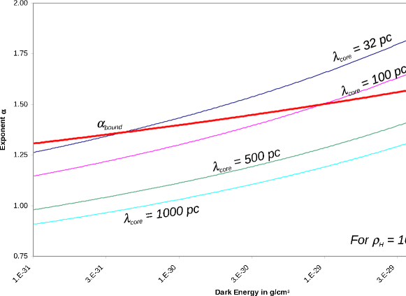
Figure 1: Graphs of ${\alpha_{\Lambda}}$ with respect to $\Lambda_{DE}$ at $\rho_{H}=10^{-24}$ g/cm³ for various values of $\lambda_{\hbox{\scriptsize{core}}}\leq r_{H}$. The graph of the lower experimental bound Eq. $(\ref{alphaBound})$ is also included.

IV The Density Profile of the Model Galaxy

In both Regions I and II, $\rho_{H}\gg\Lambda_{DE}/2\pi$ and Eq. $(\ref{rhoEOM})$ may be approximated as the following,

$$f(\mathbf{{u}})=\rho-\left(\frac{\Lambda_{DE}}{8\pi\rho}\right)^{1+\alpha_{\Lambda}}\left\{\mathbf{\nabla}_{u}^{2}\rho-(1+\alpha_{\Lambda})\frac{|\mathbf{\nabla}_{u}\rho|^{2}}{\rho}\right\},$$ (36)

where ${u}=r/\chi^{1/2}\lambda_{DE}$, and $\mathbf{\nabla}_{u}$ denotes derivative write respect to ${u}$. The solution to Eq. $(\ref{rhoI-II-EOM})$ minimizes the following functional of the density:

$$\mathcal{F}[\rho]=\frac{\Lambda_{DE}c^{2}}{8\pi}\left(\chi^{1/2}\lambda_{DE}\right)^{3}\int d^{3}\mathbf{{u}} \Bigg{\{}\frac{1}{2\alpha_{\Lambda}}\Bigg{|}\mathbf{\nabla}_{u}\left(\frac{\Lambda_{DE}}{8\pi\rho}\right)^{\alpha_{\Lambda}}\Bigg{|}^{2}-\frac{\alpha_{\Lambda}}{\alpha_{\Lambda}-1}\left(\frac{\Lambda_{DE}}{8\pi\rho}\right)^{\alpha_{\Lambda}-1}+$$ (37)

$$\left(\frac{\Lambda_{DE}}{8\pi\rho}\right)^{\alpha_{\Lambda}}\frac{8\pi f({u})}{\Lambda_{DE}}\Bigg{\}},$$

which we view as an effective free energy for the system. Here, we have chosen the scale as $\Lambda_{DE}c^{2}$.

In Region III, on the other hand, the following linearization of Eq. $(\ref{rhoEOM})$ is appropriate,

$$0=\rho-\frac{1}{1+4^{1+{\alpha_{\Lambda}}}}\mathbf{\nabla}^{2}_{u}\rho.$$ (38)

We will find from a detailed analysis of the solution for $\rho$ in Region II that the driving term $f(\mathbf{r})$ is negligibly small in Region III. A calculation of the free energy in this region will not be necessary.

IV.1 The Solution for Region I

For the $v^{\hbox{\scriptsize ideal}}(r)$ curve—corresponding to $\gamma=0$—it is clear that the only solution, $\rho_{I}(r)$, for Eq. $(\ref{rhoI-II-EOM})$ in Region I is the constant solution $\rho_{I}(r)=\rho_{H}$. The free energy for this solution is easily calculated

$${}^{I}\mathcal{F}_{\gamma=0}=-\frac{1}{\alpha_{\Lambda}-1}\frac{\Lambda_{DE}r_{H}^{3}}{6}\left(\frac{\Lambda_{DE}}{8\pi\rho_{H}}\right)^{\alpha_{\Lambda}-1}.$$ (39)

For a general $\gamma>0$, perturbation theory is used to find solutions Eq. $(\ref{rhoI-II-EOM})$. We first scale $\mathfrak{y}=\rho/\rho_{H}$ and $\mathfrak{x}=u/u_{H}\leq 1$, so that

$$\mathfrak{x}^{\gamma}=\mathfrak{y}+\frac{\varepsilon}{\alpha_{\Lambda}}\nabla^{2}\mathfrak{y}^{-\alpha_{\Lambda}},$$ (40)

where the small parameter

$$\varepsilon=\frac{1}{u_{H}^{2}}\left(\frac{\Lambda_{DE}}{8\pi\rho_{H}}\right)^{1+\alpha_{\Lambda}}\sim 10^{-2}\hbox{\textendash}10^{-9},$$ (41)

for $\alpha=3/2$, $\rho_{H}\sim 10^{-24}\hbox{\textendash}10^{-22}$ g/cm³, and $r_{H}\sim 1$ kpc –$\>8$ kpc. There are two approaches to solving Eq. $(\ref{epsilon})$ perturbatively. The first treats the $\nabla^{2}$ term as a perturbation on the solution $\rho_{I}=f$. Doing so gives

$$\rho_{I}^{(a)}(r)=\rho_{H}\left(\frac{r}{r_{H}}\right)^{-\gamma}\left[1-\varepsilon\gamma(1+\gamma\alpha_{\Lambda})\left(\frac{r}{r_{H}}\right)^{\gamma(1+\alpha_{\lambda})-2}\right].$$ (42)

It is valid when $\gamma\geq 2/(1+\alpha_{\lambda})$. For the second, we take $\mathfrak{z}=\varepsilon/\mathfrak{y}^{\alpha}_{\Lambda}$, so that

$$\mathfrak{x}^{-\gamma}=\varepsilon^{1/\alpha_{\Lambda}}\mathfrak{z}^{-1/\alpha_{\Lambda}}+\frac{1}{\alpha_{\Lambda}}\nabla^{2}\mathfrak{z}.$$ (43)

Treating $\varepsilon^{1/\alpha_{\Lambda}}\mathfrak{z}^{-1/\alpha_{\Lambda}}$ now as the perturbation, the solution for $\mathfrak{z}$ that is finite at $\mathfrak{x}=0$ gives

$$\rho_{I}^{(b)}(r) = \left(\frac{\varepsilon(2-\gamma)(3-\gamma)}{\alpha}\right)^{1/\alpha_{\Lambda}}\left(\frac{r}{r_{H}}\right)^{-\widetilde{\gamma}}$$ (44)

$$\left(1+\frac{1}{\alpha}\left[\frac{\varepsilon(2-\gamma)(3-\gamma)}{\alpha}\right]^{1/\alpha_{\Lambda}}\frac{(2-\gamma)(3-\gamma)}{(2-\widetilde{\gamma})(3-\widetilde{\gamma})}\left(\frac{r}{r_{H}}\right)^{2-\widetilde{\gamma}(1+\alpha_{\Lambda})}\right),$$

where $\widetilde{\gamma}=(2-\gamma)/\alpha_{\Lambda}$. The solution is now valid for $\widetilde{\gamma}\leq 2/(1+\alpha_{\Lambda})$, which again corresponds to $\gamma\geq 2/(1+\alpha_{\Lambda})$.

Calculating the free energy for these two perturbative solutions follows straightforwardly. To lowest order in $\varepsilon$, the free energy for $\rho_{I}^{(a)}$ is

$${}^{I}\mathcal{F}_{\gamma>0}^{(a)}=-\frac{1}{\alpha_{\Lambda}-1}\frac{\Lambda_{DE}c^{2}r_{H}^{3}}{6}\left(\frac{\Lambda}{8\pi\rho_{H}}\right)^{\alpha_{\Lambda}-1}\frac{1}{1+\gamma(\alpha_{\Lambda}-1)/3},$$ (45)

while the free energy for $\rho_{I}^{(b)}$ is

$${}^{I}\mathcal{F}_{\gamma>0}^{b}=\frac{\alpha\Lambda c^{2}r_{H}^{3}}{(2-\gamma)(3-\gamma)^{2}}\left(\frac{8\pi\rho_{H}u_{H}}{\Lambda_{DE}}\right)^{2}.$$ (46)

It is clear that ${}^{I}\mathcal{F}_{\gamma=0}<{}^{I}\mathcal{F}^{(a)}_{\gamma\geq 2/(1+\alpha_{\Lambda})}<0<{}^{I}\mathcal{F}^{(b)}_{\widetilde{\gamma}<2/(1+\alpha_{\Lambda})}$. The idealized, pseudoisothermal profile corresponding to $\gamma=0$ is thus the state of lowest free energy in Region I. Physically, this results because of the curvature term $\sim|\nabla\rho|^{2}\geq 0$ in Eq. $(\ref{free-energy})$. Just like the lowest free energy state of a Landau-Ginzberg free energy functional, this term only vanishes for the constant solution; for all other solutions it contributes positively to the free energy.

IV.2 The Solution for Region II

In this region,

$$\frac{1}{3}\rho_{H}\left(\frac{r_{H}}{r}\right)^{\beta}=\rho_{II}-\chi\lambda_{DE}^{2}\left(\frac{\Lambda_{DE}}{8\pi\rho_{II}}\right)^{1+{\alpha_{\Lambda}}}\left\{\mathbf{\nabla}^{2}\rho_{II}-(1+{\alpha_{\Lambda}})\frac{|\mathbf{\nabla}\rho_{II}|^{2}}{\rho_{II}}\right\},$$ (47)

and we denote $\rho_{II}$ as the solution for $\rho$ in Region II. We undertake an asymptotic analysis Bender and Orszag (1978) of Eq. $(\ref{RII-EOM})$ by making the anzatz that within Region II there exists a point $r_{\hbox{\scriptsize{asymp}}}$ beyond which $\rho_{H}(r_{H}/r)^{\beta}/3\ll\rho(r)$. For $r>r_{\hbox{\scriptsize{asymp}}}$, we can then neglect the driving term in Eq. $(\ref{RII-EOM})$, leaving the homogeneous equation

$$0=\rho_{\hbox{\scriptsize{asymp}}}-\left(\frac{\Lambda_{DE}}{8\pi\rho_{\hbox{\scriptsize{asymp}}}}\right)^{1+{\alpha_{\Lambda}}}\left\{\mathbf{\nabla}_{{u}}^{2}\rho_{\hbox{\scriptsize{asymp}}}-(1+{\alpha_{\Lambda}})\frac{|\mathbf{\nabla}_{{u}}\rho_{\hbox{\scriptsize{asymp}}}|^{2}}{\rho_{\hbox{\scriptsize{asymp}}}}\right\}.$$ (48)

IV.2.1 Asymptotic Analysis and the Background Density

We look for a power-law solution to Eq. $(\ref{asympEOM})$ with the form

$$\rho_{\hbox{\scriptsize{asymp}}}=\frac{\Lambda_{DE}}{8\pi}\Sigma({\alpha_{\Lambda}}){u}^{p},$$ (49)

and find that

$$0=-1+\frac{p(1-{\alpha_{\Lambda}}p)}{\bigg{(}\Sigma({\alpha_{\Lambda}})\bigg{)}^{1+{\alpha_{\Lambda}}}}\frac{1}{u^{p(1+{\alpha_{\Lambda}})+2}}.$$ (50)

This gives $p=-2/(1+{\alpha_{\Lambda}})$, with $\Sigma(\alpha_{\Lambda})$ the solution of

$$0=1+\frac{2(1+3{\alpha_{\Lambda}})}{(1+{\alpha_{\Lambda}})^{2}\big{[}\Sigma({\alpha_{\Lambda}})\big{]}^{1+{\alpha_{\Lambda}}}}.$$ (51)

Positivity of $\rho_{\hbox{\scriptsize{asymp}}}$ requires that $\Sigma({\alpha_{\Lambda}})>0$, and this requires that there are positive solutions to Eq. $(\ref{amp})$. Such solutions exist only if ${\alpha_{\Lambda}}$ is the ratio of a odd integer with an even integer. Our choice of ${\alpha_{\Lambda}}=3/2$ satisfies this criteria, and we arrive at the following asymptotic solution

$$\rho_{\hbox{\scriptsize{asymp}}}=\frac{\Lambda_{DE}}{8\pi}\Sigma({\alpha_{\Lambda}})\left(\frac{\chi\lambda_{DE}^{2}}{r^{2}}\right)^{1/(1+{\alpha_{\Lambda}})},$$ (52)

where

$$\Sigma({\alpha_{\Lambda}})=\left[\frac{2(1+3{\alpha_{\Lambda}})}{(1+{\alpha_{\Lambda}})^{2}}\right]^{1/(1+{\alpha_{\Lambda}})}.$$ (53)

To justify our anzatz that $r_{\hbox{\scriptsize{asymp}}}$ lies within Region II, we set $f(r_{\hbox{\scriptsize{asymp}}})=\rho_{\hbox{\scriptsize{asymp}}}(r_{\hbox{\scriptsize{asymp}}})$, and find

$$\frac{r_{\hbox{\scriptsize{asymp}}}}{r_{H}}\leq\left(\frac{8\pi\rho_{H}}{3\Lambda_{DE}}\frac{u_{H}^{2/(1+\alpha_{\Lambda})}}{\Sigma(\alpha_{\Lambda})}\right)^{(1+\alpha_{\Lambda})/2\alpha_{\Lambda}},$$ (54)

where $u_{H}=r_{H}/\chi^{1/2}\lambda_{DE}$. For ${\alpha_{\Lambda}}=3/2$, $\rho_{H}\sim 10^{-24}$ g/cm³, and $r_{H}=1$ kpc, $r_{\hbox{\scriptsize{asymp}}}\leq 1.77r_{H}$; the anzatz is valid through the great majority of Region II for the range of galaxies we are interested in. The upper limit $r_{II}$ to Region II, on the other hand, is found by setting $8\pi\rho_{\hbox{\scriptsize{asymp}}}(r_{II})/\Lambda_{DE}=4$, which gives

$$r_{II}=\left[\frac{1}{4}\Sigma({\alpha_{\Lambda}})\right]^{(1+{\alpha_{\Lambda}})/2}\chi^{1/2}\lambda_{DE}.$$ (55)

For ${\alpha_{\Lambda}}=3/2$, $r_{II}\approx 0.20\>\lambda_{DE}$.

IV.2.2 The Near Core Density

Structural details of the galaxy cannot be seen from $\rho_{\hbox{\scriptsize{asymp}}}$. Instead, we take $\rho_{II}=\rho_{\hbox{\scriptsize{asymp}}}+\rho_{II}^{1}$ and expand Eq. $(\ref{RII-EOM})$ to first order in $\rho_{II}^{1}$,

$$\frac{2(1+3{\alpha_{\Lambda}})}{(1+{\alpha_{\Lambda}})^{2}}\left[\frac{\rho_{H}}{3}\left(\frac{{u}_{H}}{{u}}\right)^{\beta}\right]=\frac{2(1+3{\alpha_{\Lambda}})}{(1+\alpha_{\Lambda})^{2}}\frac{\widehat{\rho}_{II}^{\>1}}{{u}^{2}}+\mathbf{\nabla}^{2}_{u}\widehat{\rho}^{\>1}_{II}.$$ (56)

where $\widehat{\rho}^{\>1}_{II}={u}^{2}\rho^{1}_{II}$. In the special case $\beta=2$, the particular solution to Eq. $(\ref{rho1-EOM})$ is again the constant solution, but now for $\widehat{\rho}^{\>1}_{II}$; this corresponds to $\rho^{1}_{II-\beta=2}=\rho_{H}r_{H}^{2}/3r^{2}$, as expected for an idealized pseudoisothermal profile.

Boundary conditions for $\widehat{\rho}_{II}^{\>1}$ are set at the $r=r_{H}$ surface,

$$\rho_{H}=\rho_{\hbox{\scriptsize{asymp}}}(r_{H})+\frac{\widehat{\rho}_{II}^{\>1}(r_{H})}{{u}_{H}^{2}},\qquad 0=\frac{\partial\rho_{\hbox{\scriptsize{asymp}}}}{\partial{u}}\Bigg{|}_{u_{H}}+\frac{\partial\>\>\>}{\partial{u}}\left(\frac{\widehat{\rho}^{\>1}_{II}}{{u}^{2}}\right)\Bigg{|}_{u_{H}},$$ (57)

where we have made use of the result of the Region I free energy analysis and set $\gamma=0$. The solution to Eq. $(\ref{rho1-EOM})$ for these boundary conditions is

$$\rho_{II}^{1}=\frac{1}{3}A_{\beta}\rho_{H}\left(\frac{r_{H}}{r}\right)^{\beta}+\left(\frac{r_{H}}{r}\right)^{5/2}\left(C_{\cos}\cos\left[\nu_{0}\log\left(\frac{r}{r_{H}}\right)\right]+C_{sin}\sin\left[\nu_{0}\log\left(\frac{r}{r_{H}}\right)\right]\right),$$ (58)

where $\nu_{0}=\left[2(1+3\alpha_{\Lambda})/(1+\alpha_{\Lambda})^{2}-1/4\right]^{1/2}$, and

$$A_{\beta} = \frac{\nu_{0}^{2}+1/4}{\nu_{0}^{2}+(5/2-\beta)^{2}},$$

$$C_{\cos} = \rho_{H}-\frac{1}{3}A_{\beta}\rho_{H}-\frac{\Lambda_{DE}}{8\pi}\frac{\Sigma(\alpha_{\Lambda})}{{{u}_{H}}^{2/(1+\alpha_{\Lambda})}},$$

$$\nu_{0}C_{\sin} = \frac{5}{2}\rho_{H}-\frac{1}{3}A_{\beta}\rho_{H}(5/2-\beta)-\frac{1}{2}\frac{(1+5\alpha_{\Lambda})}{(1+\alpha_{\Lambda})}\frac{\Lambda_{DE}}{8\pi}\frac{\Sigma(\alpha_{\Lambda})}{{{u}_{H}}^{2/(1+\alpha_{\Lambda})}}.$$ (59)

The density $\rho_{II}(r)$ thus consists of the sum of two parts. The first part, $\rho_{\hbox{\scriptsize{asymp}}}(r)$, corresponds to the background density, and depends solely on Dark Energy, fundamental constants, the exponent $\alpha_{\Lambda}$, and the dimensionality and underlying spatial symmetry of the spacetime. It is universal, and has the same form irrespective of the detailed structure of the galaxy. The second part, $\rho_{II}^{1}(r)$, does depend on the detail structure of the galaxy. Variation in $\rho_{II}^{1}$ are measured on a scale set by $r_{H}$, the core size, in contrast to $\rho_{\hbox{\scriptsize{asymp}}}$, whose variations are measured on a scale set by $\lambda_{DE}$, the Dark Energy length scale. While our analysis is done only to first order in the perturbation of $\rho_{II}$, this feature of $\rho_{II}^{1}$ holds to higher orders as well.

The perturbation, $\rho_{II}^{1}$, itself depends on two terms. The first has a power law dependence of $(r_{H}/r)^{\beta}$, while the second has a power law dependence of $(r_{H}/r)^{5/2}$. Thus, near the galactic core $\rho_{II}^{1}\sim r^{-q}$, where $q=\hbox{max}(\beta,5/2)$; to this level of approximation, the density profile near the core varies at least as fast as $1/r^{5/2}$, irrespective of whether the density profile is cuspy or pseudoisothermal. For the $r\gg r_{H}$ the opposite is true, and now $q=\hbox{min}(\beta,5/2)$; $\rho_{II}^{1}$ decreases no faster than $1/r^{5/2}$.

IV.2.3 Free Energy Analysis

The free energy for the density $\rho_{II}$ separates into three terms: ${}^{II}\mathcal{F}={}^{II}\mathcal{F}_{\hbox{\scriptsize{asymp}}}+{}^{II}\mathcal{F}_{\hbox{\scriptsize{asymp}}-\beta}+{}^{II}\mathcal{F}^{1}$, where

$${}^{II}\mathcal{F}_{\hbox{\scriptsize{asymp}}} \equiv \frac{\Lambda_{DE}c^{2}}{8\pi}\left(\chi^{1/2}\lambda_{DE}\right)^{3}\int_{D_{II}}d^{3}\mathbf{{u}}\Bigg{\{}\frac{1}{2\alpha_{\Lambda}}\Bigg{|}\mathbf{\nabla}_{u}\left(\frac{\Lambda_{DE}}{8\pi\rho_{\hbox{\scriptsize{asymp}}}}\right)^{\alpha_{\Lambda}}\Bigg{|}^{2}-$$ (60)

$$\frac{\alpha_{\Lambda}}{\alpha_{\Lambda}-1}\left(\frac{\Lambda_{DE}}{8\pi\rho_{\hbox{\scriptsize{asymp}}}}\right)^{\alpha_{\Lambda}-1}\Bigg{\}},$$

$$= \frac{4\alpha_{\Lambda}^{2}\Lambda_{DE}c^{2}(\chi^{1/2}\lambda_{DE})^{3/2}\left[\Sigma(\alpha_{\Lambda})\right]^{2}}{(\alpha_{\Lambda}^{2}-1)(1+5\alpha_{\Lambda})\left[\Sigma(\alpha_{\Lambda})\right]^{2(1+\alpha_{\Lambda})}}{u}_{II}^{(1+5\alpha_{\Lambda})/(1+\alpha_{\Lambda})},$$

is the contribution to the free energy due to the background density only. The integration is over Region II, and ${u}_{II}=r_{II}/\chi^{1/2}\lambda_{DE}$.

The second term is

$$\frac{{}^{II}\mathcal{F}_{\hbox{\scriptsize{asymp}}-\beta}}{\left(\chi^{1/2}\lambda_{DE}\right)^{3}} \equiv c^{2}\int_{D_{II}}d^{3}\mathbf{{u}}f(u)\left(\frac{\Lambda_{DE}}{8\pi\rho_{\hbox{\scriptsize{asymp}}}}\right)^{\alpha_{\Lambda}}+$$ (61)

$$\frac{8\pi\alpha_{\Lambda}c^{2}}{\Lambda_{DE}[\Sigma(\alpha_{\Lambda})]^{2(1+\alpha_{\Lambda})}}\int_{\partial D_{II}}u^{4}\rho_{II}^{1}(u)\mathbf{\nabla}\rho_{\hbox{\scriptsize{asymp}}}\cdot d\mathbf{S}.$$

$$= \frac{\alpha_{\Lambda}(8\pi)^{2}c^{2}}{\Lambda_{DE}(1+\alpha_{\Lambda})[\Sigma(\alpha_{\Lambda})]^{2(1+\alpha_{\Lambda})}}\left\{u_{H}^{5}\rho_{II}^{1}(u_{H})\rho_{\hbox{\scriptsize{asymp}}}(u_{H})-u_{II}^{5}\rho_{II}^{1}(u_{II})\rho_{\hbox{\scriptsize{asymp}}}(u_{II})\right\}$$

$$-\frac{\Lambda_{DE}c^{2}(1+\alpha_{\Lambda})^{2}}{2(1+3\alpha_{\Lambda})}\left(\frac{4\pi\rho_{H}}{3\Lambda_{DE}}\right)\Sigma(\alpha_{\Lambda})u_{H}^{\beta}\left(\frac{u_{II}^{5-2/(1+\alpha_{\Lambda})-\beta}-u_{H}^{5-2/(1+\alpha_{\Lambda}-\beta)}}{5-2/(1+\alpha_{\Lambda})-\beta}\right),$$

where $\partial D_{II}$ is the boundary of $D_{II}$ at $r=r_{H}$ and $r=r_{II}$. This is the contribution to the free energy due to the interaction between $\rho_{\hbox{\scriptsize asymp}}$ and $f(\mathbf{r})$. It is straightforward to see that

$${}^{II}\mathcal{F}_{\hbox{\scriptsize{asymp}}-\beta}\sim\left\{\begin{array}[]{ll}-(u_{H}/u_{II})^{\beta}&\mbox{if $\beta<5/2$,}\\ -(u_{H}/u_{II})^{5/2}&\mbox{if $5/2\leq\beta<5-2/(1+\alpha_{\Lambda})$.}\\ \pm u_{H}^{5-2/(1+\alpha_{\Lambda})}&\mbox{if $5-2/(1+\alpha_{\Lambda})\leq\beta$,}\end{array}\right.$$ (62)

where the sign of the last term depends on the values of $\beta,\alpha_{\Lambda},u_{H}$ and $\rho_{H}$. The magnitude of this term is very small, however, and it is clear that ${}^{II}\mathcal{F}_{\hbox{\scriptsize{asymp}}-\beta=0}<{}^{II}\mathcal{F}_{\hbox{\scriptsize{asymp}}-\beta<5-2/(1+\alpha_{\Lambda})}<{}^{II}\mathcal{F}_{\hbox{\scriptsize{asymp}}-\beta>5-2/(1+\alpha_{\Lambda})}$.

The third term

$${}^{II}\mathcal{F}^{1} \equiv -\frac{\alpha_{\Lambda}(1+\alpha_{\Lambda})c^{2}\left(\chi^{1/2}\lambda_{DE}\right)^{3}}{2[\Sigma(\alpha_{\Lambda})]^{2(1+\alpha_{\Lambda})}}\int_{\partial D_{II}}u^{4}\rho_{II}^{\>1}(u)\frac{\mathbf{\nabla}\rho_{\hbox{\scriptsize{asymp}}}}{\rho_{\hbox{\scriptsize{asymp}}}}\cdot d\mathbf{S}+\frac{\alpha_{\Lambda}\left(\chi^{1/2}\lambda_{DE}\right)^{3}}{[\Sigma(\alpha_{\Lambda})]^{2(1+\alpha_{\Lambda})}}\left(\frac{8\pi c^{2}}{\Lambda_{DE}}\right)$$ (63)

$$\int_{D_{II}}d^{3}\mathbf{{u}}\Bigg{\{}\frac{1}{2}\left|\mathbf{\nabla}_{u}\widehat{\rho}_{II}^{\>1}\right|^{2}-\frac{(1+3\alpha_{\Lambda})}{(1+\alpha_{\Lambda})^{2}}\frac{(\widehat{\rho}_{II}^{\>1})^{2}}{{u}^{2}}+\frac{2(1+3\alpha_{\Lambda})}{(1+\alpha_{\Lambda})^{2}}f(u)\widehat{\rho}_{II}^{\>1}\Bigg{\}}$$

is the contribution to the free energy due to $\rho_{II}^{1}$ only. As it $\sim(\rho_{II}^{1})^{2}$, this term is very small compared to the other two terms that make up the free energy, and can be neglected. We only note that like ${}^{I}\mathcal{F}$, it is the constant solution to the differential equation that gives the lowest value of ${}^{II}\mathcal{F}^{1}$, but now the equation is for $\widehat{\rho}_{II}^{\>1}=u^{2}\rho_{II}^{1}$, not $\rho_{II}^{1}$. This once again corresponds to $\beta=2$, and as such, to a $\rho_{II}^{1}\sim 1/r^{2}$.

The total free energy, ${}^{II}\mathcal{F}$, in this region is thus smaller for $\beta=2$ than for $\beta>2$. Combined with the calculation for ${}^{I}\mathcal{F}$, we conclude that the pseuodoisothermal rotational velocity curve will result in a density profile that gives the lowest free energy, and is the preferred state of the system. Other rotational velocity curves will result in density profiles that have a higher free energy. We therefore take $\gamma=0$ and $\beta=2$ for the rest of this paper.

IV.3 The Solution for Region III

The solution to Eq. $(\ref{rhoIII-EOM})$ follows using standard methods, with the boundary condition $\rho_{II}(r_{II})=\rho_{III}(r_{II})$. The length scale $\sqrt{\chi/(1+4^{1+{\alpha_{\Lambda}}}})\lambda_{DE}\approx 0.15\>\lambda_{DE}$ for ${\alpha_{\Lambda}}=3/2$, while $r_{II}\approx 0.20\>\lambda_{DE}$; to a good approximation $r_{II}\approx\sqrt{\chi/(1+4^{1+{\alpha_{\Lambda}}})}\lambda_{DE}$. As $\sqrt{\chi/(1+4^{1+{\alpha_{\Lambda}}}})\lambda_{DE}$ is a scale set by the theory, we shall use this last expression for $r_{II}$ from now on. Note also that Regions II and III overlap, and our approach of solving the nonlinear partial differential equation is self-consistent.

The only solution that is spherically symmetric and finite at $r\to\infty$ is

$$\rho_{III}(r)=\frac{\Lambda_{DE}}{8\pi}\Sigma({\alpha_{\Lambda}})\frac{\sqrt{\chi}\lambda_{DE}}{r}\left(1+4^{1+{\alpha_{\Lambda}}}\right)^{\frac{1}{2}(1-{\alpha_{\Lambda}})/(1+{\alpha_{\Lambda}})}\exp\left(1-\frac{r}{\lambda_{DE}}\sqrt{\frac{1+4^{1+{\alpha_{\Lambda}}}}{\chi}}\right),$$ (64)

and in this region the density decreases exponentially fast.

IV.4 The Effective Potential

Note that Eq. $(\ref{NREOM})$ may be written in terms of an effective potential, $\mathfrak{V}(\mathbf{x})$, as $\ddot{\mathbf{x}}=-\mathbf{\nabla}\mathfrak{V}$ where

$$\mathfrak{V}(\mathbf{x})=\Phi(\mathbf{x})+c^{2}\log\mathfrak{R}[4+8\pi\rho/\Lambda_{DE}].$$ (65)

It is thus not the gravitational potential $\Phi(\mathbf{x})$ that determines the dynamics, but $\mathfrak{V}(\mathbf{x})$. To see the implications of this, we begin by calculating $\Phi(\mathbf{x})$, but only for Regions I and II. In Region III, $r>r_{II}$, and motion in this region is unphysical.

Integrating $\mathbf{\nabla}^{2}\Phi=4\pi G\rho$ gives in Region I

$$\Phi(r)=\frac{1}{2}v_{H}^{2}\left(\frac{r}{r_{H}}\right)^{2}-\frac{c^{2}}{2},$$ (66)

where the $c^{2}$ term comes from requiring $\Phi(r_{II})=-c^{2}/2$ instead of $\Phi(\infty)=0$. That this is the usual expression for the Newtonian potential can be seen from $\rho_{H}=3v_{H}^{2}/4\pi Gr_{H}^{2}$. For Region II,

$$\Phi(r)= \frac{c^{2}}{4\alpha_{\Lambda}}\frac{\chi\Sigma(\alpha_{\Lambda})(1+\alpha_{\Lambda})^{2}}{(1+3\alpha_{\Lambda})}{u}^{2\alpha_{\Lambda}/(1+\alpha_{\Lambda})}-2\pi Gr^{2}\rho_{II}^{1}(r)\frac{(1+\alpha_{\Lambda})^{2}}{(1+3\alpha_{\Lambda})}+v_{H}^{2}\log\left(\frac{r}{r_{h}}\right)+$$ (67)

$$-\frac{c^{2}}{2}+v_{H}^{2}\left[1+4\frac{(1+\alpha_{\Lambda})^{2}}{(1+3\alpha_{\Lambda})}\right]-\frac{1}{4}c^{2}\chi\Sigma(\alpha_{\Lambda})\frac{(3+5\alpha_{\Lambda})(1+\alpha_{\Lambda})}{(1+3\alpha_{\Lambda})}u_{H}^{2\alpha_{\Lambda}/(1+\alpha_{\Lambda})}-$$

$$\left\{6v_{H}^{2}\frac{(1+\alpha_{\Lambda})^{2}}{(1+3\alpha_{\Lambda})}-\frac{c^{2}}{2}\chi\Sigma(\alpha_{\Lambda})\frac{(1+\alpha_{\Lambda})(1+2\alpha_{\Lambda})}{(1+3\alpha_{\Lambda})}u_{H}^{2\alpha_{\Lambda}/(1+\alpha_{\Lambda})}\right\}\frac{r_{H}}{r}.$$

The $1/r$ terms in $\Phi$ are expected from Newtonian gravity, and is due to the boundary conditions for $\Phi$ at $r=r_{H}$; this is true for the constant terms as well. The logarithmic term is due specifically to the driving term $f(\mathbf{r})$, as expected. It is a long-range potential that extends out to $r_{II}$, and could potentially explain the non-Newtonian interaction between galaxies and galactic clusters in addition to the galactic rotation curves. The $\rho_{II}^{1}(r)r^{2}$ term is due to the perturbation in the background density, and contains terms $\sim 1/r^{1/2}$. It is due to both the boundary terms in $\rho_{II}^{1}$ and the boundary conditions for $\Phi(r)$. Finally, the $u^{2\alpha_{\Lambda}/(1+\alpha_{\Lambda})}$ term in Eq. $(\ref{potential})$ is due to the background density $\rho_{\hbox{\scriptsize{asymp}}}$, with origins rooted in the rest mass of the test particle. Note also that this term is less than $c^{2}$, verifying that the nonrelativistic limit still holds.

The $c^{2}$ term in $\Phi(r)$ increases as $r^{6/5}$ for $\alpha_{\Lambda}=3/2$, and would dominate the motion of test particles in the galaxy if the extended GEOM depended on $\Phi(\mathbf{x})$ instead of $\mathfrak{V}(\mathbf{x})$. Instead, it and the $r^{2}\rho_{II}^{1}$ term are canceled by the additional density-dependent terms in Eq. $(\ref{effPot})$. To see this, in Regions I and II $\rho>>\Lambda_{DE}/2\pi$, and expanding Eq. $(\ref{effPot})$ gives

$$\mathfrak{V}(\mathbf{x})=\frac{1}{2}v_{H}^{2}\left(\frac{r}{r_{H}}\right)^{2}-\frac{c^{2}}{2}+\frac{c^{2}\chi}{2\alpha_{\Lambda}}\left(\frac{\Lambda_{DE}}{8\pi\rho_{H}}\right)^{\alpha_{\Lambda}},$$ (68)

in Region I, while in Region II,

$$\mathfrak{V}(\mathbf{x})=\Phi(\mathbf{x})-\frac{\chi c^{2}(1+\alpha_{\Lambda})^{2}}{4\alpha_{\Lambda}(1+3\alpha_{\Lambda})}\left(\frac{8\pi u^{2}}{\Lambda_{DE}}\right)\left(\rho_{\hbox{\scriptsize{asymp}}}-\alpha_{\Lambda}\rho^{1}_{II}\right),$$ (69)

where we used $\rho_{II}^{1}/\rho_{\hbox{\scriptsize{asymp}}}<<1$ and Eq. $(\ref{amp})$. The last two terms of Eq. $(\ref{eff-pot})$ cancels the first two terms of Eq. $(\ref{potential})$, and $\mathfrak{V}(r)$ is simply the remaining five terms in Eq. $(\ref{potential})$; the effective potential thus increases only logarithmically as $r$ increases. This is what is expected for a potential that determines the motion of the stars in galactic rotation curves.

That the motion of stars in the galaxy is determined by $\mathfrak{V}(\mathbf{x})$ and not $\Phi(\mathbf{x})$ has far reaching implications. The $c^{2}$ term in $\Phi(\mathbf{r})$ comes from the background density $\rho_{\hbox{\scriptsize{asymp}}}$, and thus the majority of the mass in a stationary galaxy does not contribute to the motion of test particles in the galaxy. Rather, it is the near-core density $\rho_{II}^{1}$ that contributes to $\mathfrak{V}(\mathbf{x})$, which results in the very long-range, logarithmic potential that is observed. As such, observations of the rotational velocity curve of a galaxy will be able to determine the perturbation on the background density, $\rho_{II}^{1}$, but not $\rho_{\hbox{\scriptsize{asymp}}}$ itself. Consequently, since $\rho_{\hbox{\scriptsize{asymp}}}(r)\gg\rho_{II}^{1}(r)$ when $r\gg r_{H}$, the majority of the mass in the universe cannot be seen with these methods. In particular, the motion of stars in galaxies can only be used to estimate $\rho(r)-\rho_{\hbox{\scriptsize{asymp}}}(r)$; the matter in $\rho_{\hbox{\scriptsize{asymp}}}(r)$ is present, but cannot be “seen” in this way.

This behavior is expected for a background density. In the traditional theory of structure formation, the perturbation is off the average density of matter of the universe. This density is usually taken to be a constant, and thus cannot affect the motion of stars within the galaxy. It also fits well with our interpretation that the extension of the GEOM is due to the replacement of the constant rest mass $m$ with a curvature-dependent rest mass. While the rest mass contributes to the Newtonian gravitational potential energy for geodesic motion, it is a constant, and does not contribute to the dynamics of the particle. We see a similar effect here. Our $\rho_{\hbox{\scriptsize asymp}}$ is not a constant, however. It increases as $r\to r_{H}$, and this is a feature expected of cold dark matter. Indeed, we will find below that $R_{200}$ is determined primarily by $\rho_{\hbox{\scriptsize{asymp}}}$. As such, in the absence of all other forces the majority of the mass outside of the galaxy cannot be observed through its dynamics. Other means would have to be used.

V Cosmology

In the previous sections, we have focused on analysing the structure of a single galaxy. In this section, we will extrapolation these results to the cosmological scale, and perform a cosmological check of our theory. That this extrapolation can be done is based on the following two observations

First, recent measurements from WMAP and the Supernova Legacy Survey put $\Omega_{K}=-0.011_{\pm 0.012}$, while WMAP and the HST key project set $\Omega_{K}=-0.014_{\pm 0.017}$ Spergal (2007). In both cases, measurements have shown that the universe is essentially flat, and WMAP’s determination of $h=0.732_{-0.032}^{+0.031}$ was made under this assumption, as is age of the universe $t_{0}$ at $13.73_{-0.15}^{+0.16}$ Gyr. As such, the largest distance between galaxies is $ct_{0}\equiv\mathfrak{K}(\Omega)\lambda_{H}$, where $\mathfrak{K}(\Omega)$ depends on the details of how the universe evolves, and thus on its thermal history; from measurements of both $h$ and $t_{0}$, $\mathfrak{K}(\Omega)=1.03_{\pm 0.05}$.

Second, the density of matter of our model galaxy dies off exponentially fast at $r_{II}$. The extent of the mass of matter in the galaxy is thus fundamentally limited to $2r_{II}$. This size does not depend on the detailed structure of the galaxy near its core; it is inherent to the theory. Moreover, as we can express

$$r_{II}=\left[\frac{8\pi\chi}{3\Omega_{\Lambda}(1+4^{1+\alpha_{\Lambda}})}\right]^{1/2}\lambda_{H}$$ (70)

where $\Omega_{\Lambda}=0.716_{\pm 0.055}$ Spergal (2007) is the fractional density of Dark Energy in the universe, we find that for $\alpha_{\Lambda}=3/2$, $r_{II}=0.52\>\lambda_{H}$. Thus, although the value of $\alpha_{\Lambda}$ was set to $3/2$ by the structure of the galaxy on a galactic scale, the density distribution for the galaxy naturally cuts off at a radius equal to half to Hubble scale, which is precisely what is expected from cosmology.

To accomplish the extrapolation, we use the properties of a representative galaxy for the observed universe to construct our model galaxy. This representative galaxy could, in principal, be found by sectioning the observed universe into three-dimensional, non-overlapping cells centered on a galaxy; given the spatial inhomogeneity of the distribution of galaxies, these cells will not all be the same size. Through a survey of these galactic cells, a representative galaxy, with some average rotational velocity $v_{H}^{*}$ and core radius $r^{*}_{H}$, can be found, and used to set the parameters for our model galaxy. While such a survey has not yet been done, there exists in the literature a large repository of measurements of galactic rotation curves and core radii Blok (2001); Courteau (1997); Mathewson (1992). Taken as a whole, these 1393 galaxies are reasonably random, and are likely representative of the observed universe at large.

While we were able to estimate of $\alpha_{\Lambda}=3/2$ by looking at the galactic structure, the accuracy of this estimate is unknown; comparison with experiment will thus not possible. We instead require that $r_{II}=\mathfrak{K}(\Omega)\lambda_{H}/2$, which gives $\alpha_{\Lambda}$ as the solution of $\mathfrak{K}(\Omega)^{2}(1+4^{1+\alpha_{\Lambda}})=32\pi\chi(\alpha_{\Lambda})/3\Omega_{\Lambda}$; this sets $\alpha_{\Lambda}=1.51_{\pm 0.11}$.

V.1 $\sigma_{8}$, $R_{200}$, and Galactic Rotation Curves

Linear fluctuations in the density are defined as $\delta(\mathbf{r})=\delta\rho/\langle\rho\rangle$ Turner (1990), where $\langle\rho\rangle$ is the spatially-averaged density of matter in a set volume. The rms fluctuation of $\delta$ is measured through $\sigma_{8}^{2}\equiv\langle(\delta(\mathbf{x})^{2}\rangle_{8}$, where the subscript denotes a spatial average over $D_{8}$, a sphere with radius $8h^{-1}$ Mpc. In calculating $\sigma_{8}$, we choose as our origin the center of the unit cell containing the representative galaxy mentioned above. One estimate of the size of a typical unit cell as $5h^{-1}$ Mpc, the characteristic length scale for the galaxy-galaxy correlation function Turner (1990); as this is only slightly smaller the $8h^{-1}$, it is reasonable to consider the density from only a single galaxy within $D_{8}$.

In our theory, $\rho(r)$ varies significantly across $D_{8}$. We thus begin by calculating

$$\langle\rho\rangle_{8} \equiv \langle\rho_{H}\theta(r_{H}-r)\rangle_{8}+\langle\rho_{\hbox{\scriptsize{asymp}}}(r)\theta(r-r_{H})\rangle_{8}+\langle\rho_{II}^{1}(r)\theta(r-r_{H})\rangle_{8},$$ (71)

$$= \frac{3\Lambda_{DE}}{8\pi}\left(\frac{1+\alpha_{\Lambda}}{1+3\alpha_{\Lambda}}\right)\Sigma(\alpha_{\Lambda}){u}_{8}^{-2/(1+\alpha_{\Lambda})}D(u_{8})$$

where $\theta(x)$ is the step function, ${u}_{8}=8h^{-1}\hbox{Mpc}/\chi^{1/2}\lambda_{DE}$, and

$$\zeta=\frac{2{u}_{8}^{-2\alpha_{\Lambda}/(1+\alpha_{\Lambda})}}{\Sigma(\alpha_{\Lambda})\chi(\alpha_{\Lambda})}\left(\frac{v_{H}^{*}}{c}\right)^{2}.$$ (72)

The function

$$D(u_{8}) \equiv 1-y_{8}^{\frac{1+3\alpha_{\Lambda}}{1+\alpha_{\Lambda}}}+\left[\frac{1+3\alpha_{\Lambda}}{1+\alpha_{\Lambda}}\right]\Bigg{\{}\beta+\frac{3y_{8}(1+\alpha_{\Lambda})^{2}}{2(1+3\alpha_{\Lambda})}\left[\nu_{0}\widetilde{C}_{\sin}-\frac{1}{2\nu_{0}}\widetilde{C}_{\cos}\right]-$$

$$\frac{3y_{8}^{\frac{1}{2}}(1+\alpha_{\Lambda})^{2}}{2(1+3\alpha_{\Lambda})}\left(\left[\nu_{0}\widetilde{C}_{\cos}+\frac{1}{2}\widetilde{C}_{\sin}\right]\sin\left[\nu_{0}\log y_{8}\right]+\left[\nu_{0}\widetilde{C}_{\sin}-\frac{1}{2}\widetilde{C}_{\cos}\right]\cos\left[\nu_{0}\log y_{8}\right]\right)\Bigg{\}},$$

where $y_{8}=u_{H}/u_{8}$, and

$$\widetilde{C}_{\cos}\equiv\frac{2}{3}\zeta-\frac{1}{3}y^{2\alpha_{\Lambda}/(1+\alpha_{\Lambda})},\qquad\nu_{0}\widetilde{C}_{\sin}\equiv\frac{7}{3}\zeta-\frac{1}{6}\left(\frac{1+5\alpha_{\Lambda}}{1+\alpha_{\Lambda}}\right)y^{2\alpha_{\Lambda}/(1+\alpha_{\Lambda})}.$$ (74)

Information on the structure of the galaxy is contained in $\zeta$. As $\zeta\sim 5\times 10^{-3}$ for $v_{H}^{*}=200$ km/s, $D(u_{8})\approx 1$, and it is the background density $\rho_{\hbox{\scriptsize{asymp}}}$ that dominates $\langle\rho\rangle_{8}$, and not the detail structure of the galaxy.

This is not the case for $\langle\delta(\mathbf{x})^{2}\rangle_{8}$, which involves the integration of $(\rho_{II})^{2}$ over $D_{8}$. Because $\left(\rho_{II}^{1}\right)^{2}\sim 1/r^{4}$, it is now the behavior of the density near the core that is relevant. Indeed, we find

$$\sigma_{8}^{2}= -1+\frac{1}{3D(u_{8})^{2}}\left(\frac{1+3\alpha_{\Lambda}}{1+\alpha_{\Lambda}}\right)^{2}\Bigg{\{}\frac{1+\alpha_{\Lambda}}{3\alpha_{\Lambda}-1}+2\zeta\left(\frac{1+\alpha_{\Lambda}}{\alpha_{\Lambda}-1}\right)\left(1-y_{8}^{(\alpha_{\Lambda}-1)/(\alpha_{\Lambda}+1)}\right)+$$ (75)

$$\frac{3}{2}(1+\alpha_{\Lambda})\left[\nu_{0}\widetilde{C}_{\sin}-\frac{(\alpha_{\Lambda}-3)}{2(1+\alpha_{\Lambda})}\widetilde{C}_{\cos}\right]y_{8}^{(\alpha_{\Lambda}-1)/(\alpha_{\Lambda}+1)}-$$

$$\frac{3}{2}(1+\alpha_{\Lambda})y_{8}^{1/2}\Bigg{(}\left[\nu_{0}\widetilde{C}_{\cos}+\frac{(\alpha_{\Lambda}-3)}{2(1+\alpha_{\Lambda})}\widetilde{C}_{\sin}\right]\sin[\nu_{0}\log y_{8}]+$$

$$\qquad\qquad\quad\>\>\qquad\left[\nu_{0}\widetilde{C}_{\sin}-\frac{(\alpha_{\Lambda}-3)}{2(1+\alpha_{\Lambda})}\widetilde{C}_{\cos}\right]\cos[\nu_{0}\log y_{8}]\Bigg{)}+$$

$$\frac{4\zeta^{2}}{y_{8}}+\frac{3}{1+(1+3\alpha_{\Lambda})/(1+\alpha_{\Lambda})^{2}}\left(\nu_{0}\widetilde{C}_{\sin}+\frac{3}{2}\widetilde{C}_{\cos}\right)\frac{\zeta}{y_{8}}+$$

$$\frac{9}{4}\left[\widetilde{C}_{\sin}^{2}+\widetilde{C}_{\cos}^{2}+\frac{1}{1+\nu_{0}^{2}}\left(\widetilde{C}_{\sin}^{2}-\widetilde{C}_{\cos}^{2}+2\nu_{0}\widetilde{C}_{\cos}\widetilde{C}_{\sin}\right)\right]\frac{1}{y_{8}}\Bigg{\}},$$

$$\approx \frac{4}{3}\frac{1}{(\alpha_{\Lambda}+1)(3\alpha_{\Lambda}-1)}+\frac{1}{3}\left(\frac{1+3\alpha_{\Lambda}}{1+\alpha_{\Lambda}}\right)^{2}\Bigg{\{}\frac{8\alpha_{\Lambda}\zeta}{(\alpha_{\Lambda}-1)(3\alpha_{\Lambda}-1)}+\frac{\zeta^{2}}{y_{8}}\Bigg{[}5+\frac{81}{4(1+\nu_{0}^{2})}$$ (76)

$$\frac{10}{1+(1+3\alpha_{\Lambda})/(1+\alpha_{\Lambda})^{2}}\Bigg{]}\Bigg{\}},$$

where for Eq. $(\ref{sigma-8})$ we have kept the lowest order terms in $\zeta$ and $y_{8}$. The first term in Eq. $(\ref{sigma-8})$ is due to the background density $\rho_{\hbox{\scriptsize{asymp}}}$. It depends only on $\alpha_{\Lambda}$, and contributes a set amount of 0.141 to $\sigma_{8}^{2}$ irrespective of the structure of the galaxy. The last term is due primarily to the $1/r^{2}$ term in $\rho_{II}^{1}$, and is due to the rotation curves. This term contributes the largest amount to $\sigma_{8}^{2}$, and depends explicitly on details of the structure of the galaxy through $v_{H}^{*}$ and $r_{H}^{*}$.

While there have been a many studies of galactic rotation curves in the literature, our need is for both the rotational velocity and the core radius of galaxies. This requires both a measurement of of the velocity as a function of the distance from the center of the galaxy, and a fit of the data to some model of the velocity curve. To our knowledge, this analysis has been done in four places in the literature . While each of the data sets were obtained with similar physical techniques, there are distinct differences in their selection of galaxies, in the exact experimental techniques used, and in their fits to rotation curves (see Gentile (2004) for a new method of deriving the rotation curves from H1 data). In fact, the Hubble constant used by each are often different from one another, and from the value of 73.2 km/s/Mpc given by WMAP. The reader is referred to the specific papers for details on how these observations were made. Here, we only note the following:

de Blok et. al. Data Set: de Blok and coworkers made detailed measurements of 60 LSB galaxies McGaugh (2001), and fits to $v^{\hbox{\scriptsize{p-iso}}}(r)$ were done for 30 of them Blok (2001). Later, another set of measurements of 26 LSB galaxies were made by de Blok and Bosma deBlok (2002), of which 24 are different from the 30 listed in Blok (2001). Both the data for the 30 original galaxies, and the 24 subsequent galaxies are used here. Although the authors used various models for determining the mass-to-light ratio in their measurements, we will use the data the comes from the minimum disk model, as this was the one model used for all of the galaxies in the set.

While fits to the NFW density profile were made in Blok (2001); deBlok (2002), we are primarily concerned with the fits by the authors to the pseudoisothermal profile velocity curve Eq. $(\ref{iso-curve})$. As de Blok and coworkers were chiefly concern was with the density parameter $\rho_{H}$ for the profile and $R_{C}$, the fits were made with these two parameters. Standard errors for both $\rho_{H}$ and $R_{C}$ were calculated and given. Our concern is with the asymptotic value of $v_{H}$, however, and as this value is given by $\sqrt{4\pi G\rho_{H}r_{C}^{2}}$, we have calculated $v_{H}$ and its standard error from the published values of $\rho_{H}$ and $R_{C}$ in Blok (2001) to determine $v_{H}^{*}$ for this set. The authors used a value of 75 km/s/Mpc for the Hubble constant.

CF Data Set: In Courteau (1997), Courteau presented observations of the velocity curves for over 300 northern Sb-Sc UGC galaxies, and determined $r_{H}$ for each by fitting the curves to three different velocity curves, one of which is similar to the velocity curve for the pseudoisothermal profile used by de Blok and coworkers,

$$v^{\hbox{\scriptsize vcA}}(r)=\frac{2}{\pi}v_{C}\arctan\left(\frac{r}{r_{t}}\right).$$ (77)

Like $v^{\hbox{\scriptsize p-iso}}(r)$, $v^{\hbox{\scriptsize vcA}}(r)$ can be approximated by the idealized velocity curve $v^{\hbox{\scriptsize ideal}}(r)$ used in our analysis. In the limit $r\gg r_{t}$, $v^{\hbox{\scriptsize vcA}}\approx v_{C}$, which sets $v_{c}=v_{H}$. In the limit $r\ll r_{t}$, $v^{\hbox{\scriptsize vcA}}\approx v_{C}(2r/\pi r_{t})$, which sets $r_{t}=2r_{H}/\pi$. Although there are differences between $v^{\hbox{\scriptsize vcA}}(r)$ and $v^{\hbox{\scriptsize p-iso}}(r)$ within the two limits, our analysis here is based on the idealized velocity curve and all that is needed is the relationship between $r_{H}$, and $r_{t}$ or $R_{C}$.

The second fit was to a velocity curve where the steepness of the transition from the hub and the asymptotic velocity curves could be taken into account as well. Because of the work by de Blok and coworkers in Blok (2001), our focus here will be on the velocity curve Eq. $(\ref{vcA})$, and not this curve. The second velocity curve has a limiting form in the $r\to 0$ limit that only agrees with our idealized profile in one special case, and this case does not hold for all the galaxies analyzed by Courteau using this profile.

The third fit was to Persic, Salucci, and Stel’s Universal Rotation Curve (URC) Persic (1996). While the URC asymptotically approaches a constant velocity, at small $r$ the URC has a $r^{0.66}$ behavior, which is different from $v^{\hbox{\scriptsize{ideal}}}$, $v^{\hbox{\scriptsize{p-iso}}}$, and $v^{\hbox{\scriptsize{vcA}}}$, all of which varies linearly in the small $r$ limit. We therefore did not focus on this velocity curve here.

Values for $v_{C}$ and $r_{t}$ for 351 galaxies was obtained through the VizieR service (http://vizier.u-strasbg.fr/viz-bin/VizieR). The great majority of the rotation curves were based on single observations of the galaxy; only 75 of these galaxies were measured multiple times, with the majority of these galaxies observed twice. The data set reposited at VizieR contained these multiple measurements. We have averaged the value of $v_{C}$ and $r_{t}$ for the galaxy where there are multiple measurements of the same galaxy. The standard error in the repeated measurements of a single galaxy can be extremely large; this was recognized in Courteau (1997). A value of 70 km/s/Mpc was used for the Hubble constant by the author.

Mathewson et. al. Data Set: In Mathewson (1992), a survey of the velocity curves of 1355 spiral galaxies in the southern sky was performed. Later, the rotation curves for these observations were derived in Persic (1996) after folding, deprojecting, and smoothing the Mathewson data. Each of these velocity curves are due to a single observation. Courteau performed a fit of Mathewson’s observations to the velocity curve Eq. $(\ref{vcA})$ for 958 of the galaxies in Courteau (1997) using a Hubble constant of $70$ km/s/Mpc. The results of this analysis is reposited in VizieR as well.

Rubin et. al. Data Set: In the early 1980s, Rubin and coworkers Rubin (1980, 1982); Burstein (1982); Rubin (1985) presented a detailed study of the rotation curves of 16 Sa, 23 Sb, and 21 Sc galaxies. This was not a random sampling of Sa, Sb, and Sc galaxies. Rather, these galaxies were deliberately chosen to span a specified range of Sa, Sb, and Sc galaxies, and as stated in Burstein (1982), averaging values of properties of galaxies in this data set would have little meaning. These measurements can contribute to the combined data set of all four measurements, however, which is why we have included them in our analysis. While values for the core radius were not given, measurements of the rotational velocity as a function of the distance to the center of the galaxy were; we are able to fit the data to the same pseudoisothermal rotation curve Eq. $(\ref{iso-curve})$ used by de Blok, et. al. Results of this fit is given in Appendix A.1. A Hubble constant of 50 km/s/Mpc was used by the authors.

Wanting to be as unbiased and as inclusive as possible, we have deliberately not culled through the data sets to select the cleanest of the rotation curves. Nevertheless, we have had to removed the data for 27 galaxies from our analysis. A list of these galaxies and the reason why they were removed are given in Appendix B, where we have listed other peculiarities found with the data sets as well.

The $v_{H}^{*}$ and $r_{H}^{*}$, and standard error for each, were calculated for each of the four data sets considered here. While $v_{H}$ is easily identified for all four, determination of $r_{H}$ is more complicated. For the de Blok et. al. data set, published values of $R_{C}$ was first scaled by $75/73.2$ to account for differences in the Hubble constant used by the authors, and the current value of $73.2$ km/s/Mpc measured by Spergal (2007). Then $r_{H}$ is obtained by using $r_{H}=\sqrt{3}R_{C}$. A similar calculation was made using the calculated values of $R_{C}$ from Appendix A.1, but using $50/73.2$ instead of $75/73.2$ to account for differences in Hubble constants. For the CF and Mathewson et. al. data sets, published values of $r_{t}$ are first scaled by $70/73.2$ to account for differences in Hubble constants, and $r_{H}$ is now obtained using $r_{H}=\pi r_{t}/2$. A fifth data set is then constructed by combining the data from these four data sets. For each data set, $v^{*}_{H}$ and $r^{*}_{H}$ are then used in Eq. $(\ref{full-sig})$ to calculate $\sigma_{8}$; numerical derivatives of $\sigma_{8}$ were then used to calculate its standard error. Not surprisingly, $\Delta\sigma_{8}$ is dominated by the standard error in $\alpha_{\Lambda}$.

Results of these calculations are giving in Table 1, along with the t-test comparison of the calculated $\sigma_{8}$ and $\Delta\sigma_{8}$ with the value $0.761_{-0.048}^{+0.049}$ from Spergal (2007). Surprising, four of the five data sets give a value for $\sigma_{8}$ that is within two-sigma of the WMAP value; they thus agree with the WMAP value at the 95% confidence level. The only data set that differs significantly from the WMAP value is the Rubin et. al. set, and it is known that for this set the selected galaxies are not representative of Sa, Sb. and Sc galaxies; this disagreement is thus not surprising.

Data Set	$v^{*}_{H}$	$\Delta v^{*}_{H}$	$r^{*}_{H}$	$\Delta r^{*}_{H}$	$\qquad\sigma_{8}$	$\qquad\Delta\sigma_{8}$	t-test
deBlok et. al. (53)	119.0	6.8	3.62	0.33	0.613	0.097	1.36
CF (348)	179.1	2.9	7.43	0.35	0.84	0.18	0.43
Mathewson et. al. (935)	169.5	1.9	15.19	0.42	0.625	0.089	1.34
Rubin et. al. (57)	223.3	7.6	1.24	0.14	2.79	0.82	2.46
Combined (1393)	172.1	1.6	11.82	0.30	0.68	0.11	0.70

Table 1: The $v_{H}^{*}$ (km/s), $r_{H}^{*}$ (kps), and resultant $\sigma_{8}$, $\Delta\sigma_{8}$, and t-test comparison with the WMAP value of $\sigma_{8}$. The number of data points in each data set is listed in the parentheses.

While the URC has a different power-law behavior at small $r$ than $v^{\hbox{\scriptsize{ideal}}}$, $v^{\hbox{\scriptsize{p-iso}}}$, or $v^{\hbox{\scriptsize{vcA}}}$, the difference is small enough that it is unknown how $\sigma_{8}$ will change if the URC is used in its calculation instead of the $v^{\hbox{\scriptsize{ideal}}}$ used here. We leave this for future research.

Given $v_{H}^{*}$ and $r_{H}^{*}$, it is possible to calculate $R_{200}$ by setting $u_{8}\to u_{200}=R_{200}/\chi^{1/2}\lambda_{DE}$ in Eq. $(\ref{ave-rho})$, and using $v_{H}^{*}=172.1$ km/s and $r_{H}^{*}=11.82$ kpc from the Combine data set. We numerically solved for this radius and found that $R_{200}=270_{\pm 130}$ kpc, with the large spread coming primarily from the uncertainty in $\alpha_{\Lambda}$.

V.2 Estimating the Fractional Densities of Matter

Because $\rho_{\hbox{\scriptsize{asymp}}}$ is an asymptotic solution and has the same form irrespective the the detail shape of the galaxies, we can estimate $\Omega_{\hbox{\scriptsize asymp}}$ by averaging $\rho_{\hbox{\scriptsize{asymp}}}(r)$ over a sphere of radius $\lambda_{H}/2=r_{II}$,

$$\Omega_{\hbox{\scriptsize{asymp}}}\equiv\frac{\langle\rho_{\hbox{\scriptsize{asymp}}}\rangle_{r_{II}}}{\rho_{c}}\approx\frac{3\Omega_{\Lambda}}{8\pi}\left(\frac{1+\alpha_{\Lambda}}{1+3\alpha_{\Lambda}}\right)\left[2\frac{(1+3\alpha_{\Lambda})}{(1+\alpha_{\Lambda})^{2}}\left(1+4^{1+\alpha_{\Lambda}}\right)\right]^{1/(1+\alpha_{\Lambda})}+\mathcal{O}\left(\frac{r_{H}}{\lambda_{H}}\right)^{3},$$ (78)

where $\rho_{c}$ is the critical density of the universe, and we have used Eq. $(\ref{r-II-Lambda})$. Thus, the ratio $\Omega_{\hbox{\scriptsize asymp}}/\Omega_{\Lambda}$ depends only on the dimensionality and symmetry of spacetime, and the exponent $\alpha_{\Lambda}$. Numerically, we find $\Omega_{\hbox{\scriptsize{asymp}}}=0.197_{\pm 0.017}$.

In performing this average we have implicitly assumed that there is only a single galaxy within the sphere, which is a gross under counting of the number of galaxies in the universe. Note, however, that $\rho_{\hbox{\scriptsize asymp}}(r)$ is an asymptotic solution, and $\rho_{II}^{1}(r)$ is a perturbation off $\rho_{\hbox{\scriptsize asymp}}(r)$ that dies off rapidly with distance. While additional galaxies within the sphere may change the detail form of $\rho_{\hbox{\scriptsize asymp}}$, these changes are expected to be equally short ranged; we thus expect Eq. $(\ref{ratio})$ to be an adequate estimate of $\Omega_{\hbox{\scriptsize asymp}}$.

Such is not the case for $\Omega_{\hbox{\scriptsize{Dyn}}}$. Calculating $\Omega_{\hbox{\scriptsize Dyn}}$ directly by averaging $\rho-\rho_{\hbox{\scriptsize asymp}}$ would require knowing both the detail structure of galaxies, and the distribution of galaxies within the sphere. Instead, we note that $\Omega_{m}=\Omega_{\hbox{\scriptsize asymp}}+\Omega_{\hbox{\scriptsize Dyn}}$, and using the value $\Omega_{m}=0.239_{-0.026}^{+0.025}$ from WMAP, find that $\Omega_{\hbox{\scriptsize{Dyn}}}=0.041^{+0.030}_{-0.031}$. Thus, only a small fraction of the matter in the universe can be seen through their dynamics.

VI Concluding Remarks

Given how sensitive of our expression for $\sigma_{8}$ is dependent on $v_{H}^{*}$, $r_{H}^{*}$, and $\alpha_{\Lambda}$, that our predicted values of $\sigma_{8}$ is within experimental error of its measured value is surprising. This is especially true as the data used in calculating $\sigma_{8}$ was taken by four different groups over a period of 25 years, and for purposes that have no connection whatsoever with our analysis. Even in the absence of a direct experimental search for $\alpha_{\Lambda}$, this provides a compelling argument for the validity of our extension of the GEOM, and its impact on structure formation. This agreement also supports our free energy conjecture; the calculated $\sigma_{8}^{2}$ would be very different if $\beta=3$, say, were used in calculating $\sigma_{8}^{2}$ instead of $\beta=2$.

Direct detection and measurement of $\alpha_{\Lambda}$ through terrestrial experiments may be possible in the near future. As mentioned in Sections II.D and III.B, at a value of $1.51$ the exponent $\alpha_{\Lambda}$ is likely small enough that the effects of the additional terms in the extended GEOM may soon be detectable.

Interestingly, $\Omega_{m}-\Omega_{B}=0.196_{-0.026}^{+0.025}$ is nearly equal to $\Omega_{\hbox{\scriptsize asymp}}$ in value. Correspondingly, $\Omega_{B}$ Spergal (2007) is nearly equal to $\Omega_{\hbox{\scriptsize Dyn}}$. It would be tempting to identify $\Omega_{\hbox{\scriptsize asymp}}$ with the fractional density of nonbaryonic (dark) matter in the universe, especially since matter in $\rho_{\hbox{\scriptsize{asymp}}}(r)$ does not participate in the particle dynamics, and is not “visible” to measurements that inferred mass through particle motion under gravity. That $\Omega_{\hbox{\scriptsize Dyn}}$ would then be identified with $\Omega_{B}$ is consistent with the observation that most of the mass that has been inferred through gravitational dynamics indeed consists of baryons. We did not differentiate between normal and dark matter in our theory, however. Without a specific mechanism for funneling nonbaryonic matter into $\rho_{\hbox{\scriptsize{asymp}}}$ and baryonic matter into $\rho-\rho_{\hbox{\scriptsize{asymp}}}$, we cannot at this point rule out the possibility that $\Omega_{m}-\Omega_{B}=\Omega_{\hbox{\scriptsize{asymp}}}$ and $\Omega_{B}\approx\Omega_{\hbox{\scriptsize Dyn}}$ is a numerical accident.

Appendix A Fits to Data

In Rubin (1985), measurements of the rotational velocity as a function of radius for 60 Sa, Sb and Sc spiral galaxies are given, allowing a fit of this data to $v^{p-iso}(r)$. However, instead of fitting to $v^{\hbox{\scriptsize p-iso}}(r)$ directly as is done in Blok (2001), it is more convenient to fit the data to $(v^{\hbox{\scriptsize p-iso}}(r))^{2}$. As we are interested in the asymptotic velocity $v_{H}$ instead of the density parameter for the pseudoisothermal profile, ours is a two parameter, $(v_{H},R_{C})$, least-squares fit to $(v^{\hbox{\scriptsize p-iso}}(r))^{2}=v_{H}^{2}c(r)$, where

$$c(r)=1-\frac{R_{C}}{r}\arctan\left(\frac{r}{R_{C}}\right).$$ (79)

It uses the variance

$$\sigma_{(v^{\hbox{\scriptsize p-iso}})^{2}}^{2}\equiv\frac{1}{N-2}\sum_{n=1}^{N}[(v^{\hbox{\scriptsize p-iso}}_{n})^{2}-v_{H}^{2}c(r_{n})]^{2},$$ (80)

where $\{(v_{n}^{\hbox{\scriptsize{p-iso}}},r_{n})\}$ is the set of velocity verses radius measurements for a galaxy with a total number of data points $N$. Minimizing with respect to $v_{H}^{2}$ gives

$$v_{H}^{2}=\frac{\langle(v^{\hbox{\scriptsize p-iso}}_{n})^{2}c(r_{n})\rangle}{\langle c(r_{n})^{2}\rangle},$$ (81)

where $\langle\cdots\rangle$ denotes an average over the data points. Minimization with respect to $R_{C}$ gives the implicit equation

$$0=\langle(v^{\hbox{\scriptsize p-iso}}_{n})^{2}c(r_{n})\rangle\left\langle\frac{c(r_{n})r_{n}^{2}}{r_{n}^{2}+R_{C}^{2}}\right\rangle-\langle c(r_{n})^{2}\rangle\left\langle\frac{(v^{\hbox{\scriptsize p-iso}}_{n})^{2}r_{n}^{2}}{r_{n}^{2}+R_{C}^{2}}\right\rangle.$$ (82)

Instead of solving Eq. $(\ref{R-C})$ directly, we substitute Eq. $(\ref{v-infty})$ into Eq. $(\ref{D})$, and find iteratively the $R_{C}$ that minimizes $\sigma^{2}_{(v^{\hbox{\scriptsize p-iso}})^{2}}$. The value for $v_{H}^{2}$ is then found through Eq. $(\ref{v-infty})$.

Standard errors for $v_{H}^{2}$ and $R_{C}$ can be found directly. Taking the implicit derivative of Eq. $(\ref{R-C})$,

$$\frac{\partial R_{C}}{\partial(v^{\hbox{\scriptsize p-iso}}_{i})^{2}}=\frac{R_{C}}{N\Delta}\left\{\frac{\langle c(r_{n})^{2}\rangle r_{i}^{2}}{r_{i}^{2}+R_{C}^{2}}-c(r_{i})\left\langle\frac{c(r_{n})r_{n}^{2}}{r_{n}^{2}+R_{C}^{2}}\right\rangle\right\},$$ (83)

where

$$\Delta\equiv 2\langle(v^{\hbox{\scriptsize p-iso}}_{n})^{2}c(r_{n})\rangle\left\langle\frac{c(r_{n})r_{n}^{4}}{(r_{n}^{2}+R_{C}^{2})^{2}}\right\rangle-2\langle c(r_{n})^{2}\rangle\left\langle\frac{(v^{\hbox{\scriptsize p-iso}}_{n})^{2}r_{n}^{4}}{(r_{n}^{2}+R_{C}^{2})^{2}}\right\rangle+$$ (84)

$$\left\langle\frac{c(r_{n})r_{n}^{2}}{r_{n}^{2}+R_{C}^{2}}\right\rangle\left\langle\frac{(v^{\hbox{\scriptsize p-iso}}_{n})^{2}r_{n}^{2}}{r_{n}^{2}+R_{C}^{2}}\right\rangle-\langle(v^{\hbox{\scriptsize p-iso}}_{n})^{2}c(r_{n})\rangle\left\langle\frac{r_{n}^{4}}{(r_{n}^{2}+R_{C}^{2})^{2}}\right\rangle.$$

The standard error $\sigma_{R_{C}}$ in $R_{C}$ is then

$$\sigma_{R_{C}}=\frac{R_{C}\>\sigma_{(v^{\hbox{\scriptsize p-iso}}_{n})^{2}}\sqrt{\langle c(r_{n})^{2}\rangle}}{\Delta\sqrt{N}}\left\{\langle c(r_{n})^{2}\rangle\left\langle\frac{r_{n}^{4}}{(r_{n}^{2}+R_{C}^{2})^{2}}\right\rangle-\left\langle\frac{c(r_{n})r_{n}^{2}}{r_{n}^{2}+R_{C}^{2}}\right\rangle^{2}\right\}^{1/2}.$$ (85)

For the standard error in $v_{H}^{2}$, we use Eq. $(\ref{v-infty})$ and find

$$\frac{\partial v_{H}^{2}}{\partial(v^{\hbox{\scriptsize p-iso}}_{i})^{2}}=\frac{c(r_{i})}{N\langle c(r_{n})^{2}\rangle}-\left(1+\frac{1}{v_{H}^{2}\langle c(r_{n})^{2}\rangle}\left\langle\frac{v^{\hbox{\scriptsize{p-iso}}}_{n}f_{n}^{2}}{R_{C}^{2}+r_{n}^{2}}\right\rangle-\langle\frac{2}{c(r_{n})^{2}}\rangle\left\langle\frac{c(r_{n})r_{n}^{2}}{R_{c}^{2}+r_{n}^{2}}\right\rangle\right)\frac{v_{H}^{2}}{R_{C}}\frac{\partial R_{C}}{\partial(v^{\hbox{\scriptsize{p-iso}}})^{2}},$$ (86)

resulting in a standard error in $v_{H}$ of

$$\sigma_{v_{H}}=\frac{1}{2}\left[\frac{\sigma^{2}_{(v^{\hbox{\scriptsize p-iso}}_{n})^{2}}}{Nv_{H}^{2}\langle c(r_{n})^{2}\rangle}+\left(1+\frac{1}{v_{H}^{2}\langle c(r_{n})^{2}\rangle}\left\langle\frac{v^{\hbox{\scriptsize{p-iso}}}_{n}r_{n}^{2}}{R_{C}^{2}+r_{n}^{2}}\right\rangle-\frac{2}{\langle c(r_{n})^{2}\rangle}\left\langle\frac{c(r_{n})r_{n}^{2}}{R_{c}^{2}+r_{n}^{2}}\right\rangle\right)^{2}\frac{\sigma_{R_{C}}^{2}}{R_{c}^{2}}\right]^{1/2}.$$ (87)

Our fits of the Rubin et. al. data are tabulated in Table 2. The base data from Rubin (1985) was based on a Hubble constant of $50$ km/s/Mpc, and the results given in Table 2 are for this value of the Hubble constant. Of the 60 galaxies from Rubin (1985), NGC 6314 and IC 724 could not be fitted to a nonzero $R_{C}$, while the fit for NGC 2608 resulted in a $R_{C}$ that is less than $0.01$.

Galaxy	$R_{C}$	$\Delta R_{C}$	$\quad\qquad v_{H}$	$\Delta v_{H}$		Galaxy	$R_{C}$	$\Delta R_{C}$	$\quad\qquad v_{H}$	$\Delta v_{H}$
NGC 1024	0.27	0.14	229.42	9.77		NGC 4800	0.18	0.06	171.56	3.42
NGC 1357	0.52	0.14	268.19	16.27		NGC 7083	0.89	0.14	226.51	2.27
NGC 2639	1.02	0.34	337.69	31.31		NGC 7171	2.25	0.36	251.35	6.47
NGC 2775	0.40	0.17	298.98	8.90		NGC 7217	0.19	0.10	275.21	6.56
NGC 2844	0.41	0.09	167.50	18.93		NGC 7537	0.80	0.10	150.06	2.35
NGC 3281	0.44	0.05	211.32	26.51		NGC 7606	1.40	0.30	279.29	4.11
NGC 3593	0.16	0.08	115.28	14.01		UGC 11810	1.54	0.38	193.28	3.85
NGC 3898	0.53	0.06	254.76	28.73		UGC 12810	3.22	0.35	245.73	1.47
NGC 4378	0.13	0.06	307.61	26.60		NGC 701	2.49	0.58	188.78	4.86
NGC 4419	0.63	0.03	211.55	2.33		NGC 753	0.31	0.11	208.50	3.57
NGC 4594	1.65	0.30	397.24	10.15		NGC 801	0.79	0.16	227.64	4.06
NGC 4698	1.85	0.47	284.96	6.34		NGC 1035	1.24	0.09	150.62	1.26
NGC 4845	0.11	0.07	187.54	0.07		NGC 1087	0.54	0.10	131.91	2.54
UGC 10205	2.19	0.27	272.34	4.07		NGC 1421	0.54	0.13	176.42	3.94
NGC 1085	0.29	0.05	307.02	2.11		NGC 2715	1.10	0.22	151.47	2.93
NGC 1325	1.80	0.28	195.55	2.67		NGC 2742	1.10	0.16	181.86	2.36
NGC 1353	0.36	0.18	218.48	8.30		NGC 2998	1.08	0.22	213.85	3.22
NGC 1417	0.40	0.05	278.87	2.36		NGC 3495	3.11	0.46	206.75	3.22
NGC 1515	0.06	0.10	178.35	10.03		NGC 3672	1.74	0.24	208.11	4.03
NGC 1620	1.73	0.25	241.62	3.14		NGC 4062	0.79	0.13	167.88	2.65
NGC 2590	1.30	0.54	255.24	5.33		NGC 4321	0.79	0.35	208.24	5.42
NGC 2708	1.91	0.68	269.92	9.45		NGC 4605	0.97	0.32	112.62	3.42
NGC 2815	1.91	0.68	269.92	9.45		NGC 4682	1.17	0.23	181.17	2.97
NGC 3054	2.41	0.56	259.10	8.30		NGC 7541	0.21	0.16	195.04	5.94
NGC 3067	0.76	0.06	156.80	1.22		NGC 7664	0.65	0.14	196.05	3.07
NGC 3145	0.15	0.07	257.00	4.84		IC 467	1.64	0.33	152.42	3.26
NGC 3200	0.42	0.09	266.07	5.43		UGC 2885	0.06	0.10	266.22	5.88
NGC 3223	1.35	0.23	275.29	5.51		UGC 3691	3.04	0.33	229.42	1.31
NGC 4448	0.59	0.11	207.02	1.98

Table 2: Fitted values of $R_{C}$ (kpc) and $v_{H}$ (km/s), and their errors for Rubin et. al. data.

Appendix B Data sets

For the de Blok et. al. data set, the galaxy F568-3 was analysed twice; we use analysis of F568-3 given by the authors in Blok (2001). In de Blok and Bosma deBlok (2002), two of the galaxies, F563-1 and U5750, also appeared in Blok (2001); we used the values from Blok (2001) for these galaxies in our analysis. The radius for DDO185 from Blok (2001) was not determined, and we could not include this data point in our analysis. Thus, out of 56 possible galaxies, 53 were used.

For the Rubin et. al. data set, we could not find a nonzero radius for two galaxies, and one galaxy had a radius less than 0.01 kpc. As this radius was smaller than the resolution of their observations, this data point was not included. A total of 57 galaxies were thus used from Rubin (1985).

For the CF and Mathewson et. al. data sets, the vast majority of the data were based on single observations. We therefore had greater leeway in cleaning up this data, but even here we were circumspect. First, 75 galaxies in Courteau (1997) were observed multiple times. Of these, the galaxies UGC 7234 and UGC 10096 had listed an asymptotic velocity for one of the observations that was opposite from the measured asymptotic velocity for the others. We assumed that this was a typographical error, and the sign of the rotational velocity for the anomalous velocity is reversed. Second, five galaxies in the CF and Mathewson et. al. data sets had a $r_{H}=0$, one galaxy had a radius core that was 11-sigma out, and three galaxies had a $v_{H}$ that exceeded 8,000 km/s. These are likely indications that the data was not sufficiently accurate to allow for a fit of the velocity curve, and they were removed. Finally, given that there are only 1393 galaxies combined in the data sets, if a galaxy had a $v_{H}$ or a $r_{H}$ that was six-sigma or more out from the mean, they were removed. In the end, 348 galaxies were used in the CF data set, and 935 galaxies were used in the Mathewson et. al. data set. A summary of the data points not used in our analysis is given in Table 3.

Data Set	Data Removed	Reason	Data Set	Data Removed	Reason
de Blok et. al.	DDO185	$r_{H}=\infty$		ESO 243-G34	$v_{H}$ is 5 $\sigma$ out
Rubin et. al.	NGC 6314	$r_{H}=0$		ESO 317-G41	$r_{H}=0$
	IC 724	$r_{H}=0$		ESO 358-G9	$v_{H}$ is 6 $\sigma$ out
	NGC 2608	$r_{H}<0.01$		ESO 435-G25	$v_{H}$ is 5 $\sigma$ out
CF	UGC 6534	$v_{H}$ is 35 $\sigma$ out		ESO 467-G12	$r_{H}=0$
	UGC 12543	$v_{H}$ is 11 $\sigma$ out		ESO 554-G28	$v_{H}$ is 6 $\sigma$ out
Mathewson et. al.	ESO 140-G28	$v_{H}>8,000$ km/s		ESO 60-G24	$v_{H}$ is 10 $\sigma$ out
	ESO 481-G30	$v_{H}>24,000$ km/s		ESO 359-G6	$r_{H}$ is 11 $\sigma$ out
	ESO 443-G42	$v_{H}>94,000$ km/s		ESO 481-G21	$r_{H}$ is 6 $\sigma$ out
	ESO 108-G19	$r_{H}=0$		UGCA 394	$r_{H}$ is 7 $\sigma$ out
	ESO 141-G34	$r_{H}=0$		ESO 298-G15	$r_{H}$ is 7 $\sigma$ out
	ESO 21-G5	$r_{H}$ is 6 $\sigma$ out		ESO 545-G3	$r_{H}$ is 7 $\sigma$ out
	ESO 548-G21	$r_{H}$ is 7 $\sigma$ out		ESO 404-G18	$r_{H}$ is 9 $\sigma$ out
	NGC 7591	$r_{H}=0$

Table 3: Listed are the galaxies removed from the data sets used in our analysis along with the reason for their removal.