General Connections, Exponential Maps,
and Second-order Differential Equations

Abstract

The main purpose of this article is to introduce a comprehensive, unified theory of the geometry of all connections. We show that one can study a connection via a certain, closely associated second-order differential equation, its geodesic quasispray. One of the most important results is our extended Ambrose-Palais-Singer correspondence. We extend the theory of geodesic sprays to the quasisprays, show that locally diffeomorphic exponential maps can be defined for any SODE, and give a full theory of (possibly nonlinear) covariant derivatives for (possibly nonlinear) connections. In the process, we introduce vertically homogeneous connections. Unlike homogeneous connections, these complete our theory and allow us to include Finsler spaces in a completely consistent manner.

This is an expanded version of the article published in Differ. Geom. Dyn. Syst. 13 (2011) 72–90. Included are the proof published in Nonlinear Anal. 63 (2005) e501–e510 and some new material on homogeneity.

1 Introduction

In modern geometry, there are various kinds of connections for a given manifold $M$ with a bundle structure over it. For example:

• A Cartan connection may be considered as a version of the general concept of a principal connection, in which the geometry of the principal bundle is tied to the geometry of the base manifold [14, 38]. Cartan connections describe the geometry of manifolds modelled on homogeneous spaces. Under certain technical conditions, they can be related to the remaining types [38].

• A general connection on any fibre bundle $E\rightarrow\kern-8.20007pt\rightarrow M$ is a splitting of $TE$ into the natural vertical bundle and a horizontal bundle [25]. If the splitting is equivariant for the structure group (or, more generally, some subgroup) $G$, then it defines an Ehresmann $G$-connection [25, 36].

• A principal connection is an Ehresmann $G$-connection on a principal $G$-bundle $(P,M,G)$ [25, 36].

• A linear connection on a vector bundle $(E,M,V,GL(V))$ over $M$ with model fiber $V$ is associated to a principal connection on the frame bundle with group $GL(V)$ [25, 36]. All others are nonlinear, among which are the affine connections with $G=A_{n}$. It is unfortunate that in the extant literature on nonlinear connections, for example [30, 4, 40, 41, 23] all written well after [25], a nonlinear connection is defined to be a particular highly restricted type of connection on $TM-0$.

• A Koszul connection is a linear operator of the type of a covariant derivative on a vector bundle. It gives rise to a linear connection on the vector bundle [36].

We are only concerned with finite-dimensional real vector bundles $E$ (vector spaces $V$), so $GL(V)\cong GL(n,\mathbb{R})=GL_{n}$ with $n=\dim V$. Moreover, our only direct concern is when $E=TM$, so the principal bundle is $LM$, the bundle of linear frames, $n=\dim M$, and the connections are $G$-connections for a suitable subgroup $G\leq GL_{n}$. All pseudoRiemannian connections are linear connections of this last type [34, 36].

Since the fundamental work of Ehresmann [25], we have had a consistent terminology for connections on a manifold $M$. A connection on $M$ is a splitting $TTM={\mathscr{V}}\oplus\mathscr{H}$ where ${\mathscr{V}}$ is the natural vertical bundle and $\mathscr{H}$ is a complementary subbundle, the horizontal bundle. In this article, we continue our study of smooth general connections on the tangent bundle $TM$ of a smooth, paracompact, connected manifold $M$. We shall use “nonlinear” in the original sense of Ehresmann.

Let us note that Bucataru and Miron [13] recently defined a completely different kind ofnonlinear connection via a generalization of the Koszul procedure. They begin with the assumption that parallel transport is to be linear, construct from that a nonlinear covariant derivative operator, and thence a nonlinear connection. We do not begin with that, or any other such, assumption; instead, we begin with an arbitrary (smooth) nonlinear connection, and then construct a nonlinear covariant derivative operator via an extension of the connector procedure (Def. 4).

The geodesic spray in pseudoRiemannian geometry, the integral curves of which are the geodesics of the Levi-Civita connection, has played an important role; see, for example, [11, 10]. Riemannian geometry has been a main thread of mathematics over the last century [9], and Finsler geometry has recently undergone somewhat of a revival [2].

Second-order differential equations (SODEs) are an important class of vector fields on the tangent bundle. Our principal motivation for this work was the desire to make a comprehensive theory of the geometry of nonlinear connections and SODEs which would include (pseudo)Riemannian geodesic sprays and analogues for Finsler-like spaces as examples. Moreover, such a theory would also apply to the geometry of principal symbols of PDOs [35] and to stability problems around linear connections; e.g., [7, 8].

Section 2 contains our notation, conventions, and a summary of our earlier article [17]. In Section 3 we present the new exponential maps defined by SODEs. Section 4 describes the relations among (possibly nonlinear) connections, certain SODEs (quasisprays), the associated (possibly nonlinear) covariant derivatives, and geodesics. It also contains the various parts of our extended Ambrose-Palais-Singer (APS) correspondence. In Section 5 we provide a simple example using Finsler spaces. Finally, Section 6 begins with the extension of the main results of [8] to SODEs, using our new, extended construction of exponential maps. It also includes the extension of the main stability result of [7, 17] to all SODEs.

The authors thank CONACYT and FAI for travel and support grants, Wichita State University and Universidad Autónoma de San Luis Potosí for hospitality during the progress of this work, and J. Hebda and A. Helfer for helpful conversations. Del Riego also thanks M. Mezzino for writing a Mathematica package for her use.

2 Review and definitions

A second-order differential equation (SODE) on a manifold $M$ is defined as a projectable section of the second-order tangent bundle $TTM\rightarrow\kern-8.20007pt\rightarrow TM$ [11, 10, 12]. Recall that an integral curve of a vector field on $TM$ is the canonical lift of its projection if and only if the vector field is projectable [11]. For a curve $c$ in $M$ with tangent vector field $\dot{c}$, this $\dot{c}$ is the canonical lift of $c$ to $TM$ and $\ddot{c}$ is the canonical lift of $\dot{c}$ to $TTM$. Then each projectable vector field $S$ on $TM$ determines a second-order differential equation on $M$ by $\ddot{c}=S\circ\dot{c}$, and each such curve with $\dot{c}(s_{0})=v_{0}\in T_{c(s_{0})}M$ is a solution with initial condition $v_{0}$. Solutions are preserved under translations of parameter, they exist for all initial conditions by the Cauchy theorem, and, as our manifolds are assumed to be Hausdorff, each solution will be unique provided we take it to have maximal domain; i.e., to be inextendible [11, 16, 29].

There are two vector bundle structures on $TTM$ over $TM$, denoted here by $\pi_{T}$ and $\pi_{*}$. Let $J$ be the canonical involution on $TTM$, so it isomorphically exchanges the two vector bundle structures on $TTM$. We denote the fixed set of $J$ by $\text{fix}\mspace{1.0mu}J$ and observe that it is an affine subbundle of both $\pi_{T}$ and $\pi_{*}$, but not a vector subbundle of either.

• A section $S$ of $TTM$ over $TM$ is a SODE when $JS=S$, or equivalently, when $S\in\Gamma(\text{fix}\mspace{1.0mu}J)$. The space of all SODEs is denoted by $\mathop{\operator@font DE_{2}}\nolimits(M)$, and those vanishing on the 0-section of $TM$ by $\mathop{\operator@font QSpray}\nolimits(M)$.

Thus a SODE can be expressed locally as $S:(x,y)\mapsto(x,y,y,\lower 0.86108pt\hbox{$\mathcal{S}$}(x,y))$.

• If desired, one may work with jet spaces using $J^{1}(\mathbb{R}_{\,0},M)\cong TM$ and $J^{2}(\mathbb{R}_{\,0},M)\cong\text{fix}\mspace{1.0mu}J$, where the notation indicates jets with fixed source $0\in\mathbb{R}$ and target any point in $M$.

The vertical bundle ${\mathscr{V}}=\ker(\pi_{*}:TTM\rightarrow\kern-8.20007pt\rightarrow TM)$ is a vector subbundle with respect to both vector bundle structures on $TTM$. In induced local coordinates, elements of ${\mathscr{V}}$ look like $(x,y,0,Y)$. We observe that $\text{fix}\mspace{1.0mu}J$ is an affine subbundle of $TTM$ with translation vector bundle ${\mathscr{V}}$. This allows us to regard $\mathop{\operator@font DE_{2}}\nolimits(M)$ as an affine space with translation vector space $\Gamma({\mathscr{V}})$ and with $\mathop{\operator@font QSpray}\nolimits(M)$ as a closed affine subspace, so that both are affine nuclear Fréchet spaces [39].

Before commenting further on this definition, we must briefly digress to consider the notion of homogeneity for functions.

Consider the equation $f(ax)=a^{m}f(x)$. In projective geometry, for example, one usually requires this to hold only for $a\neq 0$. We shall call this projectively homogeneous of degree $m$. In other areas, such as Euler’s Theorem in analysis, one further restricts to $a>0$. We shall call this positively homogeneous of degree $m$. Finally, in order that homogeneity of degree 1 coincide with linearity, one must allow all scalars $a\in\mathbb{R}$ (including zero). We shall call this completely homogeneous of degree $m$. By $h(m)$ we shall mean complete homogeneity on $TM$ and projective homogeneity on $TM-0$.

The difference between projective homogeneity and complete homogeneity is minor; essentially, it is just the difference between working on $TM-0$ and on $TM$. The difference between positive homogeneity and the other two is more significant. For example, the inward-going and outward-going radial geodesics of the Finsler-Poincaré plane in [3] have different arclengths.

We must distinguish carefully between parametrized curves and unparametrized paths. A path is the image of a parametrized curve. Alternatively, one may identify paths with equivalence classes of curves: two curves are equivalent if and only if they are reparametrizations of each other. This is clearly a bijective correspondence, as each equivalence class determines a unique path (the common image of all curves in the class) and conversely.

Recall that there are natural vector bundle maps $\mathcal{K}:{\mathscr{V}}\to TM$, respecting $\pi_{T}$, and $\mathcal{J}:\left(\pi^{*}TM\cong TM\oplus TM\right)\to{\mathscr{V}}$ which are isomorphisms on fibers. Both are versions of canonical parallel translation on a vector space. Let $S$ be a SODE over $M$, $p$ a point in $M$, and consider the value $S(0)$ for 0 in $T_{p}M$, a vertical vector in $T_{0}T_{p}M$. Define a vertical vector field by

$$R(u)=\mathcal{J}_{u}\mathcal{K}(S(0))$$ (2.1)

for each $u\in T_{p}M$ and for each $p\in M$. Note that $R$ is vertically constant as it is constant along the fibers of $TM$ in the obvious sense. Clearly, $Q=S-R$ is a quasispray. Moreover, $R$ is the vertical lift $U^{\scriptscriptstyle\mathrm{V}}$ of a vector field $U$ on $M$ as is immediate from the definition [43, p. 6f ]. We may think of $R$ or $U$ as an external force, such as a wind.

We use $\gamma_{u}$ to denote the unique inextendible $S$-geodesic with initial velocity $u\in T_{p}M$, as in [34]. Now we are ready to consider homogeneity for SODEs. Noting that any reasonable notion of homogeneity will force $S$ to be a quasispray and taking into account the decomposition just established, we may as well consider only quasisprays.

• A quasispray $Q$ is homogeneous if and only if for each $0\neq u\in TM$ and all scalars $a\neq 0$, all of the curves $\gamma_{au}$ determine the same unique path in $M$.

Associated with each quasispray is its system of nondegenerate integral curves. A homogeneous qspray gives rise to a system of paths in the sense of Douglas [24], who showed that any such system can be obtained as the paths of the integral curves of a SODE that is $h(2)$. (Note that of all possible $h(m)$, only $h(2)$ is invariantly well-defined globally on $TM$.) We extend our definition of homogenity to systems of paths in the obvious way, so that a system of paths in the sense of Douglas becomes a homogeneous system of paths in our sense.

We are interested primarily in general connections and their derived quasisprays. Thus we are interested in systems of (parametrized) curves so as to include those that arise from inhomogeneous qsprays. It follows that any homogeneous system of paths (a system in the sense of Douglas) is a system of paths in our sense but not conversely; we include inhomogeneous systems while Douglas excluded them.

The following condition is sufficient, but not necessary, for homogeneity as just defined. Denote scalar multiplication in the vertical bundle ${\mathscr{V}}$ by $a_{V}$.

• We say that a SODE $S$ is $h(m)$ when $S(av)=a_{*}a_{V}^{m-1}S(v)$.

Explicitly, $a_{*}a_{V}^{m-1}(x,y,X,Y)=(x,ay,aX,a^{m}Y)$ in induced local coordinates. In other words, the functions $\lower 0.86108pt\hbox{$\mathcal{S}$}(x,y)$ are completely (respectively, projectively) homogeneous of degree $m$ in the vertical component in some induced local coordinates: $\lower 0.86108pt\hbox{$\mathcal{S}$}(x,ay)=a^{m}\lower 0.86108pt\hbox{$\mathcal{S}$}(x,y)$ for some $m\geq 1$ (respectively, $m<1$) and all scalars $a\in\mathbb{R}$ (respectively, $a\neq 0$). Note that $h(m)$ SODEs on $TM$ vanish on the 0-section, so are quasisprays.

The break comes at $m=1$ because an $h(m)$ SODE is to be associated with a connection whose homogeneity formula effectively contains $a^{m-1}$; see Proposition 4.4. In some induced local coordinates, $S:(x,ay)\mapsto(x,ay,ay,a^{m}\lower 0.86108pt\hbox{$\mathcal{S}$}(x,y))$.

• Let $C$ denote the Euler-Liouville vector field on $TTM$. We recall that in local coordinates, $J(x,y,X,Y)=(x,X,y,Y)$ and $C:(x,y)\mapsto(x,y,0,y)$. In the extant literature [17, 27, 28, 31, 32], one finds homogeneous vector fields of degree $m$ defined by $[C,S]=(m-1)S$. In any local coordinates, $S:(x,ay)\mapsto(x,ay,a^{m-1}y,a^{m}\lower 0.86108pt\hbox{$\mathcal{S}$}(x,y))$. It follows that a homogeneous SODE in our theory can be a homogeneous vector field only for $m=2$.

Hereinafter we shall call $h(2)$ SODEs quadratic sprays, in agreement with [28, 31, 32]. (Note that complete homogeneity is required for our quadratic sprays to coincide with the usual spray of [1].) We denote the set of SODEs on $M$ that are $h(m)$ by ${\mathop{\operator@font QSpray}\nolimits}_{m}(M)$. It has been usual to consider only (positive) integral degrees of homogeneity, but we make no such restriction.

Elsewhere [31], projectable vector fields on $TM-0$ are called semisprays and the name sprays (confusingly) used for those that are $h(2)$ on $TM-0$. We will associate a SODE to each (possibly nonlinear) connection in the role of a geodesic spray (see Theorems 4.2 and 4.13), so we shall use the name “quasispray” to reflect this new, extended role (and to distinguish ours from all the others; e.g., [37]). We do, however, explicitly consider only smooth SODEs defined on the entire tangent bundle $TM$; others [2, 3, 31] use only the reduced tangent bundle with the 0-section removed, which is necessary when considering $h(m)$ SODEs when $m<1$ (including $m<0$). In general, one usually requires SODEs to be at least $C^{0}$ across the zero-section when possible; e.g., for Finsler spaces. Most of our results are easily seen to hold mutatis mutandis in these cases as well; any unobvious exceptions will be noted specifically.

As we said, the desire to include Finsler spaces consistently was one of our motivations. What should be the Finsler-geodesic “spray” associated with a Finsler metric tensor is not a homogeneous vector field, but an $h(1)$ SODE in our theory; see [15] for related results. However, the Finsler geodesic coefficients have both $h(2)$ and $h(1)$ parts, making what we shall see in Section 5 is an $h(1)$ semispray.

Several important results concerning quadratic sprays [1, 11, 23, 31] rely on the facts that each such spray $S$ determines a unique torsion-free linear connection $\Gamma$, and conversely, every quadratic spray $S$ arises from a linear connection $\Gamma$ the torsion of which can be assigned arbitrarily. The solution curves of the differential equation $\ddot{c}=S_{\Gamma}\circ\dot{c}$ for a connection-induced spray are precisely the geodesics of that (linear) connection. These solution curves are not only preserved under translations, as is true in general, but also under affine transformations of the parameter $s\mapsto as+b$ for constants $a,b$ with $a\neq 0$. Note that, with our definition, the latter also holds for homogeneous SODEs.

In the general case, a (possibly nonlinear) connection $\Gamma$ gives rise to a quasispray $S$ (see Proposition 4.2), but the correspondence has not been studied before. We shall extend most of the preceding features of the quadratic spray–linear connection correspondence to the general setting. One of our ultimate goals is to determine just how well nonlinear connections can be studied via their quasisprays.

We continue with the principal definitions. Let $S$ be a SODE on $M$.

• We say that a curve $c:(a,b)\rightarrow M$ is a geodesic of $S$ or an $S$-geodesic if and only if the natural lifting $\dot{c}$ of $c$ to $TM$ is an integral curve of $S$.

This means that if $\ddot{c}$ is the natural lifting of $\dot{c}$ to $TTM$, then $\ddot{c}=S(\dot{c})$ is the $S$-geodesic equation.

• We say that $S$ is pseudoconvex if and only if for each compact $K\subseteq M$ there exists a compact $K^{\prime}\subseteq M$ such that each $S$-geodesic segment with both endpoints in $K$ lies entirely within $K^{\prime}$.

If we wish to work directly with the integral curves of $S$, we merely replace “in” and “within” by “over”.

• We say that $S$ is disprisoning if and only if no inextendible $S$-geodesic is contained in (or lies over) a compact set of $M$.

In relativity theory, such inextendible geodesics are said to be imprisoned in compact sets; hence our name for the negation of this property.

Following this definition, we make a convention: all $S$-geodesics are always to be regarded as extended to the maximal parameter intervals (i.e., to be inextendible) unless specifically noted otherwise. When the SODE $S$ is clear from context, we refer simply to geodesics. Note that no SODE can be disprisoning on a compact manifold. However, Corollary 6.2 may be used to obtain results about compact manifolds for which the universal covering is noncompact.

We refer to [17] for motivation, further general results, and results specific to homogeneous SODEs (called homogeneous sprays there), and to [18] for more examples. Note that the SODEs in [17] were positively homogeneous; the extension of those results to complete homogeneity is straightforward, once the definition of homogeneous spray there is corrected to the one for homogeneous SODE here.

3 Exponential maps

Let $S$ be a SODE on $M$. We define the generalized exponential maps (plural!) $\exp^{\varepsilon}$ of $S$ as follows.

First let $p\in M$, $v\in T_{p}M$, and $c$ be the unique $S$-geodesic such that

$$\ddot{c} = S(\dot{c})$$

$$c(0) = p$$

$$\dot{c}(0) = v$$

Define

$$\exp^{\varepsilon}_{p}(v)=c(\varepsilon)$$

for all $v\in T_{p}M$ for which this makes sense. From the existence of flows (e.g., [29, p. 175]), it follows that this is well defined for all $\varepsilon$ in some open interval $(-\varepsilon_{p},\varepsilon_{p})$, which in general depends on $p$, and for all $v$ in some open neighborhood $U_{p}$ of $0\in T_{p}M$, which in general depends on the choice of $\varepsilon\in(-\varepsilon_{p},\varepsilon_{p})$. This defines $\exp^{\varepsilon}_{p}$ at each $p\in M$.

• On $TM-0$, it is frequently convenient to define $\exp^{\varepsilon}_{p}(0)=p$. One must then investigate the regularity near 0 in each case; e.g., in Finsler-related examples it usually turns out to be $C^{1}$.

Next, choose a smooth function $\varepsilon:M\to\mathbb{R}$ such that $\varepsilon(p)\in(-\varepsilon_{p},\varepsilon_{p})$ for every $p\in M$. (The smoothness of $\varepsilon$ is for our later convenience: we want $\exp^{\varepsilon}_{p}$ to be smooth in $\varepsilon$ as well as in all other parameters.) Then the global map $\exp^{\varepsilon}$ is defined pointwise by $(\exp^{\varepsilon})_{p}=\exp^{\varepsilon(p)}_{p}$. The domain of $\exp^{\varepsilon}$ is a tubular neighborhood of the 0-section in $TM$ and the graph of $\varepsilon$ lies in a tubular neighborhood of the 0-section in the trivial line bundle $\mathbb{R}\times M$.

We have an example, given to us by J. Hebda, to show that it is possible that $\varepsilon_{p}<1$ for every open neighborhood of $0\in T_{p}M$ if the SODE is inhomogeneous.

• Consider the SODE on $\mathbb{R}$ given by

  $$\ddot{x}(t)=\pi\left(1+\dot{x}(t)^{2}\right).$$

  To integrate, we rewrite this as

  $$\frac{d\dot{x}}{1+\dot{x}^{2}}=\pi\,dt$$

  and obtain

  $$\arctan\dot{x}=\pi\,t+C_{1}\,.$$

  Thus

  $$\dot{x}(t)=\tan\left(\pi\,t+C_{1}\right),\quad\dot{x}(0)=\tan C_{1}$$

  so

  $$x(t)=\log\bigl{|}\sec\left(\pi\,t+C_{1}\right)\bigr{|}+C_{2}\,.$$

  For $C_{1}\geq 0$, $x$ cannot be continued beyond

  $$\pi t+C_{1} = \frac{\pi}{2}\,,$$

  $$t = \frac{1}{2}-\frac{C_{1}}{\pi}<1\,.$$

  Therefore the usual exponential map of this SODE is not defined (i.e., at $t=\varepsilon=1$) for all $C_{1}\geq 0$.

The closer the graph of $\varepsilon$ gets to the 0-section of $\mathbb{R}\times M$, the larger the tubular neighborhood of the 0-section in $TM$ gets.

Proposition 3.3

For $\varepsilon_{1}<\varepsilon_{2}$, we have $\mathop{\operator@font dom}\nolimits(\exp^{\varepsilon_{\!\!\;1}})\supset\mathop{\operator@font dom}\nolimits(\exp^{\varepsilon_{\!\!\;2}})$, attaining all of $TM$ for $\varepsilon=0$ when $\exp^{0}=\pi$.

This puts the bundle projection $TM\rightarrow\kern-8.20007pt\rightarrow M$ in the interesting position of being a member of a one-parameter family of maps, all of whose other members are local diffeomorphisms. (This is reminiscent of singular perturbations.)

Theorem 3.4

For every $\varepsilon$ such that $0<|\varepsilon|<\varepsilon_{p}$, the generalized exponential map $\exp^{\varepsilon}_{p}$ is a diffeomorphism of an open neighborhood of $0\in T_{p}M$ with an open neighborhood of $p\in M$.

• Proof:  This follows from the flow theorems in ODE (e.g., [29, pp. 175, 302]) and a slight generalization of the usual argument (e.g., [12, p. 116f ]). Note that for $v\in T_{p}M$, $\exp^{\varepsilon}_{p}v=\pi\Phi(\varepsilon,v)$ where $\Phi$ is the local flow of $S$. Then on the 0-section of $TM$, the induced tangent map $(\pi,\exp^{\varepsilon})_{*}$ in block form is given by

  $$\left[\begin{array}[]{cc}0&A\\ I&I\end{array}\right]$$

  where $A$ is invertible. (When $S$ is homogeneous and $\varepsilon=1$, then $A=I$ as in the usual proof.)

If desired, one could use the construction in the proof of Theorem 4.4 in [19] to obtain a more explicit form for this $A$.

For reference, we record the following obvious result.

Lemma 3.5

$\varepsilon$ is a geodesic parameter; i.e., the curve obtained by fixing $v$ and varying $\varepsilon$ is a geodesic through $p$.

Now consider another parameter $a$ as in

$$\exp^{\varepsilon}_{p}(av)\,.$$

In general, $a$ will not be a geodesic parameter; i.e., the curve obtained by fixing $\varepsilon$ and $v$ and varying $a$ is not a geodesic through $p$. See Figures 1 and 2 for a comparison. Also note that these $a$-parameter curves are the exponentials of radial lines in $T_{p}M$.

Figure 1: curves $\exp^{\varepsilon}_{p}(av)$ — Each black curve is a geodesic with $0<\varepsilon<3$ and $a$ and $v$ fixed. From shortest to longest in each plume, $a$ steps in increments of 0.05 from 0.05 to 1. In each plume, $v$ is constant. There are three implicit $a$-parameter curves readily located, one along the endpoints of each of the three plumes.

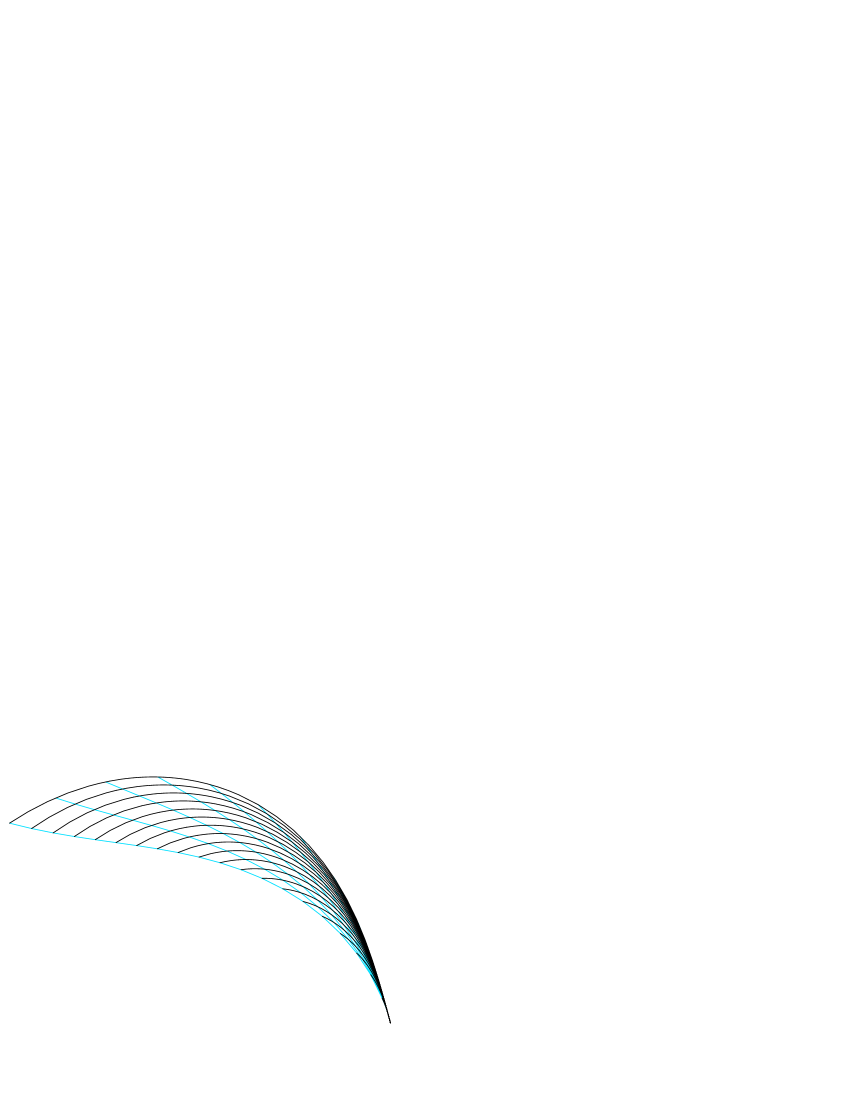
Figure 2: curves $\exp^{\varepsilon}_{p}(av)$ — This is one plume from Figure 1. Each black curve is a geodesic and each gray (blue) curve is an $a$-parameter curve. The new Jacobi fields are along the black curves but tangent to the gray curves.

Proposition 3.6

If $S$ is homogeneous, then $a$ as above is a geodesic parameter.

• Proof:  When $S$ is homogeneous, we can take $\varepsilon=1$ and recover the usual exponential map, and then $a$ is the usual geodesic parameter.

The $a$-parameter curves are interesting: they are the integral curves for our new Jacobi vector fields. These were mentioned in [18] and will be studied in more detail later [20]. For now, we have the following example.

• In $\mathbb{R}^{2}$, consider the SODE given by $\lower 0.86108pt\hbox{$\mathcal{S}$}^{i}(x,y)=y^{i}$ for $i=1,2$. The geodesics are easily found to be $c(t)=ve^{t}+p$ where $v$ is the initial velocity and $p$ is the initial position. We can use the usual exponential map since these curves are always defined for $t=1$. Thus we obtain $\exp_{p}(v)=c(1)=v\,e+p$, regarding both $v$ and $p$ as vectors in $\mathbb{R}^{2}$.

  For the $a$-curves, we have $\exp_{p}(a\,v)=av\,e+p$, showing the difference between the two types quite clearly: the geodesics have exponential growth in velocity, while the $a$-curves have only linear growth.

Finally, note that we could just as well define exponential-like maps based on the $a$-curves and they would share most of the properties of our new exponential maps.

4 Connections and their quasisprays

A (general) connection on a manifold $M$ is a subbundle $\mathscr{H}$ of the second tangent bundle $\pi_{T}:TTM\rightarrow\kern-8.20007pt\rightarrow TM$ which is complementary to the vertical bundle ${\mathscr{V}}$, so

$$TTM=\mathscr{H}\oplus{\mathscr{V}}\,.$$ (4.1)

The space of all connections on $M$ is denoted by $\mathop{\operator@font EConn}\nolimits(M)$, since this definition is essentially due to Ehresmann [25].

Recall there are two vector bundle structures on $TTM$ over $TM$, denoted here by $\pi_{T}$ and $\pi_{*}$. While ${\mathscr{V}}$ is always a subbundle with respect to both [36, pp. 18,20], $\mathscr{H}$ is a subbundle with respect to $\pi_{*}$ if and only if the connection is linear [10, p. 32].

Also recall that quadratic sprays correspond to linear connections. In terms of the horizontal bundle $\mathscr{H}\!,$ linearity is expressed as

$$\mathscr{H}_{av}=a_{*}\mathscr{H}_{v}$$

for $a\in\mathbb{R}$ considered as a map $TM\to TM$ and $v\in TM$. Thus one has

$$\mathscr{H}_{av}=a_{*}a^{m-1}\mathscr{H}_{v}$$ (4.2)

as the second defining equation, together with (4.1), of a connection that is $h(m)$.

• For an $h(m)$ semispray $S$ with integral $m$, Grifone’s [28] associated (generalized) connection coefficients $\Gamma$ are $h(m-1)$, appropriately. See (4.6) below for our version, which allows for inhomogeneous connections.

Here is the SODE induced by a connection. We shall call it the geodesic quasispray associated to the connection and its geodesics the geodesics of the connection.

Theorem 4.2

For each connection $\mathscr{H}\!,$ there is an induced SODE $S$ given by

$$S(v)=\pi_{*}\big{|}^{-1}_{\mathscr{H}_{v}}(v)\,,$$

where $\pi:TM\rightarrow\kern-8.20007pt\rightarrow M$ is the natural projection and $v\in TM$. We write $\mathscr{H}\vdash S$ to denote this relationship.

• Proof:  As in the first paragraph of Poor’s proof of 2.93 [36, p. 95], it is easily verified that $S$ so defined is a SODE. Indeed, $S$ is a section of $\pi_{*}$ by construction, and $S$ is a section of $\pi_{T}$ because $\mathscr{H}$ is a subbundle with respect to $\pi_{T}$.

It is clear that this $S$ is horizontal, so compatible with the given connection, and that it vanishes on the 0-section of $TM$. This latter means that constant curves, $c(t)=p\in M$ for all $t$, are degenerate $S$-geodesics, a familiar property of geodesic sprays. Accordingly, we shall refer to any SODE which vanishes on the 0-section of $TM$ as a quasispray.

Unfortunately, when the connection is $h(m-1)$ this SODE is not homogeneous as a SODE; it is only an $h(m)$ vector field on $TM$. In order to avoid this problem, we must consider a new type of partial homogeneity for connections.

• A connection $\mathscr{H}$ on $TM$ is vertically homogeneous of degree $m$, denoted by $vh(m)$, if and only if

  $$\mathscr{H}_{av}=a_{*}a_{V}^{m-1}\mathscr{H}_{v}$$ (4.3)

  where $a_{V}$ denotes scalar multiplication by $a$ in the vertical bundle ${\mathscr{V}}$.

Note that $h(m)$ and $vh(m)$ coincide only for $m=1$, the linear connections.

Proposition 4.4

If $\mathscr{H}$ is a connection with geodesic quasispray $S$, then $S$ is $h(m)$ if and only if $\mathscr{H}$ is $vh(m-1)$.

• Proof:  That $S$ is $h(m)$ if $\mathscr{H}$ is $vh(m-1)$ follows as in the second paragraph of Poor’s proof of 2.93 [36, p. 95], mutatis mutandis; the converse results from a similar calculation.

Connections may also be seen as sections of the bundle $G_{H}(TTM)$ of all possible horizontal spaces, a subbundle of the Grassmannian bundle $G_{n}(TTM)$. To see what structure $G_{H}(TTM)$ has, consider $\mathbb{R}^{2n}=\mathbb{R}^{n}\oplus\mathbb{R}^{n}$ as the model fiber of $TTM$ and regard the first summand as horizontal, the second as vertical. With $GL_{2n}$ as the structure group of $TTM$, we want the subgroup $A_{H}$ that preserves the vertical space and maps any one horizontal space into another. This can be conceived as occurring in two steps. First, we may apply any automorphisms of the vertical and horizontal spaces separately. Second, we may add vertical components to horizontal vectors to obtain the new horizontal space.

$$\left[\begin{array}[]{cc}I&0\\ \mathfrak{gl}_{n}&I\end{array}\right]\cdot\left[\begin{array}[]{cc}GL_{n}&0\\ 0&GL_{n}\end{array}\right]$$

Our group $A_{H}$ is thus found to be a semidirect product entirely analogous to an affine group. The action is transitive and the right-hand factor is the isotropy group of a fixed horizontal space, so the model fiber for $G_{H}(TTM)$ is the resulting homogeneous space. The induced operation on representatives being given by

$$\left[\begin{array}[]{cc}I&0\\ A&I\end{array}\right]\cdot\left[\begin{array}[]{cc}I&0\\ B&I\end{array}\right]=\left[\begin{array}[]{cc}I&0\\ A+B&I\end{array}\right],$$

it follows that $G_{H}(TTM)$ is an affine bundle (bundle of affine spaces, vs. vector spaces). Thus a connection, being a section of this bundle, provides a choice of distinguished point in each fiber, hence a vector bundle structure on this affine bundle.

If we wish to consider only those connections compatible with a given quasispray, we just replace arbitrary elements of $\mathfrak{gl}_{n}$ with those having a first column comprised entirely of zeros. Note that this yields an affine subbundle $G_{H}^{S}(TTM)$ of $G_{H}(TTM)$, with fibers being pencils of possible horizontal spaces.

Theorem 4.5 (extended APS)

Given a quasispray $S$ on $M$, there exists a compatible connection $\mathscr{H}$ in $TTM$.

Since the fibers of $G_{H}^{S}(TTM)$ are contractible, this is an easy exercise in obstruction theory [22, Ch. 8]; however, an explicit construction is desirable to provide a concrete representation for our extension of the Ambrose-Palais-Singer correspondence, and we gave a detailed proof in [19]. For the convenience of the reader, we repeat the complete proof. First, we provide a brief sketch. It mostly follows the usual outline [36, proof of Thm. 2.98, pp. 97ff ], but (as noted earlier) the exponential maps do not map radial lines in the tangent space into geodesics in the base, so considerable extra care is required to use correct pre-images of geodesics instead.

• Proof:  Let $\Phi$ denote the local flow of $S$ and $\gamma$ an integral curve of $S$ with $\gamma(0)=v\in T_{p}M$. The basic idea is to use $S$ and $\Phi$ to define notions of horizontal and parallel which will coincide with the usual ones along $\gamma$ for any $\mathscr{H}\vdash S$. This is essentially the same as the usual construction [36]. The problem is that for inhomogeneous $S$, the ray $\{tv\}$ in $T_{p}M$ does not exponentiate to a geodesic in $M$.

  To remedy this, we proceed as follows. For each $v\in T_{p}M$, choose $\varepsilon_{v}$ so that $\exp_{p}^{\varepsilon_{\!\!\>v}}v$ is defined. Such $\varepsilon_{v}$ exist by Proposition 3.3. For $0\leq t\leq\varepsilon_{v}$, define

  $$\alpha_{v}(t)=\left(\exp_{p}^{\varepsilon_{\!\!\>v}}\right)^{-1}\exp_{p}^{t}v\,.$$ (4.4)

  Then $\alpha_{v}(0)=0$, $\alpha_{v}(\varepsilon_{v})=v\in T_{p}M$, and $\alpha_{v}$ exponentiates to the geodesic with initial condition $v$ at $p$. Note that if $S$ is homogeneous, then $\alpha_{v}(t)=tv$.

  We have a vector bundle map $\mathcal{J}:\pi^{*}TM\to{\mathscr{V}}$ which is an isomorphism on fibers. It is one version of canonical parallel translation on a vector space, identifying the tangent space at each point with the vector space itself. Now, for each $w\in T_{p}M$ define

  $$\mathscr{H}_{w}=\left\{\left.\frac{d}{dt}\right|_{t=0}\pi_{*}\Phi_{t*}\,\mathcal{J}_{\alpha_{\!\!\;v}(t)}w\Bigm{|}v\in T_{p}M\right\}.$$ (4.5)

  Clearly, this does not depend on the choices of $\varepsilon_{v}$ made earlier. (Note we are evaluating at 0.) If $S$ is quadratic, it is easy to check that this coincides with the usual construction as found in [36, pp. 96–97], since in that case $\exp_{p}tv=\pi\Phi(t,v)$ for $v\in T_{p}M$. The proof that $\mathscr{H}$ so defined is a connection and that $\mathscr{H}\vdash S$ follows Poor’s proof of 2.98 [36, pp. 97–99] mutatis mutandis.

These connections will be our “standard”—our generalization of torsion-free linear connections; viz. equation (4.9), Definition 4 and after. In light of this, and the fact that when applied to pseudoRiemannian geodesic sprays this construction yields the Levi-Civita connection, we shall call them LC connections; cf. Poor [36, 2.104 and 3.29].

• Note that the space of connections $\mathop{\operator@font EConn}\nolimits(M)$ fibers trivially over the space of quasisprays $\mathop{\operator@font QSpray}\nolimits(M)$ since the latter has a vector space structure, albeit not one compatible with that of all vector fields on $TM$.

• Recall that any SODE on $TM-0$ is called a semispray. This is justified by the fact that any construction such as ours that produces a compatible connection over $TM$ from a quasispray there also produces one over $TM-0$ from every SODE there. In particular, this means that for a SODE on $TM$ that is not a quasispray, the restriction of this SODE to $TM-0$ is a semispray with a compatible connection over $TM-0$ even though the original SODE did not have one over $TM$. Such SODEs do not seem to have been noted before, and further study of them is clearly warranted.

Here is an alternative, axiomatic characterization of a connection in terms of the horizontal projection $H$.

• $H$ is a smooth section of $\mathop{\operator@font End}\nolimits(TTM)$ over $TM$.

• $H^{2}=H$.

• $\ker H={\mathscr{V}}$.

Then $\mathscr{H}=\mathop{\operator@font im}\nolimits H$ is the horizontal bundle. Vertical homogeneity is expressed with an optional axiom.

• $H$ is $vh(m)$ if and only if $H_{av}a_{*}=a_{*}a_{V}^{m-1}H_{v}$ for all $v\in TM$ and $a\in\mathbb{R}$ ($v\in TM-0$ and $a\neq 0$ for $m<0$).

Homogeneous connections may be similarly axiomatized.

There is a natural vector bundle map $K:{\mathscr{V}}\to TM$ respecting $\pi_{T}$ which is an isomorphism on fibers, a version of canonical parallel translation of a vector space. Using this, we define a connection map or connector for an arbitrary connection and thence a covariant derivative.

• For a connection $\mathscr{H}\!,$ define the associated connector $\kappa:TTM\to TM:z\mapsto K(z-H_{v}z)$ for $z\in T_{v}TM$.

Proposition 4.9

The connector $\kappa$ is a vector bundle map respecting $\pi_{T}$ but not $\pi_{*}$ in general. It respects $\pi_{*}$ if and only if the connection is linear.

• Proof:  As in Poor [36, p. 72f ], mutatis mutandis.

According to Besse [10, p. 32f ], a symmetric connector (connection) is invariant under the natural involution $J$ of $TTM$. Clearly this is possible only for linear connections.

Now we are ready for the main event. Let $V$ and $U$ be a vector fields on $M$ with $V_{p}=v$ and $U_{p}=u$.

• The covariant derivative associated to the connection $\mathscr{H}$ is the operator defined by

  $$\nabla_{\!U}V=\kappa(V_{*}U)=K(V_{*}U-H_{V}V_{*}U)$$

  and is tensorial in $U$ but nonlinear (in general) in $V$.

This last comes from the general lack of respect for the $\pi_{*}$ structure by $\mathscr{H}\!,$ $H\!$, and $\kappa$.

• We always have $\nabla_{\!0}V=0$. For all $vh(m)$ connections, $\nabla_{\!U}aV=K(a_{*}V_{*}U-H_{aV}a_{*}V_{*}U)=aK(V_{*}U-a_{V}^{m-1}H_{V}V_{*}U)$, and similarly for homogeneous ones. So (vertically) homogeneous connections do not differ significantly from linear ones. In particular, $\nabla_{\!U}0=0$ for all $U$ for all (vertically) homogeneous connections; in fact, they all have the same horizontal spaces along the 0-section of $TM$, namely the subspaces tangent to it (i.e., those in the image of $0_{*}:TM\to TTM$). We call all such connections sharing this property 0-preserving; they differ minimally from (vertically) homogeneous (including linear) connections. In contrast, connections with $\nabla_{\!U}0\neq 0$ for even some $U$ are much farther from linear; we call them strongly nonlinear. See Figure 3 for a schematic view.

Figure 3: Each set of connections is closed with empty interior in the next: linear in homogeneous, linear in vertically homogeneous, linear and homogeneous in 0-preserving, linear and vertically homogeneous in 0-preserving, linear and homogeneous and vertically homogeneous in 0-preserving, 0-preserving in the whole. The strongly nonlinear connections may be visualized as a 3-d cloud containing the 0-preserving ones.

As usual, $\mathfrak{X}$ denotes the vector fields on $M$. There is also a natural vector bundle map $\mathcal{J}:\pi^{*}TM\to{\mathscr{V}}$ which is an isomorphism on fibers, another version of canonical parallel translation on a vector space.

Theorem 4.12

There is a bijective correspondence between (possibly nonlinear) connections $\mathscr{H}$ and our (possibly nonlinear) covariant derivatives $\nabla$ on $TM$.

• Proof:  It suffices to show that we can reconstruct $\mathscr{H}$ from its associated covariant derivative $\nabla$. For each $u\in T_{p}M$, define

  $$\accentset{\hrulefill}{\mathscr{H}}_{u}=\{U_{*}v-\mathcal{J}_{u}\nabla_{\!v}U\mid U\in\mathfrak{X},U_{p}=u,v\in T_{p}M\}$$

  and form the subbundle $\accentset{\hrulefill}{\mathscr{H}}$ in $TTM$ in the obvious way. It is easy to see that $\accentset{\hrulefill}{\mathscr{H}}$ is complementary to ${\mathscr{V}}$ as required, hence a connection. That $\accentset{\hrulefill}{\mathscr{H}}$ is smooth is straightforward. Finally, $\accentset{\hrulefill}{\mathscr{H}}=\mathscr{H}$ from this construction and the construction of $\nabla$ from $\mathscr{H}\!$ [19].

Compare [36, p. 77, proof of 2.58]. Thus as usual, we may refer indifferently to $\mathscr{H}$ or its associated $\nabla$ as the connection.

Generalized connection coefficients may be introduced through

$$\left(KH_{V}V_{*}U\right)^{k}=\Gamma^{k}_{i}(V)U^{i}\,,$$ (4.6)

making manifest the tensoriality in $U$. Here is an example of their use. Observe that $(KV_{*}U)^{k}=U^{i}\partial_{i}V^{k}$ so that

$$\left(\nabla_{\!U}V\right)^{k}=U^{i}\partial_{i}V^{k}-\Gamma^{k}_{i}(V)U^{i}$$ (4.7)

is the covariant derivative.

We find the usual relation between the two notions of geodesic.

Theorem 4.13

A curve $c$ is a geodesic of $\mathscr{H}$ if and only if $\nabla_{\!\dot{c}}\,\dot{c}=0$.

• Proof:  $\nabla_{\!\dot{c}}\,\dot{c}=\kappa(\dot{c}_{*}\dot{c})=K(\dot{c}_{*}\dot{c}-H_{\dot{c}}\,\dot{c}_{*}\dot{c})=K(\dot{c}_{*}\dot{c}-S(\dot{c}))$ by the construction of $S$ in Theorem 4.2. Now all we have to do is identify $\dot{c}_{*}\dot{c}$ as $\ddot{c}$ and recall that $K$ is an isomorphism on fibers.

If we are given the geodesic equation of $\mathscr{H}$ in the form

$$\ddot{c}^{\,k}=\Gamma^{k}_{i}(\dot{c})\dot{c}^{i},$$ (4.8)

then

$$\lower 0.86108pt\hbox{$\mathcal{S}$}^{k}(\dot{c})=\Gamma^{k}_{i}(\dot{c})\dot{c}^{i}$$ (4.9)

gives the quasispray $S$ induced by the connection $\mathscr{H}$. Using these connection coefficients, we obtain the LC connection associated to $S$ by our extended APS construction; see also Theorem 4.17.

Curvature is readily handled. Let $\mathscr{H}$ be a connection on $M$. The horizontal lift of a vector field $U$ on $M$ is defined as usual and denoted by $\bar{U}$.

• Given vector fields $U$ and $V$ on $M$, the curvature operator $R(U,V):TM\to TM$ is defined by

  $$R(U,V)w=\kappa\left([\bar{V},\bar{U}]_{w}\right)$$

  for all $w\in TM$. It is tensorial in the first two arguments, but nonlinear (in general) in the third.

The arguments are reversed on the right in order to obtain the usual formula in terms of the associated covariant derivative,

$$R(U,V)W=\nabla_{\!U}\nabla_{\!V}W-\nabla_{\!V}\nabla_{\!U}W-\nabla_{\![U,V]}W\,,$$

as one may verify readily. It is also easy to check that this curvature vanishes if and only if $\mathscr{H}$ is integrable, thus justifying our definition.

Torsion is considerably more obscure. Consider two (possibly nonlinear) connections $\accentset{\hrulefill}{\mathscr{H}}$ and $\mathscr{H}$ on $TM$ with corresponding (possibly nonlinear) covariant derivatives $\accentset{\hrulefill}{\nabla}$ and $\nabla$.

• Given two covariant derivatives $\accentset{\hrulefill}{\nabla}$ and $\nabla$, define the difference operator $\mathcal{D}=\accentset{\hrulefill}{\nabla}-\nabla$.

We think of $\mathcal{D}$ as having two arguments, $\mathcal{D}(U,V)={\accentset{\hrulefill}{\nabla}}_{\!U}V-\nabla_{\!U}V$. It is always tensorial in $U$, but is nonlinear (in general) in $V$.

We define the covariant differential as usual via $(\nabla V)U=\nabla_{\!U}V$. As an operator, $\nabla V$ is still linear in its argument $U$.

Lemma 4.16

For all $v\in TM$, $\accentset{\hrulefill}{\mathscr{H}}_{v}=\{z-\mathcal{J}_{v}\mathcal{D}(\pi_{*}z,v)\mid z\in\mathscr{H}_{v}\}$.

• Proof:  Let $v\in T_{p}M$, $z\in\mathscr{H}_{v}$, $V\in\mathfrak{X}$ such that $(\nabla V)_{p}=0$ and $V_{p}=v$. Thus if $u=\pi_{*}z\in T_{p}M$, then $z=V_{*}u\in\mathscr{H}_{v}$. Now

  $$\bar{\kappa}V_{*}u={\accentset{\hrulefill}{\nabla}}_{\!u}V=\nabla_{\!u}V+\mathcal{D}(u,V)=\mathcal{D}(u,V)=\bar{\kappa}\mathcal{J}_{v}\mathcal{D}(u,V)\,,$$

  so $\bar{\kappa}\left(z-\mathcal{J}_{v}\mathcal{D}(u,v)\right)=0$ and $z-\mathcal{J}_{v}\mathcal{D}(u,v)\in\accentset{\hrulefill}{\mathscr{H}}_{v}$.

  Since $\pi_{*}$ is an isomorphism of the horizontal spaces $\accentset{\hrulefill}{\mathscr{H}}_{v}$ and $\mathscr{H}_{v}$ with $T_{p}M$ and $\pi_{*}z=\pi_{*}\left(z-\mathcal{J}_{v}\mathcal{D}(u,v)\right)$, this yields all of $\accentset{\hrulefill}{\mathscr{H}}_{v}$.

Compare this next result with [36, Prop. on p. 99].

Theorem 4.17

Two connections on $TM$ have the same geodesic quasispray if and only if their associated difference operator is alternating (vanishes on the diagonal of $TM\oplus TM$).

• Proof:  For each $v\in TM$, $S_{v}=\pi_{*}\big{|}^{-1}_{\mathscr{H}_{v}}(v)$ while $\accentset{\hrulefill}{S}_{v}=\pi_{*}\big{|}^{-1}_{\accentset{\hrulefill}{\mathscr{H}}_{v}}(v)=\pi_{*}\big{|}^{-1}_{\mathscr{H}_{v}}(v)-\mathcal{J}_{v}\mathcal{D}(v,v)$. Therefore $\accentset{\hrulefill}{S}=S$ if and only if $\mathcal{D}(v,v)=0$ for all $v\in TM$.

For linear connections, $\mathcal{D}$ is bilinear and alternating is equivalent to antisymmetric (or, skewsymmetric). In general, of course, this does not hold.

The familiar formula for torsion $T(U,V)=\nabla_{\!U}V-\nabla_{\!V}U-[U,V]$ is not linear (let alone tensorial) in either argument. Thus the usual trick to get a torsion-free linear connection, replacing $\nabla$ by $\accentset{\hrulefill}{\nabla}=\nabla-\mbox{$\textstyle\frac{1}{2}$}T$, will not work for our nonlinear connections. Indeed, $\accentset{\hrulefill}{\nabla}$ and $\nabla$ seem to have the same geodesics and $\accentset{\hrulefill}{\nabla}$ is formally torsion-free, but the new $\accentset{\hrulefill}{\nabla}$ is not one of our nonlinear covariant derivatives: ${\accentset{\hrulefill}{\nabla}}_{\!U}V$ is not tensorial in $U$.

A replacement $\mathcal{T}$ for torsion must also be alternating in order for it to play the same role in general that torsion does for linear connections. For then, given such a $\mathcal{T}$, $\accentset{\hrulefill}{\nabla}=\nabla+\mathcal{T}$ is another nonlinear covariant derivative of our type with the same geodesics as $\nabla$; or, with the same geodesic qspray as $\nabla$.

What we shall do is one of the classic mathematical gambits: turn a theorem into a definition.

• We define the LC connections constructed in the proof of Theorem 4.5 to be the torsion-free connections.

Equivalently, we are regarding the usual torsion formula as derived from the difference operator (difference tensor in the linear case) construction [36, pp. 99–100]. See also Poor [36, pp. 101–102] for the relation to the classic Ambrose-Palais-Singer correspondence and compare to [36, 2.104].

Now we may construct the torsion of a (possibly nonlinear) connection $\mathscr{H}$ with corresponding (possibly nonlinear) covariant derivative $\nabla$. By Theorem 4.2, $\mathscr{H}$ induces a (unique) quasispray $S$. Use the proof of Theorem 4.5 to construct the connection $\hat{\mathscr{H}}$ from $S$. By Theorem 4.12 there is a unique covariant derivative $\hat{\nabla}$ corresponding to $\hat{\mathscr{H}}$. Let $\mathcal{D}=\nabla-\hat{\nabla}$ be the difference operator, so $\hat{\nabla}=\nabla-\mathcal{D}$ is torsion-free.

• Using the preceding notations, the (generalized) torsion of $\nabla$ is defined by $\mathcal{T}=2\mathcal{D}=2\left(\nabla-\hat{\nabla}\right)$.

The factor of two here and the subtraction order make verification that this reduces to classical torsion in the linear case immediate, and preserves the traditional formula $\hat{\nabla}=\nabla-\mbox{$\textstyle\frac{1}{2}$}\mathcal{T}$ for the associated torsion-free connection. See Poor [36, 2.105] for how this fits into the classical APS correspondence.

5 Finsler spaces

For the benefit of those readers not familiar with Finsler geometry, we offer a few introductory and historical remarks.

Finsler spaces are manifolds whose tangent spaces carry a norm (rather than an inner product; cf. Banach vs. Hilbert spaces) that varies smoothly with the base point. Although Riemann actually defined such spaces in his 1854 Habilitationsvortrag, the modern name comes from P. Finsler’s thesis of 1918 in which he studied the variational problem in regular metric spaces.

Geometric objects on a Finsler space depend not only on the base point but also on the fiber component. Classically, a Finsler metric is given by a fundamental function $F$ which is continuous on $TM$, smooth and positive on $TM-0$, and positively homogeneous of degree one in the fiber component. An orthogonal structure on the vertical bundle is defined by the vertical Hessian of the square of the fundamental function. A differentiable manifold $M$ with a Finsler metric is called a Finsler space. One modern variation is to consider only a subset of $TM$ as the domain of $F$, with appropriate changes to the rest of the definition.

We define the Finsler functions $L$, the basic function, and the traditional $F$, the fundamental function, following two of the seemingly overlooked but prescient papers of Beem [5, 6].

We require $L$ to be $h(2)$ and note that it corresponds to $F^{2}$, but to get pseudoRiemannian structures we must require only that $L$ be real valued, not strictly positive, else we could not have spacelike, timelike, and null geodesics, as first observed by Beem [5]. We also require that $L$ be continuous on $TM$ and smooth on $TM-0$, following tradition.

Then we use $|L|^{\frac{1}{2}}$ as the correspondent to $F$; e.g., in the first variation formula (viz. [34, Chapt. 10]) to obtain non-null geodesics. We shall see later how to obtain the null geodesics.

The vertical Hessian

$$g_{ij}(y)=\frac{1}{2}\frac{\partial^{2}}{\partial y^{i}\partial y^{j}}L(y)$$ (5.1)

is traditionally assumed positive definite, which perforce yields only Riemannian entities, such as the traditional orthogonal structure on the vertical bundle ${\mathscr{V}}(TM-0)$. We shall merely assume it is nondegenerate, allowing pseudoRiemannian entities. Together with our relaxed condition on $L$, this gives us pseudoFinsler (or indefinite Finsler) structures as first defined by Beem around 1969 [5].

The traditional geodesic coefficient is [3]

$$G^{i}(y)=\frac{1}{2}g^{il}(y)\left[\frac{\partial}{\partial x^{k}\partial y^{l}}L(y)y^{k}-\frac{\partial}{\partial x^{l}}L(y)\right].$$

To be consistent with our conventions, we take the negative of this for our geodesic coefficients,

$$\mathcal{G}^{i}(x,y)=-G^{i}(x,y)$$ (5.2)

where we have restored the explicit $x$ and $y$ dependence. These components $\mathcal{G}^{i}$ then make up a semispray function $\mathcal{G}$ with accompanying $h(1)$ geodesic semispray $G$. In induced local coordinates,

$$G:(x,y)\mapsto(x,y,y,\mathcal{G}(x,y))\,.$$

The traditional Finsler geodesic equations are

$$\ddot{c}^{i}+G^{i}(\dot{c})=0\,.$$

In our notation and conventions, this becomes

$$\ddot{c}=G(\dot{c})\,.$$ (5.3)

The traditional nonlinear connection coefficients are

$$N^{i}_{j}=\frac{\partial}{\partial y^{j}}G^{i}.$$

Converting to our notation and formalism, we obtain the $vh(0)$ nonlinear connection on $TM-0$ given locally by

$$\Gamma^{i}_{j}(x,y)=\frac{\partial}{\partial y^{j}}\mathcal{G}^{i}(x,y)\,.$$ (5.4)

In fact, this last equation holds in complete generality, as can be seen easily from (4.9). We chose to take note of it here in recognition of the historical context.

Once we have the (nonlinear) connection $\mathscr{H}$ determined by $\Gamma$, we obtain the associated (nonlinear) covariant derivative $\nabla$ from Definition 4; it is unique by Theorem 4.12. Using this connection, we may then recoup (Theorem 4.13) all the (timelike and spacelike) geodesics found in Finsler geometry tradition via the First Variation, and we also obtain all the null geodesics, which cannot [34, Chapt. 10] be so found. Therefore, as first noted by Beem [6], we do indeed have genuine pseudoFinsler geometry.

6 Geodesic connectivity and stability

In [17], we defined a SODE to be LD if and only if its usual exponential map is a local diffeomorphism. For some results there, we used the fact that the geodesics of such SODEs give normal starlike neighborhoods of each point in $M$. (In fact, the $a$-curves also give such neighborhoods, as is easily seen.) Thanks to our new exponential maps (Section 3), these results now immediately extend to all SODEs. For convenience, we state them here.

Proposition 6.1

Let $M$ be a manifold with a pseudoconvex and disprisoning SODE $S$. If $S$ has no conjugate points, then $M$ is geodesically connected.

Let $M$ be a manifold with a SODE $S$ and let $\widetilde{M}$ be a covering manifold. If $\phi:\widetilde{M}\rightarrow M$ is the covering map, then it is a local diffeomorphism. Thus $\tilde{S}=(\phi_{\ast})^{\ast}S$ is the unique SODE on $\widetilde{M}$ which covers $S$, geodesics of $\tilde{S}$ project to geodesics of $S$, and geodesics of $S$ lift to geodesics of $\tilde{S}$. Also, $S$ has no conjugate points if and only if $\tilde{S}$ has none. The fundamental group is simpler, and $\tilde{S}$ may be both pseudoconvex and disprisoning even if $S$ is neither.

Corollary 6.2

Let $M$ be a manifold with a pseudoconvex and disprisoning SODE $S$ and let $\widetilde{M}$ be a covering manifold with covering SODE $\tilde{S}$. If $\tilde{S}$ has no conjugate points, then both $\widetilde{M}$ and $M$ are geodesically connected.

Theorem 6.3

Let $S$ be a pseudoconvex and disprisoning SODE on $M$. If $S$ has no conjugate points, then for each $p\in M$ the exponential maps of $S$ at $p$ are diffeomorphisms.

We remark that none of these results require (geodesic) completeness of the SODE $S$.

We now consider the joint stability of pseudoconvexity and disprisonment for SODEs in the fine topology. Because each linear connection determines a (quadratic) spray, Examples 2.1 and 2.2 of [7] show that neither condition is separately stable. (Although [7] is written in terms of principal symbols of pseudodifferential operators, the cited examples are actually metric tensors). We shall obtain $C^{0}$-fine stability, rather than $C^{1}$-fine stability as in [7], due to our effective shift from potentials to fields as the basic objects. The proof requires some modifications of that in [7]; we shall concentrate on the changes here and refer to [7] for an outline and additional details.

Rather than considering $r$-jets of functions, we now take $r$-jets of sections in defining the Whitney or $C^{r}$-fine topology as in Section 2 of [7]. Let $h$ be an auxiliary complete Riemannian metric on $M$. Thus we look at the $C^{r}$-fine topology on the sections of $TTM$ over $TM$.

If $\gamma_{1}$ and $\gamma_{2}$ are two integral curves of a SODE $S$ with $\gamma_{1}(0)=(x,v)$ and $\gamma_{2}(0)=(x,\lambda v)$ for some positive constant $\lambda$, then the inextendible geodesics $\pi\circ\gamma_{1}$ and $\pi\circ\gamma_{2}$ no longer differ only by a reparametrization. Thus, in contrast to [7], we must now consider an integral curve for each non-zero tangent vector at each point of $M$. Note this also means that we can no longer use the $h$-unit sphere bundle to obtain compact sets in $TM$ covering compact sets in $M$.

Observe that the equations of geodesics involve no derivatives of $S$. Thus if $\gamma:[0,a]\rightarrow TM$ is a fixed integral curve of $S$ in $TM$ with $\gamma(0)=v_{0}\in TM$ and if $\gamma^{\prime}:[0,a]\rightarrow TM$ is an integral curve of $S^{\prime}$ in $TM$ with $\gamma^{\prime}(0)=v$, then $d_{h}\left(\pi\circ\gamma(t),\pi\circ\gamma^{\prime}(t)\right)<1$ for $0\leq t\leq a$ provided that $v$ is sufficiently close to $v_{0}$ and $S^{\prime}$ is sufficiently close to $S$ in the $C^{0}$-fine topology. This and the $\sigma$-compactness of $TK_{1}$ when $K_{1}$ is compact yield the following result.

Lemma 6.4

Assume $K_{1}$ is a compact set contained in the interior of the compact set $K_{2}$, $V$ is an open neighborhood of $K_{2}$, $S$ is a disprisoning SODE, and let $\epsilon>0$. There exist countable sets $\{v_{i}\}\subseteq TK_{1}$ of tangent vectors and $\{\delta_{i}\}$ and $\{a_{i}\}$ of positive constants such that if $S^{\prime}$ is in a $C^{0}$-fine $\epsilon$-neighborhood of $S$ over $V$, then the following hold:

1. if $c$ is an inextendible $S$-geodesic with $c(0)$ in a $\delta_{i}$-neighborhood of $v_{i}$, then $c[0,a_{i}]\subset V$ and $c(a_{i})\in V-K_{2}$;

2. If $c^{\prime}$ is an inextendible $S^{\prime}$-geodesic with $\dot{c}^{\prime}(0)$ in a $\delta_{i}$-neighborhood if $v_{i}$, then $c^{\prime}[0,a_{i}]\subset V$ and $c^{\prime}(a_{i})\in V-K_{2}$;

3. Two inextendible geodesics, $c$ of $S$ and $c^{\prime}$ of $S^{\prime}$ with $\dot{c}(0)$ and $\dot{c}^{\prime}(0)$ in a $\delta_{i}$-neighborhood of $v_{i}$, remain uniformly close together for $0\leq t\leq a_{i}$;

4. The union of all the $\delta_{i}$-neighborhoods of the $v_{i}$ covers $TK_{1}$.

Continuing to follow [7], we construct the increasing sequence of compact sets $\{A_{n}\}$ which exhausts $M$ and the monotonically nonincreasing sequence of positive constants $\{\epsilon_{n}\}$. The only additional changes from [7, p. 17f ] are to use integral curves of $S$ in $TM$ instead of bicharacteristic strips in $T^{*}M$. No other additional changes are required for the proof of the next result either.

Lemma 6.5

Let $S$ be a pseudoconvex and disprisoning SODE and let $S^{\prime}$ be $\delta$-near to $S$ on $M$. If $c^{\prime}:(a,b)\rightarrow M$ is an inextendible $S^{\prime}$-geodesic, then there do not exist values $a<t_{1}<t_{2}<t_{3}<b$ with $c^{\prime}(t_{1})\in A_{n}$, $c^{\prime}(t_{3})\in A_{n}$, and $c^{\prime}(t_{2})\in A_{n+4}-A_{n+3}$.

Now we establish the stability of pseudoconvex and disprisoning SODEs by showing that the set of all SODEs in $\mathop{\operator@font DE_{2}}\nolimits(M)$ which are pseudoconvex and disprisoning is an open set in the $C^{0}$-fine topology. The only changes needed from the proof of Theorem 3.3 in [7, p. 19] are replacing principal symbols by SODEs, bicharacteristic strips by integral curves, $S^{*}A_{n}$ by $TA_{n}$, and references to Lemma 3.2 there by references to Lemma 6.5 here.

Theorem 6.6

If $S\in\mathop{\operator@font DE_{2}}\nolimits(M)$ is pseudoconvex and disprisoning, then there is some $C^{0}$-fine neighborhood $W(S)$ in $\mathop{\operator@font DE_{2}}\nolimits(M)$ such that each $S^{\prime}\in W(S)$ is both pseudoconvex and disprisoning.

Corollary 6.7

If $M$ is a pseudoconvex and disprisoning pseudoRiemannian manifold, then all (possibly nonlinear) connections on $M$ which are sufficiently close to the Levi-Civita connection are also pseudoconvex and disprisoning.

References

- [1] W. Ambrose, R. S. Palais and I. M. Singer, Sprays, Anais Acad. Brasil Ciênc. 32 (1960) 163–178.
- [2] P. L. Antonelli, ed. Handbook of Finsler Geometry. Dordrecht: Kluwer, 2003.
- [3] D. Bao, S.-S. Chern, and Z. Shen, An Introduction to Riemann-Finsler Geometry. New York: Springer, 2000.
- [4] W. Barthel, Nichtlineare Zusammenhänge und deren Holonomiegruppen, J. reine angew. Math. 212 (1963) 120–149.
- [5] J. K. Beem, Indefinite Finsler spaces and timelike spaces, Can. J. Math 22 (1970) 1035–1039.
- [6] J. K. Beem, On the indicatrix and isotropy group in Finsler spaces with Lorentz signature, Atti Accad. Naz. Lincei Rend. Cl. Sci. Fis. Mat. Natur. 54 (1973), 385–392 (1974).
- [7] J. K. Beem and P. E. Parker, Whitney stability of solvability, Pac. J. Math. 116 (1985) 11–23.
- [8] J. K. Beem and P. E. Parker, Pseudoconvexity and geodesic connectedness, Ann. Mat. Pura Appl. 155 (1989) 137–142.
- [9] M. Berger, A Panoramic View of Riemannian Geometry. Berlin: Springer-Verlag, 2003.
- [10] A. L. Besse, Manifolds all of Whose Geodesics are Closed. New York: Springer-Verlag, 1978.
- [11] F. Brickell and R. S. Clark, Differentiable Manifolds. New York: Van Nostrand, 1970.
- [12] Th. Bröcker and K. Jänich, Introduction to Differential Topology. Cambridge: U. P., 1982.
- [13] I. Bucataru and R. Miron, Finsler-Lagrange Geometry: Applications to dynamical systems. Bucharest: Ed. Academiei Romane, 2007.
- [14] E. Cartan, L’extension du calcul tensoriel aux géométries non-affines, Ann. Math. 38 (1937) 1–13.
- [15] L. Del Riego, 1-homogeneous sprays in Finsler manifolds, in Global Differential Geometry: The Mathematical Legacy of Alfred Gray, eds. Marisa Fernández and Joseph A. Wolf. Contemp. Math. 288. Providence: AMS, 2001. pp. 411–414.
- [16] L. Del Riego and C. T. J. Dodson, Sprays, universality and stability, Math. Proc. Camb. Phil. Soc. 103 (1988) 515–534.
- [17] L. Del Riego and P. E. Parker, Pseudoconvex and disprisoning homogeneous sprays, Geom. Dedicata 55 (1995) 211–220.
- [18] L. Del Riego and P. E. Parker, Some nonlinear planar sprays, in Nonlinear Analysis in Geometry and Topology, ed. T. M. Rassias. Palm Harbor: Hadronic Press, 2000. pp. 21–52.
- [19] L. Del Riego and P. E. Parker, Geometry of nonlinear connections, Nonlinear Anal. 63 (2005) e501–e510.
- [20] L. Del Riego and P. E. Parker, Jacobi Fields, Automorphisms, and Holonomy of Connections, in preparation.
- [21] L. Del Riego and P. E. Parker, Automorphism and Holonomy Groups of Ehresmann Connections, in preparation.
- [22] C. T. J. Dodson and P. E. Parker, A User’s Guide to Algebraic Topology. Boston: Kluwer Academic Publishers, 1997.
- [23] P. Dombrowski, On the geometry of the tangent bundle, J. reine angew. Math. 210 (1962) 73–88.
- [24] J. Douglas, The general geometry of paths, Ann. Math. 29 (1927–1928) 143–168.
- [25] C. Ehresmann, Les connexions infinitésimales dans un espace fibré différentiable, in Colloque de topologie (espaces fibrés), Bruxelles, 1950. Paris: Masson et Cie., 1951. pp. 29–55.
- [26] K. Freeman, History of Connections, masters’ thesis, Wichita State University, 2010.
- [27] J. Grifone, Connexions non linéaires conservatives, C. R. Acad. Sci. Paris Sér. A Math. 268 (1969) 43–45.
- [28] J. Grifone, Structure Presque Tangent et Connexions non Homogènes. Thèse cycle, Université de Grenoble, 1971.
- [29] M. W. Hirsch and S. Smale, Differential Equations, Dynamical Systems, and Linear Algebra. New York: Academic Press, 1974.
- [30] A. Kawaguchi, On the theory of non-linear connections I. Introduction to the theory of general non-linear connections, Tensor 2 (1952) 123–142.
- [31] J. Klein and A. Voutier, Formes extérieures géneratrices de sprays, Ann. Inst. Fourier 18 (1968) 241–260.
- [32] M. de León and P. Rodríguez, Methods of Differential Geometry in Analytical Mechanics. Amsterdam: North-Holland, 1989.
- [33] P. Michor, Manifolds of Differentiable Mappings. Orpington: Shiva, 1980.
- [34] B. O’Neill, Semi-Riemannian Geometry. PAM 103. New York: Academic Press, 1983.
- [35] P. E. Parker, Geometry of bicharacteristics, in Advances in Differential Geometry and General Relativity, eds. S. Dostoglou and P. Ehrlich. Contemp. Math. 359. Providence: AMS, 2004. pp. 31–40.
- [36] W. A. Poor, Differential Geometric Structures. New York: McGraw-Hill, 1981. (Dover reprint, 2007.)
- [37] H. Reckziegel, Generalized sprays and the theorem of Ambrose-Palais-Singer, in Geometry and Topology of Submanifolds V, ed. F. Dillen, L. Vrancken, L. Verstraelen, and I. Van de Woestijne. River Edge: World Scientific, 1993. pp. 242–248.
- [38] R. W. Sharpe, Differential Geometry: Cartan’s Generalization of Klein’s Erlangen Program. GTM 166. New York: Springer, 2000.
- [39] F. Trèves, Topological Vector Spaces, Distributions, and Kernels. New York: Academic Press, 1967.
- [40] J. Vilms, Curvature of nonlinear connections, Proc. Amer. Math. Soc. 19 (1968) 1125–1129.
- [41] J. Vilms, Nonlinear and direction connections, Proc. Amer. Math. Soc. 28 (1971) 567–572.
- [42] A. Vondra, Sprays and homogeneous connections on , Arch. Math. (Brno) 28 (1992) 163–173.
- [43] K. Yano and S. Ishihara, Tangent and Cotangent Bundles: Differential Geometry. PAM 16. New York: Marcel Dekker, 1973.