Effective multifractal features and $\ell$-variability diagrams of high-frequency price fluctuations time series

Abstract

In this manuscript we present a comprehensive study on the multifractal properties of high-frequency price fluctuations and instantaneous volatility of the equities that compose Dow Jones Industrial Average. The analysis consists about quantification of dependence and non-Gaussianity on the multifractal character of financial quantities. Our results point out an equivalent influence of dependence and non-Gaussianity on the multifractality of time series. Moreover, we analyse $\ell$-diagrams of price fluctuations. In the latter case, we show that the fractal dimension of these maps is basically independent of the lag between price fluctuations that we assume.

I Introduction

Scale invariance and fractality, i.e., the absence of a characteristic scale can be found in a widespread of natural and human creation phenomena mandelbrot . Mathematically, scale invariance of a certain function, $f$, of an observale $\mathcal{O}$ is written as,

$$f\left(\lambda\mathcal{O}\right)=\lambda^{\alpha}f\left(\mathcal{O}\right),$$ (1)

and it has consensually been considered as a signature of complexity complex . Specifically, power-law behaviour respecting Eq. (1) has empirically been verified in the probability density and autocorrelation functions of several time series such as: fluctuation in heart rate beating peng-heart , gait gait , variation in the magnetic field of the solar wind in the heliosheath nasa , or relative stock price fluctuations bouchaud mantegna among many others. Concerning time series and fractality , if many of them seem to be monofractal feder , i.e., they are characterised by a single scale exponent, just as in Eq.(1), other time series, namely those we have referred to here above, have shown a spectrum of locally dependent $\alpha$ exponents. Analytically, this is noted as

$$f\left(\left\{\lambda\mathcal{O}\right\}^{\upsilon}\right)=\lambda^{\alpha\left(\upsilon\right)}f\left(\mathcal{O}^{\upsilon}\right).$$ (2)

The previous Eq. (2) is also valid for multiscaling and multifractality as well, which has consistently been associated with the main statistical features of time series obtained from complex systems. Consequently, this close relation has been prominent in either the development of dynamical models or validation of previous approaches. In the former case, pioneering works by B. Mandelbrot have opened the door to a new treatment of financial markets dynamics mandelbrot-scaling .

In sequel of this manuscript we perform an extensive analysis of the statistical features of high-frequency price fluctuations, $r_{t}$, of the $30$ equities that compose the Dow Jones Industrial Average (DJIA). Previous studies on daily price fluctuations have shown the existence of a multifractal behaviour djia-daily . Hence, with this high-frequency analysis, it is our aim to study the multiscaling of price fluctuations at a level that is closer to the transaction dynamics as it has been made for other financial observables. Our study is driven on the evaluation of the multifractal spectra of both of time series and $\left(\ell=1\right)$-diagrams, $\left(r_{t},r_{t+1}\right)$, describing their main factors of multifractality. In addition, we enquire into price fluctuations absolute values, $\left|r_{t}\right|$, also called as instantaneous volatility, $v_{t}\equiv\left|r_{t}\right|$, multifractal behaviour and analyse its weight on the multiscaling characteristics of price fluctuations. Our manuscript is organised as follows: in Sec. II we describe the data used and the methodology applied in order to obtained multifractal spectra for time series and $\ell$-diagrams. Along Sec. III we present our results of the analysis of price fluctuations and volatility multifractal spectra. This comprises the quantification of the key elements of multiscaling for both quantities. In addition, we verify the plausibility of a superstatistical approach (which is able to provide a nice answer within the context of price fluctuations probability density function) in a multifractal characterisation of price fluctuations. In Sec. IV we present the results of the study of the fractal dimension of price fluctuations $\ell$-diagrams. To finalise, some remarks, conclusions, and perspectives for future work are set forth in Sec. V.

II Data and methods

II.1 Data

Our data is composed by $1$ minute time series of the prices, $S_{i}\left(t\right)$ ($i$ stands for the company), of the $30$ companies that composed the Dow Jones Industrial Average from the $1^{st}$ of July until the $31^{st}$ December of $2004$ in a total of around $50\,000$ data points for each equity. For each $i$ equity we have computed $1$ minute ($\log$-)price fluctuations as,

$$\tilde{r}_{i}^{\prime}\left(t\right)=\ln S_{i}\left(t\right)-\ln S_{i}\left(t-1\right)$$ (3)

It is well known that trading activity exhibits a intraday pattern admati . In other words, markets tend to be highly active (hence volatile) in the first $30$ minutes of a business day, mainly to take advantage from news and events between the closure of the previous market session and the next following opening. After a decrease of activity along the day, markets present an activity set-up in the final part of trading sessions, basically due to the action of liquid traders. This U-shape enhances spurious features namely in correlations. To remove it, we have performed according to the following standard procedure:

• After we have computed $1$ minute price fluctuations, as in Eq. (3), we have determined the average volatilities, $\Lambda$, associated with equity $i$ and intra-day time $t^{\prime}$ (which has an upper bound of $340$ minutes for companies traded at $NYSE$ and $420$ minutes for companies traded at $NASDAQ$),

  $$\Lambda_{i}\left(t^{\prime}\right)=\frac{\sum_{j=1}^{N}\left|\tilde{r}_{i}^{\prime}\left(t^{\prime},j\right)\right|}{N},$$ (4)

  where $N$ represents the number of days for which the market was trading at $t^{\prime}$ intra-day time;

• We have then used the average volatilities to normalise price fluctuations, eliminating the intraday pattern,

  $$\tilde{r}_{i}\left(t\right)\rightarrow\frac{\tilde{r}_{i}\left(t^{\prime}\right)}{\Lambda_{i}\left(t^{\prime}\right)},$$ (5)

  where we have dropped the prime of $t$ in the left-hand side, because the time series has lost its intra-day profile;

• To complete, we have removed the average and normalised $\left\{\tilde{r}_{i}\left(t\right)\right\}$ by its standard deviation,

  $$r_{i}\left(t\right)=\frac{\tilde{r}_{i}\left(t\right)-\left\langle\tilde{r}_{i}\right\rangle}{\sqrt{\left\langle\left(\tilde{r}_{i}\right)^{2}\right\rangle-\left\langle\tilde{r}_{i}\right\rangle^{2}}},$$ (6)

  ($\left\langle\ldots\right\rangle$ represents average over all the elements of time series $i$), to define our studied price fluctuations, $r_{i}\left(t\right)$.

We next present our methods to evaluate multifractal spectra for time series, multifractal detrended fluctuation analysis (MF-DFA), and $\ell$-diagrams.

II.2 MF-DFA

The MF-DFA mf-dfa  is one of the most applied methods to determine the multifractal properties of time series in several fields mf-dfa-applications canberra . We have chosen to apply MF-DFA in  lieu of Wavelet Transform Modulus Maxima (WTMM) wavelet taking into account a recent comparative study where it has been shown that in the majority of situations MF-DFA presents reliable results polacos , i.e., it does not introduce specious multifractality, at least in the amounts that have been computed from WTMM. The MF-DFA method goes as follows:

Consider the time series $\left\{x_{i}\left(t\right)\right\}$ ($x_{i}$ represents both of price fluctuations and instantaneous volatilities of company $i$) composed by $N$ ($N\gg 1$),

• Determine the profile $Y_{i}\left(t\right)$ that corresponds to the deviation of signal elements from the mean

  $$Y_{i}\left(t\right)=\sum_{l=1}^{t}\left[x_{i}\left(t\right)-\left\langle x\right\rangle\right],\qquad\left(1\leq t\leq N\right),$$ (7)

  and thereafter,

  $$\tilde{Y}_{i}\left(t\right)=\sum_{l=1}^{t}\left[Y_{i}\left(t\right)-\left\langle Y_{i}\right\rangle\right];$$ (8)

• Divide profile $\tilde{Y}_{i}\left(t\right)$ into $N_{s}\equiv int\left(\frac{N}{s}\right)$ non-overlapping intervals of equal size $s$;

• Compute local tendency by a least-square adjustment, and thereupon variance,

  $$\tilde{F}^{2}\left(\nu,s\right)=\frac{1}{s}\sum_{l=1}^{s}\left\{\tilde{Y}\left[\left(\nu-1\right)\,s+l\right]-y_{\nu}\left(l\right)\right\}^{2},$$ (9)

  for each segment $\nu$, $\nu=1,\ldots,N_{s}$, where $y_{\nu}\left(i\right)$ represents a $m^{th}$-order polynomial. The order of the polynomial is relevant on the results one might obtain. For the series we have analysed we have used polynomials of order $5$ from which on we could not appraise changes of the values of multifractal spectra.

• Figure out the average $F_{z}\left(s\right)$ over all segments to obtain the fluctuation function of order $z$,

  $$F_{z}\left(s\right)\equiv\left\{\frac{1}{N_{s}}\sum_{\nu=1}^{N_{s}}\left[\tilde{F}^{2}\left(\nu,s\right)\right]^{z/2}\right\}^{1/z},\qquad\forall_{z\neq 0},$$ (10)

  and

  $$F_{z}\left(s\right)\equiv\exp\left\{\frac{1}{2N_{s}}\sum_{\nu=1}^{N_{s}}\ln\left[\tilde{F}^{2}\left(\nu,s\right)\right]\right\},\qquad z=0.$$ (11)

• Assess the scaling behaviour of $F_{z}\left(s\right)$ considering $\log-\log$ scale representation of $F_{z}\left(s\right)$ vs. $s$ for each value of $z$. In case the series $\left\{x\left(t\right)\right\}$ shows multiscaling features then,

  $$\frac{F_{z}\left(s\right)}{s}\sim s^{h\left(z\right)}.$$ (12)

Small fluctuations are generally characterised by large scale values of exponent $h\left(z\right)$ (and $z<0$), whereas large fluctuations are typified by small values of $h\left(z\right)$ (and $z>0$).

To bridge this procedure with the standard formalism, we can verify that $\left[F_{z}\left(s\right)\right]^{z}$ can be interpreted as the partition function,  $Z_{z}\left(s\right)$ feder , which is known to scale with the size of the interval as,

$$Z_{z}\left(s\right)\sim s^{\tau\left(z\right)}.$$ (13)

Hence, according to Eq. (12) and Eq. (13) we have,

$$\tau\left(z\right)=z\,h\left(z\right)-1.$$ (14)

Using Legendre transform,

$$f\left(\alpha\right)=z\,\alpha-\tau\left(z\right),$$ (15)

we can relate exponent $\tau\left(z\right)$ with Hölder exponent, $\alpha$,

$$\alpha=h\left(z\right)+z\frac{dh\left(z\right)}{dz},$$ (16)

and

$$f\left(\alpha\right)=z\,\left[\alpha-h\left(q\right)\right]+1.$$ (17)

For $z=2$, $h\left(2\right)\equiv H$, that corresponds to the Hurst exponent hurst customarily determined by methods like the original $R/S$ ratio or DFA dfa (for nonstationary signals) from which MF-DFA derives. For $z=0$, $f\left(\alpha\right)$ obtained from Eq. (15), Eq. (16), and Eq. (17) corresponds to the support dimension.

In the case of a monofractal, $h\left(z\right)$ is independent from $z$, since there is homogeneity in the scaling behaviour. Specifically, there exist only different values of $h\left(z\right)$, for each $z$, if large and small fluctuations scale in different ways.

II.3 Box counting algorithm

Box-counting methods have been extensively applied to determine scaling (fractal) properties of measures. As a matter of fact, it is the standard procedure to verify the factal nature of measures feder . To determine multiscaling properties in the $\ell$-diagrams we have used a recently presented optimised implementation petrobras of the procedure introduced in Ref. hou . This method is an improvement of the algorithm proposed by Liebovitch and Toth lieb , and it is based on the fact that coordinates of a fractal, suitably shifted and rescaled, and written on the binary numerical base can be combined to form bit strings with $k\,D_{E}$ bits whose first $m\,D_{E}$ bits from left to right determine uniquely the position of the coordinates in $D_{E}$-dimensional space. Here, $m=1,2,\cdots,k$ and $k$ is a positive integer. Thus, the $N\,D_{E}$ coordinates are mapped in $N$ bit strings and with $k\,D_{E}$ bits, where $k$ is the maximal number of bits used to represent each coordinate on the binary base. After masking $m\,D_{E}$ bits from right to left, strings that have the same position code belong to the same box in resolution $m$. Then, by scanning the $N$ bit strings, the number of changes are stored. The number of changes represents the number of boxes needed to cover the fractal set in the scale $m=\ln_{2}\,s$. If the set presents a fractal measure, one has

$$N\sim s^{-D_{f}},$$ (18)

where $D_{f}$ is the fractal dimension of the set.

II.4 Quantification of multiscaling components

As we have stated in Sec. I there has been established a close relation between multiscaling and both of correlations and probability density functions of price fluctuations time series. In another perspective, we can ascribe to memory and non-Gaussianity of probability density functions the emergence of multifractal characteristics in price fluctuations mf-dfa . This can be made if we first consider such contributions as independent. Upon this assumption, we can quantify their relative weights. In other words, if we aim to size up the weight of non-Gaussianity we must destroy memory in the signal. And from it, by using the independence conjecture, we determine memory influence. On one hand, memory is basically destroyed if we shuffle time series elements. Doing that, we reorder the values of our original time series, but we keep the stationary probability density function unalterable. On the other hand, we can destroy non-Gaussianity by implementing the procedure which we call as phase randomisation:

• Determine the Fourier transform of the signal $\left\{x\left(t\right)\right\}$,

  $$\xi_{f}\equiv\mathcal{F}\left[x\left(t\right)\right];$$ (19)

• Dissociate amplitude from the phase of the transformed signal,

  $$\xi_{f}=\left|\xi_{f}\right|\exp\left[i\,\arctan\frac{\mathrm{Im}\left(\xi_{f}\right)}{\mathrm{Re}\left(\xi_{f}\right)}\right];$$ (20)

  where Im(Re) stands for imaginary(real) part of some complex number $\xi_{f}$.

• Expunge the phase of the transformed signal and introduce new random phases, $\theta_{rnd}$, uniformly distributed, for half of the elements, and assign for the other half of the series a phase $-\theta_{rnd}$. In this way we define a phase randomised signal, $\xi_{f}^{rnd}$,

  $$\xi_{f}^{rnd}=\left|\xi_{f}\right|\exp\left[i\,\theta_{rnd}\right];$$ (21)

• Apply the inverse Fourier transform on the phase randomised signal,

  $$x^{rnd}\left(t\right)\equiv\mathcal{F}^{-1}\left[\xi_{f}^{rnd}\right].$$ (22)

For both shuffled and phase randomised time series obtained from the original signal, we can also carry out a MF-DFA analysis. For each case, Eq. (12) can be verified where we use exponents $h_{shf}\left(z\right)$ for the shuffled time series, and $h_{rnd}\left(z\right)$ for the phase randomised case. Assuming independency between multifractal factors, we have measured the contribution of correlations, $h_{cor}\left(z\right)$, by,

$$h_{cor}\left(z\right)\equiv h\left(z\right)-h_{shf}\left(z\right).$$ (23)

If only these two factors introduce multiscaling on the signal then, when we perform the phase randomisation process on a shuffled signal, we should obtain a Gaussian and uncorrelated signal, i.e., $h_{shf-rnd}\left(z\right)=\frac{1}{2}$ for all $z$. Theoretically, we can evaluate the contribution of non-Gaussianity, $h_{PDF}^{\prime}\left(z\right)$, from phase randomised time series as well,

$$h_{PDF}^{\prime}\left(z\right)=h_{shf}\left(z\right)-h_{shf-rnd}\left(z\right).$$ (24)

However, the probability density function of a finite time series is influenced by its size, particularly for small time series kruger . In this sense, comparing results obtained from times series with different probability density functions, such is the case of $\left\{x^{shf}\left(t\right)\right\}$ and $\left\{x^{shf-rnd}\left(t\right)\right\}$, introduces error factors that we are not able to quantify. Regarding this factor, we have opted to define an effective contribution of non-Gaussianity, $h_{PDF}\left(z\right)$,

$$h_{PDF}\left(z\right)=h_{shf}\left(z\right).$$ (25)

In a previous article by us bariloche , in which we analyse the multifractal features of traded volume for the same equities, we have computed a contribution that we have called as non-linear effects. These effects are actually governed by finite size effects that play a significant role on the multifractal character of a time series when large values of $\left|z\right|$ are taken into account. Moreover, the finiteness of a time series might introduce fake multiscaling features. This fact emphasises the sensitiveness of multifractal measurements which are many time inflated by artefacts. In order to avoid, or at least minimise those spurious features, a careful choice of the range of $s$ and $z$ values must be made. In our analysis, we have chosen $s$ between $8$ and $11585$, and $z$ between $-3$ and $5$. Within this range of values we were able to obtain numerical curves which concur to the theoretical scaling curve of independent and Gaussian time series.

Multifractality can be effectually quantified through the difference between scale exponents of $z_{\min}$ and $z_{\max}$,

$$\Delta h\equiv h\left(z_{\min}\right)-h\left(z_{\max}\right).$$ (26)

For a monofractal, $\Delta h=0$, because of the linear dependence of $\tau$ with $z$. Equation (26) can be used for the original time series, $\Delta h$, and for the shuffled time series, $\Delta h_{shf}$. From these values, we finally compute the weight of non-Gaussianity, $\Delta h_{shf}/\Delta h$, and of correlations $1-\Delta h_{shf}/\Delta h$.

III Results for time series

III.1 Multifractality for price fluctuations time series

In Fig. 1 we present our results for the multifractal spectrum of price fluctuations, shuffled, phase randomised, and shuffled plus phase randomised time series. The values have been obtained by performing an average over the $30$ companies of moments $\tau$. Despite of the fact that it has been verified the influence of equities liquidity on the multifractal properties of financial time series, all companies of our data set have presented liquidity values within the same order of magnitude, turning out our average over the companies perfectly plausible. As it can be seen, the price fluctuations time series present a wide multifractal spectrum with $\alpha_{\min}=0.364$ and $\alpha_{\max}=0.724$. Furthermore, we verify a strong asymmetry between the part of the spectrum that goes from $\alpha_{\min}$ up to $\alpha\left(z=0\right)$ and the remaining part of the spectrum. The asymmetry in Fig. 1 is contrary to the $f\left(\alpha\right)$ curve that has been measured in fully developed turbulent flows meneveau often considered a price fluctuation analogue. Concerning the other time series, we observe that the multifractal spectrum of the shuffled time series is less wider than the spectrum for the original time series. In addition, the shuffled signals have larger spectrum than the randomised and shuffled plus phase randomised signals. Analysing scaling exponent $h\left(2\right)$, that is the common Hurst exponent, $H$, we have obtained a value around $\frac{1}{2}$ concomitant with a white noise sequence, and in accordance with the Efficient Market Hypothesis (EMH) fama . Furthermore, we have $\max\left(f\left(\alpha\right)\right)=1$, i.e., price fluctuations time series are fat-fractals as it occurs for a large variety of other signals and non-linear phenomena mandelbrot farmer-fat . For the $h$ difference defined in Eq. (26) we have obtained $\Delta h=0.15$ and $\Delta h_{shf}=0.08$. These values yield a weight of $54\%$ for non-Gaussianity and $46\%$ for correlations in the multifractal properties of our time series. In spite of this result appears to be at odds with the $H=\frac{1}{2}$, we must call attention to the fact that there is a more delicate relation for random variables, the statistical dependence feller , which cannot be described by the Hurst exponent. The statistical dependence of financial observables bouchaud serletis smdq-qf has been verified by means of mutual information measures dependence . We attribute to this statistical feature the multiscaling of price fluctuations we have perceived. This assignment is also supported by the structure of $\left(\ell=1\right)$-diagrams that we analyse in Sec. IV.

Figure 1: Multifractal spectra $f$ vs. $\alpha$ of the price fluctuations ($\blacksquare$), shuffled time series ($\bullet$), phase randomised ($\blacklozenge$), and shuffled plus phase randomised ($\blacktriangle$) time series of DJIA equities. As it is depicted, when elements that introduce multiscaling are removed the multifractal spectrum becomes narrower.

In Fig. 2 we show over different panels the moment $\tau$ as a function of $z$. We observe that only the shuffled plus phase randomised signal are in compliance with the theoretical curve, $\tau=z/2-1$, of an Gaussian time series of independent elements.

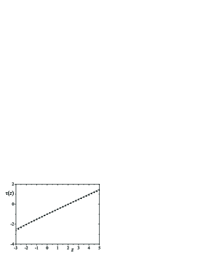
Figure 2: Scaling exponent $\tau$ vs. $z$ of the price fluctuations (upper left), shuffled (upper right), phase randomised (lower left), and shuffled plus phase randomised (lower right) time series of DJIA equities. In all panels, the line $\tau=\frac{z}{2}-1$ represents the theoretical curve for an independent and Gaussian time series. For the shuffled plus phase randomised time series, the points coincide with the curve of a Gaussian time series of independent elements. For the other cases, we verify a departure from the line, proving the multifractal behaviour of price fluctuations.

III.2 Multifractality for instantaneous volatility time series

Albeit volatility is not directly observable, it plays a central role in financial modelling engle-review , and it is usually related to the magnitude of price fluctuations. It is on this quantity that long-lasting covariances associated with asymptotic power-laws are measured. As a matter of fact, the appropriate mimicry of a long-lasting autocorrelation function of the volatility associated with a white noise character of the variable upon study is one of prime challenges in several areas of scientific research. Aiming to appraise its potential multiscaling nature we have performed a MF-DFA analysis on instantaneous volatility time series. The main results are shown in Fig. 3 and Fig. 4. From our analysis, we have verified that there are clear differences between multifractal spectra for price fluctuations and absolute values.

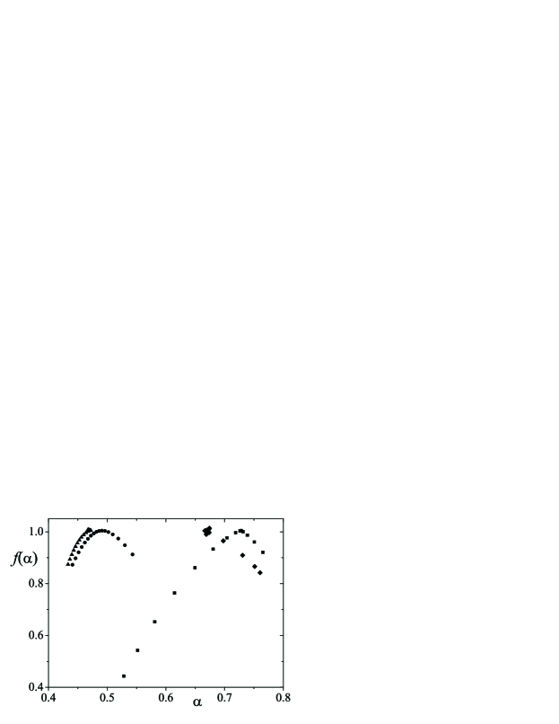
Figure 3: Multifractal spectra $f$ vs. $\alpha$ of the instantaneous volatility ($\blacksquare$), shuffled time series ($\bullet$), phase randomised ($\blacklozenge$), and shuffled plus phase randomised ($\blacktriangle$) time series of DJIA equities. As it is shown, when elements that introduce multi-scaling are removed the multi-fractal spectrum becomes clearly narrower.

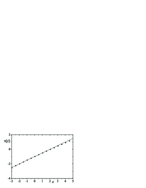
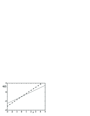
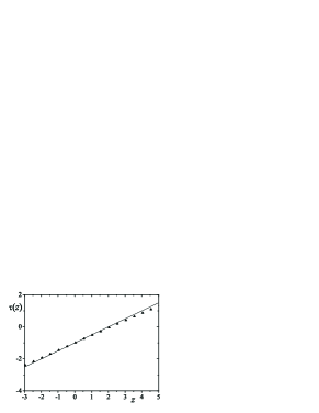
Figure 4: Scaling exponent $\tau$ vs. $z$ of the instantaneous volatility (upper left), shuffled (upper right), phase randomised (lower left), and shuffled plus phase randomised (lower right) time series of DJIA equities. In all panels, the solid line $\tau=\frac{z}{2}-1$ represents the theoretical curve of Gaussian time series of independent elements. Regarding instantaneous volatility results, it is visible the departure from Gaussian independent behaviour that persists when we destroy the Gaussianity. In the lower left panel the dotted line represents the monofractal curve $\tau=H\,z-1$ with $H=h(2)=0.71\pm 0.01$. If we considered the phase randomised time series as a pure monofractal set we would have the best fit for $H=0.692\pm 0.002$, a bit ouside error margin of h(2).

In first place, and against our primary expectations, we have observed that price fluctuations have a wide multifractal spectrum. Specifically, we have computed $\Delta h=0.15$ for price fluctuations, and $\Delta h=0.10$ for volatilities. This corresponds to a ratio of $2$ over $3$. As it happens for price fluctuations, the multifractal spectrum is asymmetric. We have also obtained $h\left(2\right)=0.71$, which indicates a strong persistency on volatility time series in accordance with previous empirical findings. We clarify that we expected to obtain a wider spectrum for instantaneous volatility because of correlations and non-Gaussianity of this quantity. For shuffled instantaneous volatility time series we observe a shift of $f\left(\alpha\right)$, and a lessen of curve width. On the other hand, when we turn instantaneous volatility into a Gaussian variable points multifractal tends do be clearly diminished, though still present. This is in accordance to previous verifications about local fluctuations on Hurst exponent for financial time series cps-volatility which introduce multifractality. Bearing in mind the value $\Delta h=0.10$, the difference between scaling exponents of the shuffled time series, $\Delta h_{shf}=0.05$, points non-Gaussianity and dependence as equally responsible for the multiscaling of instantaneous volatility. From Fig. 4, it is visible that $\tau_{shf}$ almost coincides with the theoretical curve of an independent and Gaussian time series. Such a result indicates that the probability density function presents a nearly exponential decay. We corroborate this result with Fig. 5 in which we present absolute values probability density function, $p\left(v\right)$. In line with Fig. 5 we verify that $p\left(v\right)$ fits for a $F$-distribution,

$$F\left(v\right)\varpropto\left(\frac{v}{\theta}\right)^{\phi}\left[1-\left(1-q\right)\frac{v}{\theta}\right]^{\frac{1}{1-q}},$$ (27)

where $\theta=0.32\pm 0.02$, $\phi=1.83\pm 0.01$, and $q=1.08\pm 0.02$. Taking into account error margins, the small deviation from exponential decay given by numerical adjustment is in agreement with the slight deviation of $\tau_{shf}$ from the theoretical curve that we have measured.

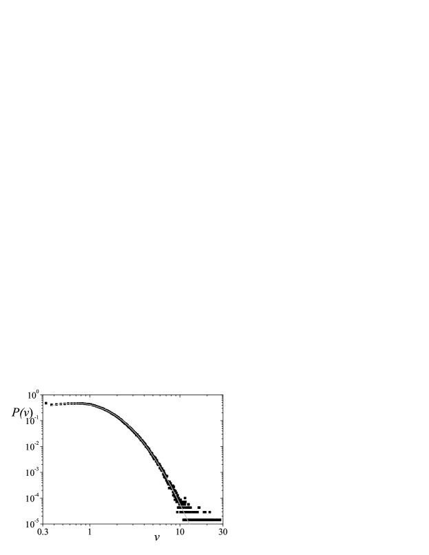
Figure 5: Instantaneous volatility probability density function $P\left(v\right)$ vs. $v$ averaged over DJIA equities. Symbols are the empirical PDF and the line the best fit using a $F$-distribution, Eq. (27) ($\chi^{2}/n=4.4\times 10^{-6}$ and $R^{2}=0.999$).

III.3 Effects of the signal and (instantaneous) volatility multifractal behaviour on price flctuations multiscaling

In this subsection we assess the influence of the multifractal character of instantaneous volatility on the multifractal nature of price fluctuations. To that, we have proceeded the following way. We have separated price fluctuations, $r\left(t\right)$, considering each element as the product of elements of two other time series, i.e., one that considers the signal of the price fluctuation, $s\left(t\right)=\pm 1$, and other which takes into account the magnitude or instantaneous volatility, $v\left(t\right)=\left|r\left(t\right)\right|$. Preserving the signal time series, we have multiplied $\left\{s\left(t\right)\right\}$ by time series that were obtained after shuffle, $v_{shf}\left(t\right)$, phase randomisation, $v_{rnd}\left(t\right)$, and shuffle plus phase randomisation, $v_{shf-rnd}\left(t\right)$, procedures. The results we have obtained are depicted in Fig. 6 and Fig. 7. From Fig. 6, we see that the statistical properties of volatility do influence the multifractal spectrum of price fluctuations. If we only shuffle $\left\{v\left(t\right)\right\}$ elements, the $u\left(t\right)$ time series,

$$u\left(t\right)\equiv s\left(t\right)\,v\left(t\right),$$

just has a paltry narrower $f\left(\alpha\right)$ curve than $\left\{r\left(t\right)\right\}$. It has $\Delta h=0.13$ in opposition to $\Delta h=0.15$ of $\left\{r\left(t\right)\right\}$. This is an unexpected result regarding the influence of $\left\{v\left(t\right)\right\}$ ordering on its multifractal spectrum. However, when we destroy the non-Gaussianity of instantaneous volatility probability density function, we basically destroy the multifractal spectrum of price fluctuations, since $\Delta h=0.04$, or $\Delta h=0.03$ when we combine shuffling with phase randomisation procedures on $\left\{v\left(t\right)\right\}$. The latter result also sets the influence of the signal ordering on the price fluctuations multifractal character at the order of error in absolute accordance with previous analysis for other characteristics, namely the approach to the Gaussian when of cummulative price fluctuations probability density functions lyra .

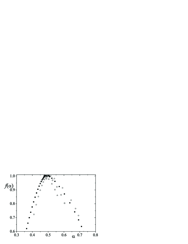
Figure 6: Multifractal spectra $f$ vs. $\alpha$ of the price fluctuations ($\blacksquare$), and of time series $\left\{r\left(t\right)\right\}$ that use shuffled ($\circ$), phase randomised ($\Diamond$), and shuffled plus phase randomised ($\triangle$) volatility time series of DJIA equities. As it is depicted, the multifractal character of volatility plays an essential role at the multifractal nature of price fluctuations. This role is clear for the non-Gaussianity of $v\left(t\right)$.

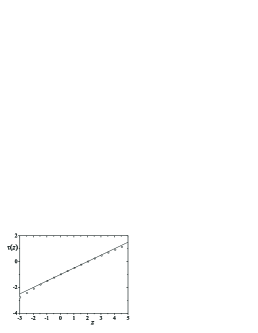
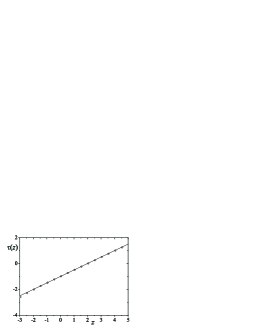
Figure 7: Scaling exponent $\tau$ vs. $z$ of time series $\left\{r\left(t\right)\right\}$ that use shuffled (right), phase randomised (centre), and shuffled plus phase randomised (left) volatility time series of DJIA equities. In all panels, the line $\tau=\frac{z}{2}-1$ represents the theoretical curve for an independent and Gaussian time series. The importance of the multifractal characteristics of volatility are demonstrated by the clear approach of these three results towards the theoretical curve of an independent Gaussian process.

As it has been observed bouchaud smdq-qf , many of the dynamical and statistical properties of price fluctuations depend on the volatility. Although it is a pivotal variable in finance the truth is that volatility definition is still ambiguous engle-gallo . If in many situations it is presented has we have been doing, volatility is oftenly determined as the standard deviation of price fluctuations over window of length $l$ . The latter definition is widely applied on stochastic volatility models. In that particular case, superstatistical models have been applied in problems of financial origin bouchaud sato to define such models. Concisely, superstatistics or “statistics of statistics” beck-cohen is a compound method which has emerged within statistical mechanics. It is based on the assumption of a local statistics dependent on a parameter that fluctuates (smoothly) on a time scale that is very large when compared with the time needed for a system to reach a local equilibrium or stationarity. In a superstatistical context it has been proved that, if we have a set of local Gaussian random variables,

$$\mathcal{G}_{\sigma}\left(x\right)=\frac{1}{\sqrt{2\pi}\sigma}\exp\left[-\frac{x^{2}}{2\,\sigma^{2}}\right],$$ (28)

and the inverse variance, $\sigma^{-2}$, is associated with a $\Gamma$-distribution,

$$\Gamma\left(x\right)\varpropto\left(\frac{x}{\delta}\right)^{\gamma}\exp\left[-\frac{x}{\delta}\right],$$ (29)

then, the stationary distribution given by

$$p\left(x\right)=\int\mathcal{G}_{\sigma}\left(x\right)\,\Gamma\left(\sigma^{-2}\right)\,d\left(\sigma^{-2}\right),$$

is equal to a Tsallis (or Student $t$-) distribution tsallis-milan ,

$$p\left(x\right)=\frac{1}{Z}\left[1-\left(1-q\right)\,\frac{x^{2}}{\lambda}\right]^{\frac{1}{1-q}},$$ (30)

where

$$q=1+\frac{2}{3+2\,\gamma}.$$ (31)

In this way, superstatistics has been considered has the first dynamical foundation for non-extensive framework beck-prl that has non-additive entropy, $S_{q}$ ct , as its cornerstone. Distribution (30) has regularly been used to fit for price fluctuations of several financial markets, and also for the data set we have been analysing for which it has been found a value of $q=1.31\pm 0.02$ canberra . If we assume a superstatistical approach for the data set upon analysis from Eq. (31) we obtain $\gamma=1.82$.

In what follows we analyse a discrete $ARCH$-like process engle-arch that can be catalogued as superstatistical. Explicitly, we have generated time series, $\left\{y\left(t\right)\right\}$, from the product of an uncorrelated Gaussian signal, $\left\{\omega\left(t\right)\right\}$, with $\left\langle\omega\left(t\right)\right\rangle=0$, and $\left\langle\omega\left(t\right)^{2}\right\rangle=1$ by an uncorrelated volatility signal, $\left\{\sigma\left(t\right)\right\}$,

$$y\left(t\right)\equiv\sigma\left(t\right)\,\omega\left(t\right),$$

such that $\sigma^{-2}$ follows a $\Gamma$-distribution with $\gamma=1.82$ as we have obtained. In this case, because we neglect memory on volatility, we can compare the multifractal study of this time series with the results that we have presented at the beginning of this subsection III.3 for $\left\{u\left(t\right)\right\}$ with a shuffled instantaneous volatility. We have opted for this comparison because, just as $s\left(t\right)$, $\omega\left(t\right)$ does not contribute to the multifractal spectrum. The excerpt of the time series we have generated is presented in Fig. 8. In the same figure we comprove that $\left\{y\left(t\right)\right\}$ follows PDF (30) with $q=1.3$.

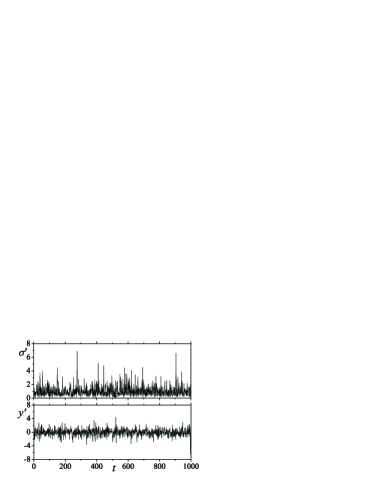
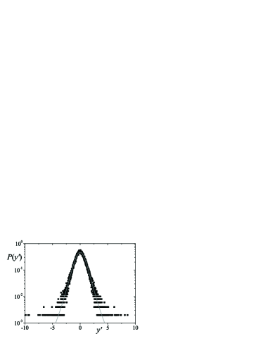
Figure 8: Left: Excerpt of the $ARCH$-like signal (lower panel) where $y^{\prime}$ represents $y$ divided by the average value of $\sigma$, $\sigma_{m}$. The elements of $\sigma$ signal (upper panel) follow a PDF such that $P\left(\sigma^{-2}\right)$ is a $\Gamma$-distribution with $\gamma=1.82$, and $\delta=2$. Right: Stationary PDF of $y^{\prime}$, $P\left(y^{\prime}\right)$ vs. $y^{\prime}$. Symbols have been obtained from the time series and the line is the numerical adjustment for a $q$-Gaussian distribution with $q=1.3$. Although this is not an exact approach, the adjustment is rather nice ($\chi^{2}/n=1.2\times 10^{-5}$ and $R^{2}=0.99$).

Afterwards, we have performed a multifractal analysis along the same lines we have made for price fluctuations. Even though both multifractal spectra are very similar we can verify a noticeable difference. As a matter of fact we have obtained $\Delta\alpha=0.28$ for $\left\{y\left(t\right)\right\}$ with shuffled volatility time series, and $\Delta\alpha=0.24$ for the generated series that we have priory analysed, i.e., an error of $17\%$, see in Fig. 9. This means that superstatistics can be considered as an acceptable first approach, although models that consider long term memory in variance qarch are certainly more appropriate. Since the only source of multifractality in this case is the asymptotic power-law behaviour of the stationary PDF $P\left(y\right)$, $\left\{y\left(t\right)\right\}$ should be in fact called a bifractal with $\tau\left(z\right)=0$ for $z>5.45$.

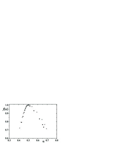
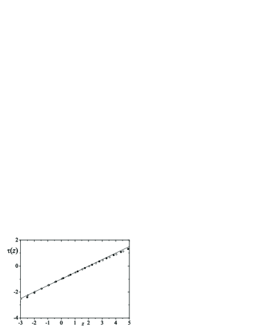
Figure 9: Left panel: Multifractal spectra $f$ vs. $\alpha$ of the $\left\{y\left(t\right)\right\}$ ($\bullet$), and of time series $\left\{r\left(t\right)\right\}$ that use shuffled ($\circ$) volatility time series of DJIA equities. Right panel: Scaling exponent $\tau$ vs. $z$ of $\left\{y\left(t\right)\right\}$ ($\bullet$) and of time series $\left\{r\left(t\right)\right\}$ that use shuffled ($\circ$) volatility time series of DJIA equities. The line $\tau=\frac{z}{2}-1$ represents the theoretical curve for an independent and Gaussian time series.

IV Results for $\ell$-diagrams 

A rich and interesting way of representing time series is to consider a mapping of the time series onto a plane where each point signalled is obtained by pairing elements $x_{t}$ and $x_{t+\ell}$ of the time series as ordinate and abcissa, respectively. This $\ell$-diagrams and related methods rp are frequently used on studies about biological ldv , and dynamical systems rp . Moreover,  they have also been introduced to study daily fluctuations of some securities ausloos-return . This type of representation, full called as $\ell$-diagram variability method ldv , is in fact quite illustrative since it is a simple way of capturing regular aspects of systems which are apparently irregular. Such regularities can be characterised by regions which are more visited in space $x_{t}\times x_{t+\ell}$. Specifically, taking into account price fluctuations time series and $\ell=1$ as an example, it allows one to verify how prices evolve in segments of two time intervals. Nextly, we analyse the first return map of the price fluctuations. In Fig. 10 we show the plot of $r_{t+1}$ versus $r_{t}$ for some of the companies of our set . The plots present a very interesting structure. Over the four quadrants (anticlockwise) we have got stripes with high density of points and “forbidden” regions close to the axes. We assign to transaction costs the emergence of this banned regions. In the $3^{rd}$ quadrant we can see a highly visited region close to the origin, point that small decreases induce small decreases. We have investigated the probabilities for each quadrant and we have found a very peculiar behaviour for DJ30 . The probabilities for each quadrant (anticlockwise) can be interpreted as follows: $1^{st}$ quadrant - probability of two consecutive profits, $P_{1}$; $2^{nd}$ quadrant - probability of a profit after a loss, $P_{2}$; $3^{rd}$ quadrant - probability of two consecutive loss, $P_{3}$; $4^{th}$ quadrant - probability of a loss after profit, $P_{4}$. These results are shown in Table 1. As it is easily observable the dynamics of the system is basically up-and-down-and-up since the fourth and second quadrants together represent $2/3$ of the points plotted on 1-diagrams, with the probabilities of having either two consecutive profits or two consecutive losses equal to $17\%$, in average. Interestingly, we have verified that although the number of negative price fluctuations surpasses the number of positive price fluctuations, $N\left(r_{i}>0\right)-N\left(r_{i}<0\right)=-199$ (related to the skewness of the distributions), the cumulative sum of price fluctuations yields a positive value for all equities, $\sum_{t}r_{i}\left(t\right)=3.82$ (in average). In other words, although during the period upon analysis there was a larger number of negative price fluctuations than positive price fluctuations, the magnitude of the latter were greater so that a positive evolution arose. As a matter of fact, during this period the DJIA index increased its magnitude from $10334.16$ to $10783.01$, or a heighten of $4.8\%$.

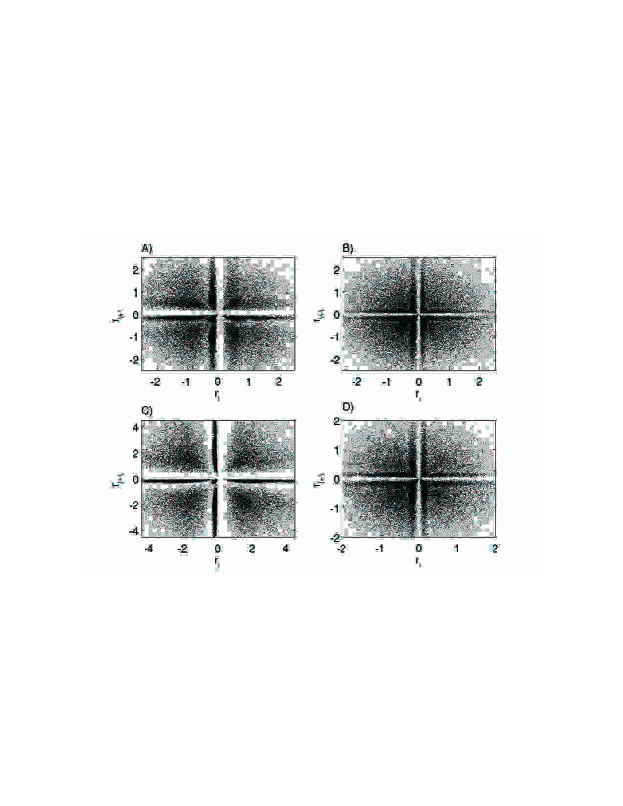
Figure 10: Recurrence maps (step $s=1$) for the companies Caterpilar (A), Citibank (B), Intel (C) and 3M (D) - detrended data.($i\equiv t$)

Be aware that, looking at Fig. 10, there exists a clear pattern for these probabilities. In order to further show that these characteristic patterns go beyond the uncorrelated essence of price fluctuations time series, we have performed immediate $1$-diagrams for the shuffled signals. The results are presented in Fig. 11 where it is visible that these diagrams are different from the diagrams that we have shown in Fig. 10, namely the accumulation around lines $r_{t+1}=\pm r_{t}$ becomes less clear. Furthermore, analysing shuffled plus randomised times series, Fig. 12, we have observed the lost of any pattern, forbidden stripes inclusive. Actually, both of the two latter representations are more homogeneous. In our opinion this is a clear evidence about the importance of dependencies and non-Gaussianity on price fluctuations dynamics. At this point it is absolutely necessary to stress that this profile for $1$-diagrams does not contradics the EMH, if one tried to make use of this property for immediate trading, transaction costs would surpass any possible (read likely) income.

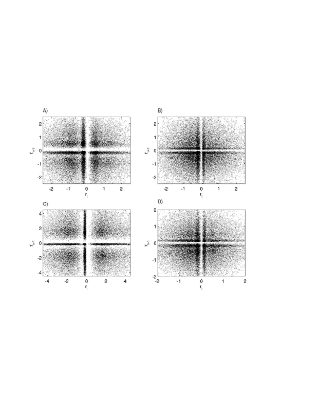
Figure 11: Recurrence maps (step $s=1$) for the companies Caterpilar (A), Citibank (B), Intel (C) and 3M (D) - detrended and shuffled data.($i\equiv t$)

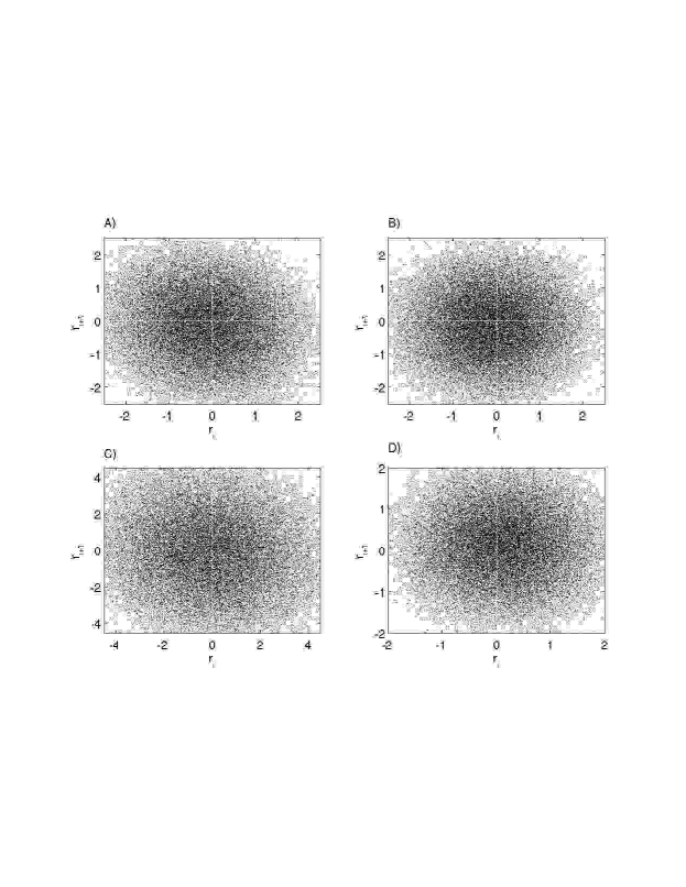
Figure 12: Recurrence maps (step $s=1$) for the companies Caterpilar (A), Citibank (B), Intel (C) and 3M (D) - detrended, shuffled plus phase randomised data.($i\equiv t$)

Table 1: Probabilities for each quadrant (columns 2-4) of 30 companies of the DJ30. In column 6 is shown the difference between positives price fluctuations and negative price fluctuations, and in column 7 is shown the sum of all returns. The last two columns have been obtained from trended data. Even though most price fluctuations are negative (for most companies) though the sum is positive. Note also that there is a clear pattern for the quadrants for the 30 companies.

	$P_{1}\quad$	$P_{2}\quad$	$P_{3}\quad$	$P_{4}\quad$	$N\left(r_{i}>0\right)-N\left(r_{i}<0\right)\quad$	$\sum r_{i}$
aa	0.17	0.33	0.17	0.33	-269	4.99
aig	0.18	0.33	0.17	0.33	-55	4.16
axp	0.18	0.33	0.17	0.33	-157	1.38
ba	0.18	0.33	0.17	0.33	-262	4.01
c	0.18	0.33	0.16	0.33	132	4.80
cat	0.17	0.33	0.18	0.33	-477	6.55
dd	0.18	0.33	0.17	0.33	-130	5.09
dis	0.17	0.33	0.17	0.33	-237	5.02
ge	0.17	0.33	0.17	0.33	-280	4.71
gm	0.18	0.33	0.17	0.33	-366	2.92
hd	0.18	0.33	0.17	0.33	-113	0.76
hon	0.18	0.33	0.17	0.33	-269	1.11
hpq	0.17	0.33	0.17	0.33	10	5.34
ibm	0.18	0.32	0.17	0.32	-45	0.90
intc	0.19	0.32	0.18	0.32	172	2.23
jnj	0.17	0.33	0.17	0.33	-96	0.57
jpm	0.17	0.33	0.17	0.33	-276	0.76
ko	0.18	0.33	0.17	0.33	-289	6.22
mcd	0.18	0.33	0.16	0.33	33	1.15
mmm	0.18	0.33	0.16	0.33	-348	7.23
mo	0.18	0.33	0.16	0.33	-82	6.17
mrk	0.17	0.33	0.17	0.33	-298	1.16
msft	0.19	0.31	0.18	0.32	-16	1.58
pfe	0.17	0.33	0.17	0.32	-162	3.63
pgn	0.18	0.33	0.17	0.33	-62	5.16
sbc	0.18	0.32	0.17	0.33	-336	6.54
utx	0.18	0.32	0.17	0.33	-478	5.85
vz	0.17	0.33	0.17	0.33	-191	4.65
wmt	0.17	0.33	0.18	0.32	-583	4.03
xom	0.17	0.33	0.17	0.33	-452	6.02
average	0.17	0.33	0.17	0.33	-199	3.82

Analysing $\ell$-diagrams for $\ell=2,4,10$ we have verified an equal occupancy of all quadrants,$P_{1}=P_{2}=P_{3}=P_{4}=25\%,$ which indicates the loss of any predictability on the time series.

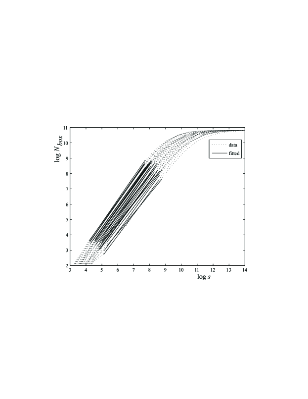
Figure 13: Estimation of the fractal dimension of the $r_{t}\times r_{t+1}$ space using Eq. (18).

To quantify the properties of $\ell$-diagrams we have also applied the algorithm described in Sec. II.3. Namely, we have mapped the space $r_{t}\times r_{t+1}$ onto interval $[2^{0},2^{16}-1]$, and we have estimated the fractal dimension of this space structure for the 30 companies. In Fig. 13 it is noticeable that for the majority of companies the scale regime holds over a large range of scales. We have then used the interval $2^{2}$ to $2^{8}$ to numerically obtain the fractal dimensions that are shown in Table 2, which correspond to the slopes of the fitting straight lines in Fig. 13. Therein, it is verifiable that the fractal dimension vary slight as the step ($s$) is changed, as well as after a shuffling procedure (keeping the order of the diagram). However, it is strongly affected by phase randomization, and it presents for this case values that are compatible with a 2-dimensional Gaussian distribution.

Table 2: Fractal dimension of the $r_{t}\times r_{t+\ell}$ space ($\ell=1,2,10,50$) for the companies of the DJ30 estimated with Hou algorithm.

	$d_{f}\left(\ell=1\right)\quad$	$d_{f}\left(\ell=2\right)\quad$	$d_{f}\left(\ell=10\right)\quad$	$d_{f}\left(\ell=50\right)\quad$	$d_{f}\left(\ell=1\right)$ (shuf.)	$d_{f}\left(\ell=1\right)$ (rand)
aa	1.45	1.42	1.43	1.45	1.45	1.68
aig	1.28	1.25	1.26	1.29	1.40	1.67
axp	1.46	1.44	1.45	1.44	1.45	1.67
ba	1.44	1.45	1.43	1.44	1.45	1.67
c	1.33	1.31	1.31	1.31	1.33	1.67
cat	1.37	1.37	1.36	1.41	1.41	1.67
dd	1.45	1.47	1.47	1.48	1.47	1.66
dis	1.50	1.50	1.50	1.51	1.51	1.66
ge	1.52	1.53	1.54	1.51	1.52	1.66
gm	1.46	1.43	1.46	1.45	1.46	1.67
hd	1.37	1.39	1.37	1.39	1.36	1.68
hon	1.48	1.46	1.48	1.47	1.48	1.67
hpq	1.46	1.46	1.47	1.47	1.50	1.67
ibm	1.43	1.47	1.44	1.45	1.45	1.64
intc	1.35	1.40	1.40	1.43	1.41	1.69
jnj	1.36	1.36	1.37	1.37	1.41	1.65
jpm	1.44	1.44	1.41	1.44	1.43	1.67
ko	1.46	1.44	1.45	1.44	1.45	1.67
mcd	1.44	1.45	1.43	1.44	1.45	1.67
mmm	1.33	1.31	1.31	1.31	1.33	1.67
mo	1.37	1.37	1.36	1.41	1.41	1.67
mrk	1.45	1.47	1.47	1.48	1.47	1.66
msft	1.50	1.50	1.50	1.51	1.51	1.66
pfe	1.52	1.53	1.54	1.51	1.52	1.66
pgn	1.46	1.43	1.46	1.45	1.46	1.67
sbc	1.37	1.39	1.37	1.39	1.36	1.68
utx	1.48	1.46	1.48	1.47	1.48	1.67
vz	1.46	1.46	1.47	1.47	1.50	1.67
wmt	1.43	1.47	1.44	1.45	1.45	1.64
xom	1.35	1.40	1.40	1.43	1.41	1.69

V Final remarks

To summarise, in this manuscript we have made an exhaustive analysis of the effective multifractal properties of high-frequency price fluctuations and instantaneous volatility of the equities that compose Dow Jones Industrial Average. This analysis has comprised the quantification of dependence and non-Gaussianity on the multifractal character of price fluctuations and volatility. Furthermore, we have studied the multifractal properties of the $\ell$-diagrams made from price fluctuations time series. Our results indicate that dependence and non-Gaussianity have similar weights on the multifractal features of both financial quantities. Contrarily to some stylised facts, and especially for instantaneous volatility cps-volatility , we have not verified a solid asymptotic power-law decay of the probability density functions, i.e., fair deviations from exponential decay. This result is substantiated by the clear approach of $\tau\left(z\right)$ curves to the theoretical curve of a independent gaussian signal when we perform a shuffling on time series elements. If we consider persistence as a major factor for multiscaling, it might be puzzling to verify that multifractality for price fluctuations is stronger than it is for magnitude price fluctuations. Such an apparent contradiction is cleared up if we take into consideration that price fluctuations PDF appears to be more fat tailed than instantaneous volatility which introduces a larger contribution to multiscaling. Besides, in respect of probability density functions, we have observed that a superstatistical approach to price fluctuations appears to be valid as a first approach. Still on multiscaling, we have tried to appraise the robustness of instantaneous volatility by means of measuring the effect of its possible multifractal nature on price fluctuations multifractal properties. Our results have indicated that the non-Gaussinity of instantaneous volatility (price fluctuation magnitudes) is the chief element of multifractal properties of price fluctuations. This occurs because the uncorrelated character of the signal annihilates the influence of dependences of instantaneous volatility leading to the non-Gaussianity of latter quantity the chief role of introducing multifractality on price fluctuations time series. In this perspective heteroskedastic (i.e., $ARCH$) approaches, within superstatistics is enclosed, to price fluctuations are validated.

Analysing $\ell$-diagrams obtained from price fluctuations time series we have got sequences of immediate price fluctuations around Cartesian axes that are forbidden. We have attributed this fact to transaction costs. We have also observed that despite the number of negative price fluctuations is greater than the number of positive price fluctuations, the sum all returns is in fact positive, which is in accordance with both price fluctuations skewness and economical evolution. By means of a box counting algorithm we have computed the fractal dimension of such diagrams. We have verified that the fractal dimension varies slightly when time ordering is destroyed, and it is deeply affected by randomisation procedures. This provides an important clue on the fundamental role of non-Gaussinity of price fluctuations in several properties usually observed.

Acknowledgements

We would like to thank L.G. Moyano who has performed the intraday pattern removal described in Sec. II, as well as E.M.F. Curado and C. Tsallis for their several comments on the matters which are enclosed in this manuscript. One of us (JdS) acknowledges support of S.P. Rostirolla and F. Mancini. The code for estimating multifractal spectrum of time series was written during JdS visit to The Abdus Salam International Centre for Theoretical Physics, Trieste - Italy. The data used was provided by Olsen Data Services to whom we are also grateful. We appreciate the useful remarks from M.L. Lyra and R.L. Viana at the final stage of the work. This work has benefited from infrastructural support from PRONEX and PETROBRAS, and financial support from CNPq (Brazilian agency) and FCT/MCES (Portuguese agency).

References

- (1) B.B. Mandelbrot, The Fractal Geometry of Nature (W. H. Freeman & Co., San Francisco, 1983).
- (2) M. Gell-Mann, The Quark and the Jaguar, Adventures in the Simple and the Complex (W. H. Freeman & Co., San Francisco, ); A.T. Skjeltrop and T. Vicsek, Complexity from the Microscopic to Macroscopic Scales: Coherence and Large Deviations (Kluwer Academic Publishers, Dordrecht, 2002).
- (3) C.-K. Peng, J. Mietus, J. M. Hausdorff, S. Havlin, H. E. Stanley, and A. L. Goldberger, Phys. Rev. Lett. 70 (1993) 1343.
- (4) J. M. Hausdorff, P. L. Purdon, C.-K. Peng, Z. Ladin, J. Y. Wei, and A. L. Goldberger, J. Appl. Physiol. 80 (1996) 1448.
- (5) L.F. Burlaga and A.F. Vinas, Physica A 356 (2005) 375.
- (6) J.-P. Bouchaud and M. Potters, Theory of Financial Risks: From Statistical Physics to Risk Management (Cambridge University Press, Cambridge, 2000).
- (7) R.N. Mantegna and H.E. Stanley, An introduction to Econophysics: Correlations and Complexity in Finance (Cambridge University Press, Cambrigde, 1999).
- (8) J. Feder, Fractals (Plenum, New York, 1988).
- (9) B.B. Mandelbrot, J. Business 36 (1963) 394; B.B. Mandelbrot, Fractals and Scaling in Finance (Springer, New York, 1997)
- (10) I. Andreadis and A. Serletis, Chaos Solit. Fract. 13 (2002) 1309; K. Ivanova and M. Ausloos, Eur. Phys. J. 8 (1999) 665; T. Di Matteo, Quant. Financ. 7 (2001) 21.
- (11) A. Admati and P. Pfleiderer, Rev. Financial Studies 1 (1988) 3.
- (12) J. W. Kantelhardt, S. A. Zschiegner, E. Koscielny-Bunde, S. Havlin, A. Bunde, and H.E. Stanley, Physica A 316 (2002) 87.
- (13) P. Ch. Ivanov, L.A.N. Amaral, A.L. Goldberger, S. Havlin, M.G. Rosenblum, H.E. Stanley, and Z.R. Struzik, Chaos 11 (2001) 641; K. Matia, Y. Ashkenazy, and H.E. Stanley, Europhys. Lett. 61 (2003) 422; Y. Ashkenazy, D.R. Baker, H. Gildor, and S. Havlin, Geophys. Res. Lett. 30 (2003) 2146 ; L. Telesca, V. Lapenna, and M. Macchiato, New J. Phys. 7 (2005) 214.
- (14) A. Kruger, Comput. Phys. Commun. 98 (1996) 224.
- (15) J. de Souza and S.P. Rostirolla, A fast MATLAB® program to estimate the multifractal spectrum of multidimensional data: application to fractures. (preprint, 2007).
- (16) L.G. Moyano, J. de Souza, and S.M. Duarte Queirós, Physica A 371 (2006) 118.
- (17) S.M. Duarte Queirós, L.G. Moyano, J. de Souza, and C. Tsallis, Eur. Phys J. B 55 (2007) 161.
- (18) J.F. Muzy, E. Bacry, A. Arneodo, Phys. Rev. Lett. 67 (1991) 3515.
- (19) P. Oświȩcimka, J. Kwapień, and S. Drożdż, Phys.Rev. E 74 (2006) 016103.
- (20) H. E. Hurst, Trans. Am. Soc. Civ. Eng. 116 (1951) 770.
- (21) C.-K. Peng, S.V. Buldyrev, S. Havlin, M. Simons, H.E. Stanley, and A.L. Goldberger, Phys. Rev. E 49 (1994) 1685.
- (22) X.-J. Hou, R. Gilmore, G.B. Mindin, and H.G. Solari, Phys. Lett. A 151 (1990) 43.
- (23) L.S. Liebovitch and T. Toth, Phys. Lett. A 141 (1989) 386.
- (24) C. Meneveau and K.R. Sreenivasan, Phys. Rev. Lett 59 (1987) 1424.
- (25) E.-F. Fama, J. Finance 25 (1970) 383.
- (26) D.K. Umberger and J.D. Farmer, Phys. Rev. Lett 55 (1985) 661.
- (27) W. Feller, Probability theory and its applications (John Wiley, New York, 1950).
- (28) A. Serletis and M. Shintani, Chaos Solit. Fract. 17 (2003) 449; J. de Souza, L.G. Moyano and S.M. Duarte Queirós, Eur. Phys. J. B 50 (2006) 165.
- (29) S.M. Duarte Queirós, Quant. Finance 5 (2005) 475.
- (30) C. Granger, and J. Lin, J. Time Ser. Anal. 15 (1994) 371; L. Borland, A.R. Plastino, C. Tsallis, J. Math. Phys. 39 (1998) 6490.
- (31) R.F. Engle and A.J. Patton, Quant. Finance 1 (2001) 237; P. Embrechts, C. Kluppelberg, and T. Mikosch, Modelling Extremal Events for Insurance and Finance (Applications of Mathematics) (Springer-Verlag, Berlin, 1997).
- (32) R.F. Engle and G.M. Gallo, J. Econometrics 131 (2006) 3
- (33) M. Kozaki and A.-H. Sato, Physica A (2007), doi:10.1016/j.physa.2007.10.023
- (34) C. Beck and E.G.D. Cohen, Physica A 322, 267 (2003).
- (35) C. Tsallis, Milan J. Math. 73 (2005) 145.
- (36) E.G.D. Cohen, Pramana - J. Phys. 64 (2005) 635.
- (37) C. Tsallis, J. Stat. Phys. 52 (1988) 479.
- (38) R.F. Engle, Econometrica 50 (1982) 987.
- (39) S.M. Duarte Queirós, EPL 80 (2007) 30005.
- (40) G.M. Viswannathan, U.L. Fulco, M.L. Lyra, and M. Serva, Physica A 329 (2003) 273.
- (41) E.M. Stein and J.C. Stein, Rev. Fin. Stud. 4 (1991) 727.
- (42) A. Babloyantz, P. Maurer, Phys. Lett. A 221 (1996) 43.
- (43) N. Marwan, M.C. Romano, M. Thiel, and J. Kurths, Phys. Rep. 438 (2007) 237.
- (44) K. Ivanova and M. Ausloos, Physica A 265 (1999) 279.
- (45) Y. Liu, P. Gopikrishnan, P. Cizeau, M. Meyer, C.-K. Peng, H.E. Stanley, Phys. Rev. E 60 (1999) 1390.