Numerical simulations of possible finite time singularities in the incompressible Euler equations: comparison of numerical methods

Abstract

The numerical simulation of the 3D incompressible Euler equation is analyzed with respect to different integration methods. The numerical schemes we considered include spectral methods with different strategies for dealiasing and two variants of finite difference methods. Based on this comparison, a Kida-Pelz like initial condition is integrated using adaptive mesh refinement and estimates on the necessary numerical resolution are given. This estimate is based on analyzing the scaling behavior similar to the procedure in critical phenomena and present simulations are put into perspective.

I Introduction

The question, whether the incompressible Euler equations develop singularities in finite time starting from smooth initial conditions, remains an outstanding open problem in applied mathematics. Although substantial progress has been made in recent years using a more geometrical viewpoint constantin-fefferman-etal:1996 ; gibbon:2002 ; gibbon:2007 ; deng-hou-etal:2005 ; deng-hou-etal:2006 , it is yet not clear from numerical simulations, whether the assumptions of the theorems for non-blow up are fulfilled for flows evolving from simple smooth initial conditions. Singular structures, evolving in finite time or simply “fast enough”, may play a similar role as shock-like structures in compressible flows, providing structures which dominate the energy dissipation even in the non-viscous situation (see Eyink eyink:1994 ; eyink-sreenivasan:2006 ; eyink:2007 and references therein).

In this paper, we study a Kida-Pelz like flow with different numerical schemes: spectral methods with different strategies of dealiasing (this extends the study of Hou and Li hou-li:2007 and confirms their results), two finite difference methods and a finite volume method. Studying the structures of vorticity, it turns out that the differences between the various methods of dealiasing are more pronounced than between the spectral methods and the finite difference/volume methods. This result suggests that resolving the vorticity structures is more important than the order of the numerical scheme. It also justifies the use of finite difference/volume methods in adaptive mesh refinement (AMR) simulations to resolve the vorticity structures.

Using AMR simulations up to an effective resolution of $4096^{3}$ mesh points and comparing the results to lower resolution runs, we observe that the standard way of presenting a $1/|{\bm{\omega}}|$ plot in time may lead to misleading conclusions. However, looking at normalized plots reveals the issue of numerical resolution in a convincing manner.

II Numerical schemes

In this section we compare spectral methods with different dealiasing and finite difference/volume methods.

II.1 Spectral methods and dealiasing

We use a standard spectral method where the time stepping is performed with a strongly stable 3rd-order Runge-Kutta method shu-osher:1988 in Fourier space and where nonlinearities are calculated in real-space. On Linux-clusters, the FFTW-library is used whereas the library P3DFFT pekurovski-yeung-etal:2006 from the San Diego Supercomputer Center is used on the IBM Regatta series and on BlueGene/L.

We use three ways of dealiasing the spectral data:

1. Spherical mode truncation: this is used in turbulence simulations (Biskamp and Müller biskamp-mueller:1999 ). The spherical mode truncation puts a sphere of radius $\frac{N}{2}$ in Fourier space and nullifies all modes outside this sphere.

2. Standard 2/3 rule: same as above, but using a radius of $\frac{2}{3}\frac{N}{2}=\frac{N}{3}$ canuto-hussaini-etal:1987 . This is the most common way of dealiasing spectral data.

3. High-order exponential cut-off: this method was introduced by Hou and Li hou-li:2007 and consists of introducing a high-order exponential filter function $\rho(k)=\exp(-\alpha(|k|/N)^{m})$ with $\alpha=36$ and $m=36$.

II.2 Finite difference/volumes methods

All presented finite difference/volume methods are second order and use the same strongly stable 3rd-order Runge-Kutta method shu-osher:1988 as used in the spectral simulations.

We implemented three different versions of real-space methods:

1. Staggered grid formulation of Harlow and Welsh harlow-welsh:1965 : Normal components of the velocity are located at their respective cell faces and the pressure is defined at the cell centers. This allows a exact Hodge-decomposition such that no pressure oscillations occur. In addition, it conserves momentum and energy and could thus also been seen as a finite volume method.

2. Vorticity formulation for AMR: From our previous AMR studies grauer-marliani-etal:1998 ; grauer-marliani:2000 we know that the coarse-fine grid interpolations are very sensitive in the 3D Euler simulations. As in the former simulations we choose to perform all data exchange and interpolation using the vorticity ${\bm{\omega}}=\nabla\times\mathbf{u}$. Here, the vorticity is defined at cell centers and we applied a tri-cubic interpolation for coarse-fine grid interpolation. Then, three Poisson equations are solved for the cell-centered vector Potential $\mathbf{A}$ and staggered values for the velocity $\mathbf{u}=\nabla\times\mathbf{A}$ are obtained.

3. Finite volume method: this method is similar to the former but a finite volume method bell-colella-etal:1989 ; bell-marcus:1992b ; grauer-marliani-etal:1998 is used instead of finite differences.

II.3 Comparison

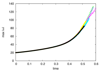
Figure 1: Growth of $\max|{\bm{\omega}}|$ for all implemented numerical schemes.

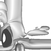
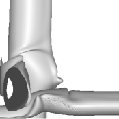
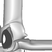
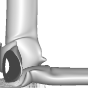
Figure 2: Isosurface plots of vorticity. From top to bottom: spherical truncation, 2/3 rule, exponential filtering, Harlow-Welsh, vorticity formulation, $512^{3}$ mesh points

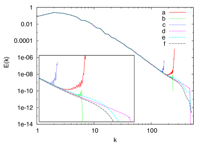
Figure 3: Energy spectra at time $t=0.5$ for spectral and finite difference methods: a) spherical model truncation ($512^{3}$), b) high-order exponential cut-off ($512^{3}$), c) $2/3$ rule ($512^{3}$), d) high-order exponential cut-off ($1024^{3}$), e) vorticity formulation ($1024^{3}$), f) staggered grid formulation ($1024^{3}$)

We first compare the growth of the maximum vorticity according to the Beale-Kato-Majda result beale-kato-etal:1984 ; ponce:1985 for all six numerical methods described above. The initial condition was chosen similar to Kida-Pelz 12 vortices kida:1985 ; boratav-pelz:1994 ; pelz:2001 with a Gaussian shape for the vorticity distribution. Resolution of all the spectral simulations were $512^{3}$ mesh points (corresponding to the full domain) and in addition the Hou-Li exponential filtering was repeated with $1024^{3}$ mesh points. The finite difference/volume simulations were performed with $512^{3}$ and $1024^{3}$ mesh points. The growth of $\max|{\bm{\omega}}|$ is shown in Fig. 1. All simulation agree very well up to the time when the flow is underresolved. This is about $t=0.4$ for the simulations using $512^{3}$ mesh points and $t=0.47$ for the $1024^{3}$ runs. There is no particular criterion which simulation performs better once the simulation is underresolved. The very simple message from this comparison is: you just have to resolve the flow and this is more important than the order of the scheme.

In order to display the differences and similarities of the various numerical methods, we used a “low resolution” simulation with $512^{3}$ mesh points at a late time $t=0.5$ where the flow is already underresolved. Therefore, we looked at very low levels ($5\%$ of the maximum vorticity) as suggested and done by Kerr kerr:2006 and Hou and Li hou-li:2006 . Due to the high symmetry of the flow, only $1/8$ of the total configuration is shown. (To get a better impression for the geometry of the vortices, see Fig. 4, which shows an isosurface of $70\%$ of the peak vorticity.)

The spherical truncation produces highly visible artifacts due to heavy oscillations which grow to substantial values. This is mostly suppressed in the simulation using the classical $2/3$ rule and nearly vanishes for the high order exponential smoothing. Thus our comparison confirms the analysis of Hou and Li hou-li:2006 . Remarkable is the strong similarity of the real-space methods to the spectral simulation with high order exponential smoothing. This is especially visible in Fig. 3, which shows the energy spectrum for spectral and finite difference/volume methods at time $t=0.5$. In the spectral schemes, the spherical truncation and the 2/3 rule show a strong Gibbs phenomena which is absent in the exponential filtering and the finite difference/volume schemes. The Harlow-Welsh method is slightly more dissipative than the vorticity formulation. From the comparison with the spectral schemes using exponential filtering and $1024^{3}$ mesh points it is safe to say that the finite difference schemes with an approximately 1.3 times larger resolution in each spatial direction perform equally well as the spectral code with exponential filtering. Thus, our conclusions of this comparison is that the differences in the simulation results caused by the choice of the dealiasing method are larger than the difference to and between the real-space methods. Our finding thus confirms the viewpoint of Orlandi and Carnevale orlandi-carnevale:2007 and justifies the use of finite difference/volume methods as integration scheme in an adaptive mesh refinement treatment.

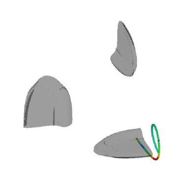
Figure 4: Isosurface plot of $\max|{\bm{\omega}}|$ at $70\%$ of maximum vorticity. Shown is also the trajectory of a particle moving to the position of maximum vorticity.

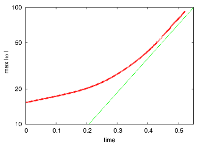
Figure 5: Growth of vorticity along the Lagrangian trajectory (red) which ends near the point of maximum vorticity and a fitted exponential (green).

II.4 Lagrangian trajectories

As pointed out in deng-hou-etal:2005 ; gibbon:2007 , the Lagrangian treatment of vorticity amplification is closely related to the local geometric properties – like curvature and torsion – of vortex lines. In Fig. 4 the trajectory of a Lagrangian tracer particle is shown. To obtain this trajectory, we first identified the spatial position of the maximum vorticity at a late time of the simulation and then traced back the actual trajectory. Fig. 5 shows the temporal evolution of vorticity following this trajectory. A tendency to an exponential growth of vorticity along the trajectory is obvious.

III Adaptive mesh refinement simulations

III.1 The framework racoon

For the adaptive mesh refine calculations, we use our framework racoon dreher-grauer:2004 which is designed for massive parallel computations and scales for hyperbolic systems linearly up to 16384 processors on BlueGene BG/L. However, for the incompressible Euler equations, the pressure resp.  vector potential are solved using an adaptive multigrid method brandt:1977 ; barad-colella:2005 which presently scales only up to 64 processors. Therefore, the present simulations are limited to an effective resolution of $4096^{3}$ mesh points. Parallelization and load-balancing is performed using a space-filling Hilbert curve dreher-grauer:2004 .

Using the framework racoon and the vorticity formulation, we solve the incompressible Euler equations with an effective resolution of $4096^{3}$ mesh points. Fig. 6 shows a volume rendering of vorticity at the latest time $t=0.5$ including the adaptive meshes. Memory consumption is quite moderate using less than 80 GBytes.

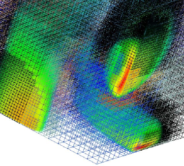
Figure 6: Volume rendering of vorticity at time $t=0.5$.

III.2 Analyzing the growth of vorticity

Looking at Fig. 7 which shows the time evolution of $1/\max|{\bm{\omega}}|$ it is tempting to identify a finite time singularity. However, a more appropriate presentation is obtained plotting $\max|{\bm{\omega}}|\times(t_{0}-t)$ where $t_{0}$ is the expected singularity time. This quantity should converge to a horizontal line in this plot if a singularity occurs in finite time. The time $t_{0}=0.638$ is chosen in a way that this scaling is observed in the late phase of the simulation while the numerics is still resolved.

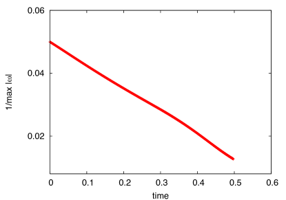
Figure 7: Temporal evolution of $1/\max|{\bm{\omega}}|$.

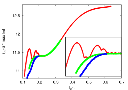
Figure 8: Scaling of the growth of vorticity. Red: $1024^{3}$ mesh points, Blue: $2048^{3}$ mesh points, Green: $4096^{3}$ mesh points. The inlet shows the late phase of the simulation and highlights the importance of numerical resolution.

This is shown in Figs. 8 and the zoom in the inlet of this figure. Especially the zoom of the late phase of the simulation demonstrates, how sensitive the growth of vorticity depends on the numerical resolution and that conclusions drawn from underresolved simulations must be handled with care.

IV Conclusions and Outlook

We demonstrated the extreme sensitivity of the growth of vorticity on the numerical resolution. In order to gain further insight into the mechanism of vorticity amplification, future simulations should include the following analysis and diagnostics: i) If a finite time singularity is expected, then the blow-up time of vorticity must occur at the same time when the spatial position of maximum vorticity and maximum strain come together. ii) The Lagrangian viewpoint should be analyzed according to Deng, Hou and Xu deng-hou-etal:2005 and Gibbon gibbon:2007 . iii) Simulations should use initial conditions including the Kida-Pelz flow kida:1985 and Bob Kerr’s orthogonal tubes kerr:1993 . However, the shape of the initial vortex tube should be chosen in such a way that vortex shedding will not pollute the vorticity growth. For orthogonal vortex tubes this was achieved by Orlandi and Carnevale orlandi-carnevale:2007 starting with Lamb dipoles.