Ultra High Energy Cosmic Rays: origin and propagation

Abstract

We discuss the basic difficulties in understanding the origin of the highest energy particles in the Universe - the ultrahigh energy cosmic rays (UHECR). It is difficult to imagine the sources they are accelerated in. Because of the strong attenuation of UHECR on their propagation from the sources to us these sources should be at cosmologically short distance from us but are currently not identified. We also give information of the most recent experimental results including the ones reported at this conference and compare them to models of the UHECR origin.

1 Introduction

More than forty years ago, in 1963, John Linsley [1] published an article about the detection of a cosmic ray of energy 10²⁰ eV. The article did not go unnoticed, neither it provoked many comments. The few physicists that were interested in high energy cosmic rays were at that time convinced that the cosmic ray energy spectrum will continue forever. The fact that cosmic rays may have energies exceeding 10⁶ GeV (10¹⁵ eV) was established in the late thirties by Pierre Auger and his collaborators. Showers of higher and higher energy were detected in the mean time - seeing a 10²⁰ eV shower seem to be only a matter of time and exposure. Already in the fifties there was a discussion about the origin of such ultra high energy cosmic rays and Cocconi [2] reached the conclusion that they must be of extragalactic origin since the galactic magnetic fields are not strong enough to contain such particles.

How exclusive this event is became obvious three years later, after the discovery of the microwave background radiation (MBR). Almost simultaneously Greisen in US [3] and Zatsepin&Kuzmin [4] in the USSR published papers discussing the propagation of ultra high energy particles in extragalactic space. They calculated the energy loss distance of nucleons interacting in the microwave background and reached the conclusion that it is shorter than the distances between powerful galaxies. The cosmic ray spectrum should thus have an end around energy of 5$\times$10¹⁹ eV. This effect is now known as the GZK cutoff.

The experimental statistics of such events grew with the years, although not very fast. The flux of UHECR of energy above 10²⁰ eV was estimated to be 0.5 to 1 event per square kilometer per century per steradian. Even big detectors of area tens of km² would only detect few events for ten years of work. The topic became one of common interest during the last decade of the last century when ideas appeared for construction of detectors with effective areas in thousands of km² [5, 6]. Such detectors would detect tens of events per year and finally solve all mysteries surrounding UHECR. The Auger observatory (3,000 km²) is now almost fully deployed and the Telescope Array (TA, 1,000 km²) is being constructed in Utah, U.S.A. The expectations for the flux of UHECR are now smaller. The High Resolution Fly’s Eye (HiRes) and Auger have shown that the rate of events above 10²⁰ eV is about 10 times smaller than previously thought.

Cosmic rays are defined as charged nuclei that originate outside the solar system. They come on a featureless, power law like, $F(E)=K\times E^{-\alpha}$, spectrum that extends beyond 10¹¹ GeV per particle. There are only two distinct features in the whole spectrum. At energy above 10⁶ GeV the power law index $\alpha$ steepens from 2.7 to about 3.1. This is called the knee of the cosmic ray spectrum. At energy above 3$\times$10⁹ GeV the spectrum flattens again at the ankle.

The common wisdom is that cosmic rays below the knee are accelerated at galactic supernovae remnants. Cosmic rays above the knee are also thought to be of galactic origin, although there is no clue of their acceleration sites. Cosmic rays above the ankle are thought to be extragalactic.

More recently, with the improved accuracy and exposure of the modern experiments, several theoretical models that fit the measured ultra high energy cosmic rays (UHECR) spectrum have been developed. We will discuss the experimental data and compare them to some of these models.

1.1 Air Shower Detection Methods.

Cosmic rays of energy above 10¹⁴ eV are detected by the showers they generate in the atmosphere. The atmosphere contains more than ten interaction lengths even in vertical direction and is much deeper for particles that enter it under higher zenith angles. It is thus a deep calorimeter in which the showers develop, reach their maximum, and then start being absorbed. There are generally two types of air shower detectors: air shower arrays and optical detectors. Air shower arrays consist of numerous particle detectors that cover large area. The shower triggers the array by coincidental hits in many detectors. The most numerous particles in an air shower are electrons, positrons and photons. The shower also contains muons, that are about 10% of all shower particles, and hadrons.

The direction of the primary particle can be reconstructed quite well from the timing of the different hits, but the shower energy requires extensive Monte Carlo work with hadronic interaction models that are extended orders of magnitude above the accelerator energy range. The main composition sensitive variable is the ratio of the number of muons in the shower N_μ to the number of electrons N_e, or the ratio of muon to electron densities at a certain distance from the shower axis. The type of the primary particles can only be studied in statistically big samples because of the fluctuations in the individual shower development. Even then it is strongly affected by the differences in the hadronic interaction models.

The optical method uses the fact that part of the particle ionization loss is in the form of visible light. All charged particles emit in air Cherenkov light in a narrow cone around their direction. In addition to that charged particles excite Nitrogen atoms in the atmosphere, which emit fluorescence light. The output is not large, about 4 photons per meter, but the number of shower particles in UHECR showers is very large, and the shower can be seen from distances exceeding 30 km. The fluorescence detection is very suitable for UHECR showers because the light is emitted isotropically and can be detected independently of the shower direction. Since optical detectors follow the shower track, the direction of the primary cosmic ray is also relatively easy. The energy of the primary particles is deduced from the total number of particles in the shower development or from the number of particles at shower maximum. The rough number is that every particle at maximum carries about 1.5 GeV of primary energy. The mass of the primary cosmic ray nucleus is studied by the depth of shower maximum $X_{max}$, which is proportional to the logarithm of the primary energy per nucleon.

1.2 The Highest Energy Cosmic Ray Event

Figure 1: The shower profile of the highest energy cosmic ray shower detected by the Fly’s Eye.

The highest energy cosmic ray particle was detected by the Fly’s Eye experiment [7]. We will briefly describe this event to give the reader an idea about these giant air showers. The energy of this shower is estimated to be 3$\times$10²⁰ eV. This is an enormous macroscopic energy. 3$\times$10²⁰ eV is equivalent to 4.8$\times$10⁸ erg, 7.2$\times$10³⁴ Hz or the energy of 290 km/h tennis ball in the favorite units of Alan Watson. Fly’s Eye was the first air fluorescence experiment, located in the state of Utah, U.S.A. Fig. 1 shows the shower profile of this event as measured by the Fly’s Eye. Note that the maximum of this shower contains more than 2$\times$10¹¹ electrons and positrons. Both the integral of this shower profile and the number of particles at maximum give about the same energy.

The errors of the estimates come from the errors of the individual data points, but mostly from the uncertainty in the distance between the detector and the shower axis. The minimum energy of about 2$\times$10²⁰ eV was calculated in the assumption that the shower axis was much closer to the detector than the data analysis derived.

2 ORIGIN OF UHECR

The first problem with the ultra high energy cosmic rays is that it is very difficult to imagine what their origin is. We have a standard theory for the acceleration of cosmic rays of energy below the knee of the cosmic ray spectrum at galactic supernova remnants. This suggestion was first made by Ginzburg&Syrovatskii in 1960’s on the basis of energetics. The estimate was that a small fraction (5-10%) of the kinetic energy of galactic supernova remnants is sufficient to maintain the energy carried by the galactic cosmic rays. The acceleration process was assumed to be stochastic, Fermi type, acceleration that was later replaced with the more efficient acceleration at astrophysical shocks.

This statement stands, but it is not applicable to all cosmic rays. Much more exact recent estimates and calculations show that the maximum energy achievable in acceleration on supernova remnant shocks is not higher than 10⁶ GeV. This excludes not only UHECR, but also the higher energy galactic cosmic rays, that require supernova remnants in special environments [8]. There are now some very interesting ideas about shock magnetic fields amplification by cosmic rays that lead to higher acceleration energy and flatter energy spectrum. See the talk of Pasquale Blasi for a discussion of new acceleration models.

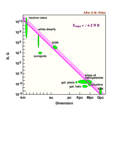
Figure 2: Requirements for acceleration of charged nuclei at astrophysical objects as spelled out by A.M. Hillas (see text).

The reader should note that currently the acceleration of charged nuclei at supernova remnants is mostly a theoretical prediction. Supernova remnants have higher matter density than interstellar space and one expects that the accelerated nuclei would interact with the matter and generate high energy $\gamma$-rays.

Although Cherenkov gamma ray telescopes have observed supernova remnants with TeV $\gamma$-ray emission, there is no proof that TeV and higher energy $\gamma$-rays are generated in hadronic interactions. On the other hand, multi-wavelength observations show the existence of very strong shocks in supernova remnants with TeV $\gamma$-ray emission.

We should then turn to extragalactic objects for acceleration to energies exceeding 10²⁰ eV. The scale for such acceleration was set up by Hillas [9] from basic dimensional arguments. The first requirement for acceleration of charged nuclei in any type of object is that the magnetic field of the object contains the accelerated nucleus within the object itself. One can thus calculate a maximum theoretical acceleration energy, that does not include and efficiency factor, as $E_{max}\leq\gamma eZBR\;,$ where $\gamma$ is the Lorentz factor of the shock matter, $Z$ is the charge of the nucleus, $B$ is the magnetic field value. and $R$ is the linear dimension of the object.

Figure 2, which is a redrawn version of the original figure of Hillas, shows what are the requirements for acceleration to more than 10²⁰ eV. The lower edge of the shaded area shows the minimum magnetic field value for acceleration of iron nuclei as a function of the dimension of the astrophysical object. The upper edge is for acceleration of protons.

There are very few objects that can, even before an account for efficiency, reach that energy: highly magnetized neutron stars, active galactic nuclei, lobes of giant radiogalaxies, and possibly Gpc size shocks from structure formation. Other potential acceleration sites, gamma ray bursts, are not included in the figure because of the time dependence of magnetic field and dimension.

2.1 Possible Astrophysical Sources of UHECR

In this subsection we give a brief description of some of the models for UHECR acceleration at specific astrophysical objects. For a more complete discussion one should consult a review paper on the astrophysical origin of UHECR [10], that contains an exhaustive list of references to particular models.

• Pulsars: Young magnetized neutron stars with surface magnetic fields of 10¹³ Gauss can accelerate charged iron nuclei up to energies of 10²⁰ eV [11]. The acceleration process is magnetohydrodynamic, rather than stochastic as it is at astrophysical shocks. The acceleration spectrum is very flat proportional to 1/$E$. It is possible that a large fraction of the observed UHECR are accelerated in our own Galaxy. There are also models for UHECR acceleration at magnetars, neutron stars with surface magnetic fields up to 10¹⁵ Gauss.

• Active Galactic Nuclei: As acceleration site of UHECR jets [12] of AGN have the advantage that acceleration on the jet frame could have maximum energy smaller than these of the observed UHECR by 1/$\Gamma$, the Lorentz factor of the jet. The main problem with such models is most probably the adiabatic deceleration of the particles when the jet velocity starts slowing down.

• Gamma Ray Bursts: GRBs are obviously the most energetic processes that we know about. The jet Lorentz factors needed to model the GRB emission are of order 100 to 1000. These models became popular with the realization that the arrival directions of the two most energetic cosmic rays coincide with the error circles of two powerful GRB. Different theories put the acceleration site at the inner [13] or the outer [14] GRB shock. To explain the observed UHECRs with GRBs one needs fairly high current GRB activity, while most of the GRB with determined redshifts are at $Z\;>$ 1.

• Giant Radio Galaxies: One of the first concrete model for UHECR acceleration is that of Rachen&Biermann, that dealt with acceleration at FR II galaxies [15]. Cosmic rays are accelerated at the ‘red spots’, the termination shocks of the jets that extend at more than 100 Kpc. The magnetic fields inside the red spots seem to be sufficient for acceleration up to 10²⁰ eV, and the fact that these shocks are already inside the extragalactic space and there will be no adiabatic deceleration. Possible cosmologically nearby objects include Cen A (distance of 5 Mpc) and M87 in the Virgo cluster (distance of 18 Mpc).

• Quiet Black holes: These are very massive quiet black holes, remnants of quasars, as acceleration sites [16]. Such remnants could be located as close as 50 Mpc from our Galaxy. These objects are not active at radio frequencies, but, if massive enough, could do the job. Acceleration to 10²⁰ requires a mass of 10⁹ M_⊙.

• Colliding Galaxies: These systems are attractive with the numerous shocks and magnetic fields of order 20 $\mu$G that have been observed in them [17]. The sizes of the colliding galaxies are very different and with the observed high fields may exceed the gyroradius of the accelerated cosmic ray.

• Clusters of Galaxies: Magnetic fields of order several $\mu$G have been observed at lengthscales of 500 Kpc. Acceleration to almost 10²⁰ eV is possible, but most of the lower energy cosmic rays will be contained in the cluster forever and only the highest energy particles will be able to escape [18].

• Gpc scale shocks from structure formation: A combination of Gpc scales with 1 nG magnetic field satisfies the Hillas criterion, however the acceleration at such shocks could be much too slow, and subject to large energy loss.

2.2 Top-Down Scenarios

Since it became obvious that the astrophysical acceleration up to 10²⁰ eV and beyond is very difficult and unlikely, a large number of particle physics scenarios were discussed as explanations of the origin of UHECR. To distinguish them from the acceleration (bottom-up) processes they were called top-down. The basic idea is that very massive (GUT scale) $X$ particles decay and the resulting fragmentation process downgrades the energy to generate the observed UHECR. Since the observed cosmic rays have energies orders of magnitude lower than the $X$ particle mass, there are no problems with achieving the necessary energy scale. The energy content of UHECR is not very high, and the $X$ particles do not have to be a large fraction of the dark matter. There is a large number of topological defect models which are extensively reviewed in Ref. [19].

There are two distinct branches of such theories. One of them involves the emission of $X$ particles by topological defects. This type of models follows the early work of C.T. Hill [20] who described the emission from annihilating monopole/antimonopole pair, which forms a metastable monopolonium. The emission of massive $X$ particles is possible by superconducting cosmic string loops as well as from cusp evaporation in normal cosmic strings and from intersecting cosmic strings. The $X$ particles then decay in quarks and leptons. The quarks hadronize in baryons and mesons, that decay themselves along their decay chains. The end result is a number of nucleons, and much greater (about a factor of 30 in different hadronization models) and approximately equal number of $\gamma$-rays and neutrinos.

A monopole is about 40 heavier than a $X$ particle, so every monolonium can emit 80 of them. Using that number one can estimate the number of annihilations that can provide the measured UHECR flux, which turns out to be less than 1 per year per volume such as that of the Galaxy. Another possibility is the emission of $X$ particles from cosmic necklaces - a closed loop of cosmic string including monopoles. This particular type of topological defect has been extensively studied [21].

The other option is that the $X$ particles themselves are remnants of the early Universe. Their lifetime should be very long, maybe longer than the age of the Universe [22]. They could also be a significant part of the cold dark matter. Being superheavy, these particle would be gravitationally attracted to the Galaxy and to the local supercluster, where their density could well exceed the average density in the Universe.

There are two main differences between bottom-up and top-down models of UHECR origin. The astrophysical acceleration generates charged nuclei, while the top-down models generate mostly neutrinos and $\gamma$-rays plus a relatively small number of protons. The energy spectrum of the cosmic rays that are generated in the decay of $X$ particles is relatively flat, close to a power law spectrum of index $\alpha$=1.5. The standard acceleration energy spectrum has index equal to or exceeding 2.

2.3 Hybrid Models

There also models that are hybrid, they include elements of both groups. The most successful of those is the Z-burst model [23, 24]. The idea is that somewhere in the Universe neutrinos of ultrahigh energy are generated. These neutrinos annihilate with cosmological neutrinos in our neighborhood and generate $Z_{0}$ bosons which decay and generate a local flux of nucleons, pions, photons and neutrinos. The resonant energy for $Z_{0}$ production is 4$\times$10²¹ eV/$m_{\nu}$(eV), where $m_{\nu}$ is the mass of the cosmological neutrinos. The higher the mass of the cosmological neutrinos is, the lower the resonance energy requirement. In addition the cosmological neutrinos are gravitationally attracted to concentrations of matter and their density increases in our cosmological neighborhood. If the neutrino masses are low, of order of the mass differences derived from neutrino oscillations, the energy of the high energy neutrinos should increase.

3 PROPAGATION OF UHECR

Particles of energy 10²⁰ eV can interact on almost any target. The most common, and better known, target is MBR. It fills the whole Universe and its number density of 400 cm^-3 is large. The interactions on the radio and infrared backgrounds (IRB) are also important. Let us have a look at the main processes that cause energy loss of nuclei and gamma rays.

3.1 Energy Loss Processes

The main energy loss process for protons is the photoproduction on astrophysical photon fields $p\gamma\rightarrow p+n\pi$. The minimum center of mass energy for photoproduction is $\sqrt{s_{thr}}=m_{p}+m_{\pi^{0}}\;\sim$ 1.08 GeV. Since $s=m_{p}^{2}+2(1-\cos{\theta})E_{p}\epsilon$ (where $\theta$ is the angle between the two particles) one can estimate the proton threshold energy for photoproduction on the MBR (average energy $\epsilon\;=$ 6.3$\times$10^-4 eV). For $\cos{\theta}$ = 0 the proton threshold energy is $E_{thr}$ = 2.3$\times$10²⁰ eV. Because there are head to head collisions and because the tail of the MBR energy spectrum continues to higher energy, the intersection cross section is non zero above proton energy of 3$\times$10¹⁹ eV.

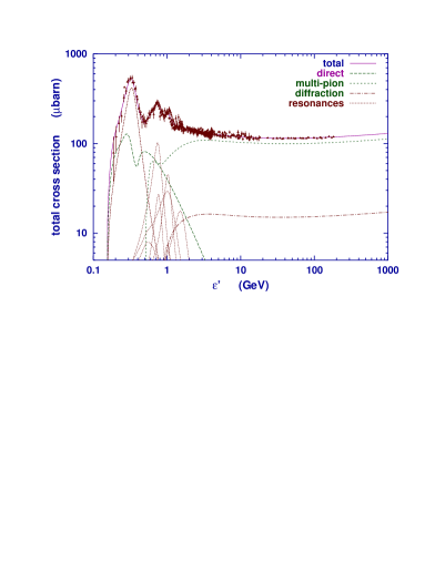
Figure 3: Photoproduction cross section as a function of the photon energy for stationary proton targets.

The photoproduction cross section is very well studied in accelerator experiments and is known in detail. Figure 3 shows the photoproduction cross section in the mirror system [25], as a function of the photon energy for stationary protons, i.e. as it is measured in accelerators. At threshold the most important process is the $\Delta^{+}$ production where the cross section reaches a peak exceeding 500 $\mu$b. It is followed by a complicated range that includes the higher mass resonances and comes down to about 100 $\mu$b. After that one observes an increase that makes the photoproduction cross section parallel to the $pp$ inelastic cross section. The neutron photoproduction cross section is nearly identical.

Another important parameter is the proton inelasticity $k_{inel}$, the fraction of its energy that a proton loses in one interaction. This quantity is energy dependent. At threshold protons lose about 18% on their energy. With increase of the CM energy this fractional energy loss increases to reach asymptotically 50%.

The proton pair production $p\gamma\rightarrow e^{+}e^{-}$ is the same process that all charged particles suffer in nuclear fields. The cross section is high, but the proton energy loss is of order $m_{e}/m_{p}$ $\simeq$ 4$\times$10^-4E. Figure 4 shows the energy loss length $L_{loss}=\lambda/k_{inel}$ (the ratio of the interaction length to the inelasticity coefficient) of protons in interactions in the microwave and infrared backgrounds.

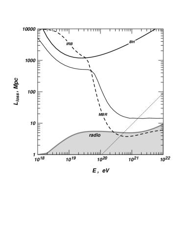
Figure 4: Energy loss length of protons in interactions in MBR and IRB. The shaded area shows the $\gamma\gamma$ interaction length.

The dashed line shows the proton interaction length and one can see the increase of $k_{inel}$ in the ratio of the interaction length to energy loss length. The contribution of the pair production is shown with a thin line. The energy loss length never exceeds 4,000 Mpc, which is the adiabatic energy loss due to the expansion of the Universe for $H_{0}$ = 75 km/s/Mpc. The dotted line shows the neutron decay length. Neutrons of energy less than about 3$\times$10²⁰ eV always decay and only higher energy neutrons interact.

The pair production process deserves more attention since it will become important soon. Figure 5 shows the positron spectra produced in pair production interactions of protons with fixed energy. Next to the proton energy the figure indicates the inelasticity coefficients in these interactions.

Figure 5: Energy distribution of positrons generated in pair production interactions of protons of fixed energy in the MBR.

The pair production cross section grows with the proton energy while the inelasticity coefficient decreases. The combination of both these parameters generates the energy loss length that has a minimum at about 2$\times$10¹⁹ eV.

Heavier nuclei lose energy to a different process - photodisintegration, loss of nucleons mostly at the giant dipole resonance [26]. Since the relevant energy in the nuclear frame is of order 20 MeV, the process starts at lower energy. The resulting nuclear fragment may not be stable. It then decays and speeds up the energy loss of the whole nucleus. Ultra high energy heavy nuclei, where the energy per nucleon is higher than photoproduction, have also loss on photoproduction. The energy loss length for He nuclei in photodisintegration is as low as 10 Mpc at energy of 10²⁰ eV. Heavier nuclei reach that distance at higher total energy. Figure 6 shows the energy loss time of heavy nuclei - 10¹⁴ s equals approximately 1 Mpc.

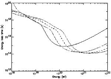
Figure 6: Energy loss length of heavy nuclei (He, O, Si, Fe from left to right in MBR [27].

UHE gamma rays also interact on the microwave background. The main process is $\gamma\gamma\rightarrow e^{+}e^{-}$. This is a resonant process and for interactions in the MBR the minimum interaction length is achieved at 10¹⁵ eV. The interaction length in MBR decreases at higher $\gamma$-ray energy and would be about a 50 Mpc at 10²⁰ eV if not for the radio background. The radio background does exist but its number density is not well known. Figure 4 shows the interaction length for this process in the MBR and the radio background as a shaded area.

The fate of the electrons produced in a $\gamma\gamma$ collision depends on the strength of the magnetic fields in which UHE electrons lose energy very fast. The photon energy is than quickly downgraded and the $\gamma\gamma$ interaction length becomes very close to the gamma ray energy loss length. In the case of very low magnetic fields (0.01 nG) the synchrotron energy loss is low (it is proportional to $E_{e}^{2}B^{2}$) and then inverse Compton scattering (with a cross section very similar to this of $\gamma\gamma$) and cascading is possible. The energy loss length of the gamma rays would be higher in such a case.

The general conclusion from this analysis of the energy loss of protons and gamma rays in their propagation through the Universe is these UHE particles can not survive at distances of more than few tens of Mpc and sources of the detected cosmic rays have to be located in our cosmological neighborhood. Every small increase of the distance between the source and the observer would require increase of the maximum energy at acceleration (or other production mechanism) and will affect significantly the energy requirement for the UHECR sources.

3.2 Modification of the Proton Spectrum in Propagation. Numerical Derivation
of the GZK Effect.

Figure 7 shows the evolution of the spectrum of protons because of energy loss during propagation at different redshifts. The thick solid lines shows the spectrum injected in intergalactic space by the source, which in this exercise is

$$\frac{dN}{dE}\,=\,A\times E^{-2}/\exp({E/10^{21.5}}{\rm eV})\;.$$

After propagation on 10 Mpc (z = 0.0025) some of the highest energy protons are missing. This trend continues with distance and at about 40 Mpc another trend appears - the flux of protons of energy just below 10²⁰ eV is above the injected one. This is the beginning of the formation of a pile-up in the range where the photoproduction cross section starts decreasing. Higher energy particles that are downgraded in this region lose energy less frequently and a pile-up is developed.

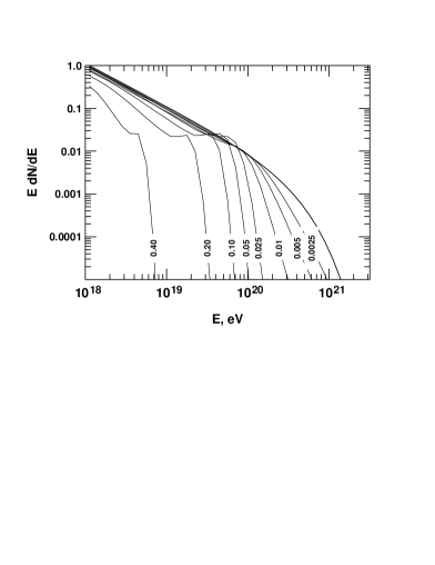
Figure 7: Evolution of the cosmic ray spectrum in propagation through different redshifts.

The pile-up is better visible in the spectra of protons propagated at larger distances. One should remark that the size of the pile-up depends very strongly on the shape of the injected spectrum. If it had a spectral index of 3 instead of 2 the size of the pile-up would have been barely visible as the number of high energy particles decreased by a factor of 10.

When the propagation distance exceeds redshift of 0.4 there are no more particles of energy above 10¹⁹ eV independently of the maximum acceleration energy. All these particles have lost energy in photoproduction, pair production and adiabatic losses. From there on most of the losses are adiabatic.

In order to obtain the proton spectrum created by homogeneously and isotropically distributed cosmic ray sources filling the whole Universe one has to integrate a set of such (propagated) spectra in redshift using the cosmological evolution of the cosmic ray sources, which is usually assumed to be the same as that of the star forming regions (SFR) $\eta(z)\;=\;\eta(0)(1+z)^{n}$ with $n$ = 3, or 4 up to the epoch of maximum activity $z_{max}$ and then either constant or declining at higher redshift. High redshifts do not contribute anything to UHECR ($z$ = 0.4 corresponds to a propagation distance of 1.6 Gpc for $H_{0}$ = 75 km/s/Mpc). After accounting for the increased source activity the size of the pile-ups has a slight increase.

Apart from the pile-up, there is also a dip at about 10¹⁹ eV which is due to the energy loss on pair production. It is also preceded by a small pile-up at the transition from adiabatic to pair production loss. This feature was first pointed at by Berezinsky&Grigorieva [28].

The GZK cutoff, the pile-up and the pair production dip characterize the energy spectrum of extragalactic protons under the assumptions of injection spectrum shape, cosmic ray luminosity, cosmological evolution and isotropic distribution of the cosmic ray sources in the Universe.

3.3 Modification of the Gamma Ray Spectra from top-down models.

Because of the strong influence of the radio background and of the cosmic magnetic fields the modification of the spectrum of gamma rays in a top-down scenario is much more difficult to calculate exactly. There are, however, many general features that are common in any of the calculations. Figure 8 shows the gamma ray spectrum emitted in a top-down scenario with $m_{X}$ = 10¹⁴ GeV [29]. The spectra of $\gamma$-rays and electrons from the $X$ decay chain are indicated with different line types.

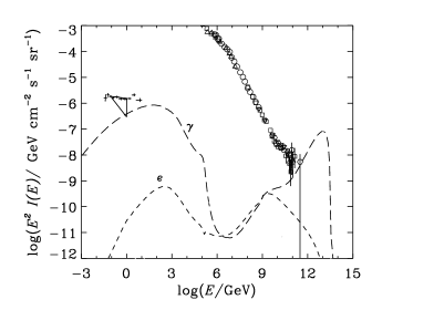
Figure 8: Evolution of the energy spectra of electrons and $\gamma$-rays injected in a top-down scenario with $X$ particle mass of 10¹⁴ GeV.

The typical gamma ray energy spectrum in top-down models is E^-3/2. We shall start the discussion from the highest energy and follow the energy dissipation in propagation. The highest energy gamma rays have not suffered significant losses. At slightly lower energy, though, the $\gamma\gamma$ cross section grows and the energy loss increases. One can see the dip at about 10^10-11 GeV which is caused by the radio background. The magnetic field is assumed sufficiently high that all electrons above 10⁹ GeV immediately lose energy in synchrotron radiation. The minimum ratio of the gamma-ray to cosmic ray flux is reached at about 10¹⁵ eV, where the minimum of the interaction length in the MBR is, after which there is some recovery. There is another absorption feature from interactions on the infrared background. The gamma ray peak in the GeV region consists mostly of synchrotron photons. Isotropic GeV gamma rays, that have been measured, can be used to restrict top-down models in some assumptions for the magnetic field strength.

3.4 UHECR Propagation and Magnetic Fields

The possible existence of non negligible extragalactic magnetic fields would modify the propagation of the UHE cosmic rays independently of their nature and origin. There is little observational data on these fields. The estimate of the average strength of these fields in the Universe is 10^-9 Gauss (1 nG) [30]. On the other hand $\mu$G fields have been observed in clusters of galaxies, and in a bridge between two parts of the Coma cluster.

Even fields with nG strength would affect the propagation of UHE cosmic rays. If UHECR are protons or heavier nuclei they would scatter of these fields. This scattering would lead to deviations from the source direction and to an increase of the pathlength from the source to the observer. It would make the source directions less obvious and would create a magnetic horizon [31] for extragalactic protons of energy below 10¹⁹ eV as their propagation time from the source to the observer would start exceeding Hubble time. When the horizon is achieved the cosmic ray spectrum appears flatter than it actually is.

Figure 9: Distance from the source that contains more than 50% of the emitted protons.

If regular magnetic fields of strength exceeding 10 nG were present on 10 Mpc coherence length they would lead to significant biases in the propagated spectra [32] in a function of the relative geometry of the field, source and observer. 10¹⁹ eV particles would gyrate around the magnetic field lines and thus appear coming from a wide range of directions. The flux of such particles would be much higher than at injection. Only particles of energy above 10²⁰ eV would be able to propagate through the magnetic field lines.

Ultrahigh energy protons are also affected in propagation by the galactic magnetic fields - they scatter and acquire an angle with their direction outside of the Galaxy. That angle depends on the UHECR rigidity and direction. The largest angle should be when the proton has to propagate close to the galactic center and galactic bulge region where the fields, although not exactly known, are the highest. Excluding the galactic center vicinity, the average deflection angle for 10²⁰ eV protons is between 3.1^o and 4.5^o in different galactic magnetic field models [33].

3.5 Production of Secondary Particles in Propagation

One interesting feature that can be used for testing of the type and distribution of UHECR sources is the production of secondary particles in propagation. The energy loss of the primary protons and $\gamma$-rays is converted to secondary gamma rays and neutrinos (in the case of primary nuclei). Gamma rays are generated in nucleon photoproduction interactions and in BH pair production processes as well as in $\gamma\gamma$ collisions.In the case of isotropic and homogeneous source distribution the gamma ray energy is degraded and eventually converted to MeV/GeV diffuse isotropic flux. The value of this flux could be used to restrict the amount of energy in UHECR [34, 29]. Some cosmologically nearby sources may still create a halo in the source direction of high energy gamma rays that could be detected by the sensitive contemporary TeV gamma ray telescopes.

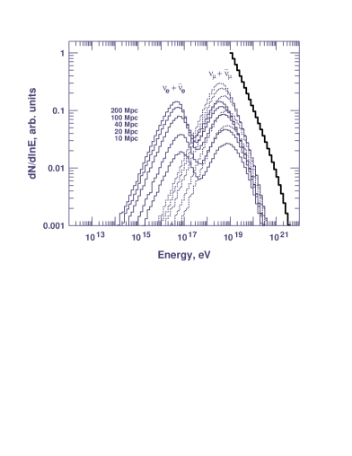
Figure 10: Production of neutrinos from cosmic ray proton propagation on different distances from 10 to 200 Mpc

Most interesting are the cosmogenic neutrinos, that were first proposed by Berezinsky & Zatsepin [35] and have been since calculated many times, most recently in Ref. [36]. Every charged pion produced in a photoproduction interaction generates three neutrinos through its decay chain.

The spectrum of cosmogenic neutrinos depends on the UHECR spectrum, the UHECR source distribution and very strongly on the cosmological evolution of the UHECR sources [37]. The sensitivity to the cosmological evolution of the sources is very high because of the lack of energy loss (except for adiabatic loss) of the generated neutrinos. Figure 10 shows the spectra of neutrinos generated in proton propagation at different distances. In the contemporary Universe muon neutrinos and antineutrinos peak at about 10¹⁸ eV, while electron neutrinos and antineutrinos show a double peaked spectrum. The higher energy peak, coinciding with that of $\nu_{\mu}$ consists mostly of electron neutrinos, while the lower energy one is of $\bar{\nu}_{e}$ from neutron decay. If there is a high fraction of heavy nuclei in the primary UHECR the $\bar{\nu}_{e}$ would dominate the $\nu_{\mu}$ flux since there would be many more neutrons from photodisintegration than photoproduction interactions, which mostly protons and He nuclei would suffer.

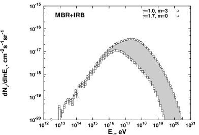
Figure 11: Cosmogenic $\nu_{\mu}+\bar{\nu}_{\mu}$ generated by protons with a flat acceleration spectrum ($\gamma$=1.0) with cosmological evolution and a steep one ($\gamma$=1.7) without evolution.

It is of some importance to note that MBR is not the only target for neutrino production. The second most important one is the isotropic infrared and optical background (IRB). Its number density is, or course, much lower, but lower energy protons can interact in it and even in the case of flat acceleration spectra the number of interacting protons to a large extent compensates for the lower photon target density.

Fig. 11 shows the spectra of $\nu_{\mu}$+$\bar{\nu}_{\mu}$ generated by a flat ($\gamma$=1.0) and steep ($\gamma$=1.7) UHECR acceleration spectra. In the case we are lucky enough to detect cosmogenic neutrinos with the neutrino telescopes under construction and design they could help a lot in limiting the models for the origin of the ultrahigh energy cosmic rays.

4 Experimental data

At this meeting we saw the first set of experimental data with very good statistics observed by the Auger Collaboration. Auger reported the data from an exposure of more than 5,165 km².ster.yr obtained during the construction of the array. This exceeds the exposure of the previous biggest array, Agasa [38], by about a factor of three. The exposure of the HiRes detector is energy dependent as the fluorescent light of higher energy showers can be detected from larger distances. The Auger air shower array consists of 1,600 water tanks of area 10 m² in which the charged shower particles and the converted $\gamma$-rays produce Cherenkov light. Tanks are viewed with 3 photomultipliers. The water tanks have the advantage to have significant effective area for highly inclined showers.

4.1 Cosmic ray spectrum

Auger reported three energy spectra obtained in different manner: one from the surface array normalized to the fluorescent telescopes measurement [39], another from hybrid array, i.e. from showers observed both by the ground array and by the fluorescent detectors [40], and a third one coming from showers arriving at zenith angles exceeding 60^∘ [41]. All three spectra agree with each other within the statistical uncertainties. There is only two events of energy above 10²⁰ eV in this set. The presented spectra thus support the conclusion of HiRes [42, 43] that the cosmic ray spectrum does not continue above 10²⁰ eV with the same $\sim$E^-2.7 spectral index as the Agasa experiment found. There is obviously a steepening of the spectrum which may be consistent with a GZK feature.

There are good reasons to trust the spectrum measurements of the Auger collaboration. The analysis only includes well contained showers by the requirement that the highest hit detector is surrounded by six active detectors. This requirement also guarantees that there is enough information for a good shower analysis. Another requirement is the reconstructed shower core position is inside the 3,000 km² array. For this reason the exposure of Auger is very well known. Only events with reconstructed energy above 3$\times$10¹⁸ eV, where the efficiency is 100%, are included. The uncertainty on the energy estimate is quoted to be 22% - most of it due to fluorescent efficiency.

Figure 12: Comparison of the detailed spectral shapes reported by the Auger Collaboration (surface detector and hybrid events) and by HiRes 1 and 2 in monocular mode.

The overall normalization of the spectrum is somewhat lower than that of HiRes. It also seems to have slightly different shape: the dip in the spectrum above 10¹⁹ eV (seen mostly in the hybrid data set appears deeper and the recovery faster as shown in Fig. 12. The depletion of high energy showers is not that steep and starts a bit earlier. Note that the slopes presented in Fig. 12 are not the same as presented by Auger at the meeting [44] - my fits are probably not as careful as those of the group. As small these differences are, they currently affect the comparison with the UHECR acceleration and propagation models and the derivation of the end of the galactic cosmic ray spectrum (see the talk of Venya Berezinsky in this volume). The solution of these questions will not be made before we have a very good measurement of the UHECR chemical composition.

4.2 UHECR composition

Auger also presented data on the average depth of shower maximum ($X_{max}$) as a function of the shower energy [45]. The average $X_{max}$ is the measure of the cosmic ray chemical composition that could be made by fluorescent detectors. Hybrid events are used in this data set because even one surface detector triggered in coincidence with the fluorescent trigger vastly improves the shower reconstruction. Fig. 13 compares the measurements of HiRes, HiRes Prototype/MIA and Auger, converted to $\langle lnA\rangle$ using the Sibyll2.1 hadronic interaction model. The use of other models would change the derived values, i.e. move the experimental points to lower $\langle lnA\rangle$ values for models having shallower $X_{max}$.

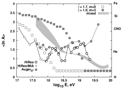
Figure 13: The data of HiRes/MIA, HiRes and Auger are compared to the predictions of three models of UHECR acceleration and propagation.

The two sets of squares and the shaded area plot roughly the $\langle lnA\rangle$ values that come from three types of models: the empty squares correspond to the model of Berezinsky et al [46, 47], full ones correspond to the model of Bahcall & Waxman [48] and the shaded area corresponds to the mixed primary composition model [49, 50]. At very high energy in Fig. 13 I have assumed a standard H + He composition in a ratio of 9:1.

The model of Berezinsky et al is that all cosmic rays above 10¹⁸ eV are of extragalactic origin, and are mostly protons. The acceleration (injection) spectrum is steep with a slope of 1.7. The dip is due to pair production losses. The shape of the spectrum below the dip is determined by the transition to purely adiabatic energy loss. There is no need for a strong cosmological evolution of the cosmic ray sources. The maximum amount of He and heavier nuclei is about 15%. Bahcall & Waxman assume that the dip is where the flat extragalactic UHECR flux ($\gamma$=1) intersects the flux of galactic cosmic rays. A similar model was also proposed by Wibig & Wolfendale [51] with slightly different parameters. The flat acceleration spectrum models require strong cosmological evolution $(1+z)^{3-4}$ to be able to fit the experimental data. Since the extragalactic cosmic rays are mostly H the composition becomes very light after the transition. Obviously in the Berezinsky et al model there is no need of galactic cosmic rays of energy above 10¹⁸ eV, while in the other models the Galaxy has to accelerate particles to energy higher by an order of magnitude.

Mixed UHECR composition model assumes that these particles leave their sources with a composition similar to those of GeV galactic cosmic rays. The composition changes in propagation and above 10^19.5 eV the composition also becomes very light. The injection spectrum is relatively flat ($\gamma$=1.2-1.3). Since the spectrum at Earth depends on the primary composition as well as on the acceleration spectrum it is possible to fit the observations in different ways. The current experimental data on the cosmic ray composition do not seem to support any of the models.

There is, however, a problem in our understanding of the shower development in the atmosphere. If Auger surface detector data were analyzed using existing shower simulations (not normalized to the fluorescent detector) the energy estimate would on average go up by 20-25% and the composition would appear heavier [52]. The only current hadronic interaction model that predicts similar $X_{max}$ and high surface (muon) density is EPOS [53], which is not yet well studied.

For this reason the solution of the problems of the highest energy cosmic rays will have to wait. The differences in the Auger energy estimates by the surface and fluorescent detectors is very similar to the current differences between the AGASA and HiRes spectra after the energy estimate of AGASA has come down by 10-15% with the use of the contemporary hadronic interaction model [54]. The hybrid detection of Auger and the Telescope Array, as well as the theoretical work, will lead us to the solution in the next several years.

One of these problems is almost solved: many experiments and currently Auger [55] have set strict limits on the fraction of gamma-rays in the UHECR flux. For showers above 10¹⁹ eV the limit of Auger is 2%. At higher energy the limits are not that strict because of limited statistics. A general conclusion can be drawn from these limits that UHECR are not the result of top-down models and are due to acceleration in powerful astrophysical objects.

4.3 Arrival directions of UHECR

The question then is which these objects are. The AGASA experiment [56] has seen clustering of the highest energy events, i.e. several groups of two events and one of three events that come from similar directions smaller than the angular resolution of the array. HiRes did not observe that type of clustering. Auger [57] does not confirm the clustering either, although there is still some possibility that some degree of clustering (2% probability for isotropic distribution) exists among the highest energy events.

So we are back to that controversial situation where we know that the astrophysical sources of UHECR have to be close to us in cosmological sense but we can not see them. The Auger Collaboration is in the process of an intensive search for anisotropies and correlations with different types of astrophysical objects in their data sample. Since we expect a very strong increase in their statistics even during the next year we hope future data will help resolving this situation.

5 Summary

The cosmic ray spectrum steepens at the approach of 10²⁰ eV according to the HiRes and the new Auger data. Is this steepening the long expected GZK feature or is it of a different origin? An example for a different origin could be the inability of the sources to accelerate cosmic rays of energy higher than 5$\times$10¹⁹ eV. Solving this would require higher statistics than is currently available.

The current statistics is, however, enough to establish the fact that 1-2$\times$10¹⁹ eV cosmic rays are not $\gamma$-rays. This fact supports the acceleration bottom-up scenarios for cosmic ray production. At the higher energies more statistics is needed to set limits of a higher quality. Thus it is still possible (although not likely) that the highest energy events could result from top-down models.

It is not currently obvious what the cosmic ray nuclear composition is in the energy range above 10¹⁸ eV. The Auger data points at a composition that is somewhat heavier than the one derived by the HiRes experiment. Differences are not statically significant yet. Composition measurements are hurt by the insufficient understanding of the shower development. Current hadronic interaction models should improve after comparisons with the Large Hadronic Collider (LHC) data that will become available soon.

We still can not see the UHECR sources. Studies of anisotropy, in addition of revealing the UHECR sources, are complimentary to the composition studies. If these particles were heavy nuclei they would scatter stronger in the magnetic fields and show smaller correlation with their sources. Protons would more or less point at their sources. The identification of the UHECR sources would also contribute to our knowledge of magnetic fields in the Galaxy and the Universe.

We are now in a period when the UHECR statistics is increasing very fast and will help the solution of the problems listed above. In addition to Auger and TA the work on a satellite based UHECR Observatory continues. While the previous two projects, EUSO [58] and OWL [59] barely exist anymore, the Japanese JEM/EUSO project, that is to be installed at the Japanese module of the International Space Station is doing well and may be launched in 2013. Such an experiment would increase the statistics by another factor of 10 over the surface arrays.

Finally, the neutrino astronomy projects are also in the process of fast development. Auger is looking for horizontal air showers initiated by neutrinos, the construction of IceCube [60] is going extremely well, and the radio detection of UHE neutrinos is also moving forward. The possible detection of cosmogenic neutrinos will help the solution of the UHECR origin when compared to the direct observations.

6 Acknowledgments

The author has benefited from discussions with V.S. Berezinsky, P. Blasi, D. DeMarco, T.K. Gaisser, D. Seckel, and A.A. Watson. D. Allard helped me with understanding of the heavy nuclei model of UHECR. This work is supported in part by NASA APT grant NNG04GK86G.

References

- [1] J. Linsley, Phys. Rev. Lett., 10, 146 (1963)
- [2] G. Cocconi, Nuovo Cimento, 3, 1422 (1956)
- [3] K. Greisen, Phys. Rev. Lett. 16, 748 (1966)
- [4] G.T. Zatsepin & V.A. Kuzmin, JETP Lett. 4 78 (1966).
- [5] http://www.auger.org
- [6] http://www-ta. icrr.u-tokyo.ac.jp
- [7] D.J. Bird et al., Phys. Rev. Lett., 71, 3401 (1993)
- [8] H.J. Völk & P.L. Biermann, ApJ, 333 L65 (1988)
- [9] A.M. Hillas, Ann. Rev. Astron. Astrophys., 22, 425 (1984)
- [10] D.F. Torres & L.A. Anchordoqui, Rep. Prog. Phys., 67, 1663 (2004)
- [11] P. Blasi, R.I. Epstein & A.V. Olinto, Ap.J., 533, L33 (2000)
- [12] F. Halzen & E. Zas, Ap. J., 488, 607 (1997)
- [13] E. Waxman, Ap. J., 452 1 (1995)
- [14] M. Vietri, Ap. J., 453, 883 (1995)
- [15] J.P. Rachen & P.L. Biermann, A&A, 272, 161 (1993)
- [16] E. Boldt & P. Ghosh, MNRAS, 307, 491 (1999)
- [17] C.J. Cesarsky, Nucl. Phys. B (Proc. Suppl.), 28, 51 (1992)
- [18] H. Kang, D. Ryu & T.W. Jones, Ap. J., 456, 422 (1998).
- [19] P. Bhattacharjee & G. Sigl, Phys. Reports, 327, 109 (2000)
- [20] C.T. Hill, Nucl. Phys., b224, 469 (1983)
- [21] V.S. Berezinsky& A. Vilenkin, Phys. Rev. Lett., 79, 5202 (1997)
- [22] V.S. Berezinsky, M. Kahelriess & A. Vilenkin, Phys. Rev. Lett., 79, 4302 (1997)
- [23] T.J. Weiler, Astropart. Phys., 11, 303 (1999)
- [24] D. Fargion, B. Mele & A. Salis, Ap. J., 517, 725 (1999)
- [25] A. Mücke et al, Comp. Phys. Comm., 124, 290 (2000)
- [26] J.L. Puget, F.W. Stecker & J.H. Bredekamp, Ap. J., 205, 538 (1976)
- [27] G. Bertone et al, Phys. Rev. D66:103003 (2002)
- [28] V.S. Berezinsky & S.I. Grigorieva, A&A, 199, 1 (1988)
- [29] R.J. Protheroe and T. Stanev, Phys. Rev. Letters, 77, 3708 (1996)
- [30] P.P. Kronberg, Rep. Progr. Phys., 57, 325 (1994)
- [31] T. Stanev et al, Phys. Rev. D62:093005 (2001)
- [32] T. Stanev, D. Seckel & R. Engel, Phys. Rev. D, 68:103004 (2003)
- [33] T. Stanev, ApJ 478:290 (1997)
- [34] V.S. Berezinsky & A.Yu. Smirnov, Astrophys & Space Sci, 32, 461 (1975)
- [35] V.S. Berezinsky & G.T. Zatsepin, Phys. Lett. 28b, 423 (1969); Sov. J. Nucl. Phys. 11, 111 (1970).
- [36] R. Engel, D. Seckel & T. Stanev, Phys. Rev. D64:09310 (2001)
- [37] D. Seckel & T. Stanev, Phys. Rev. Lett., 95:141101 (2005)
- [38] M. Takeda et al., Phys. Rev. Lett., 81, 1163 (1998); for updates see http://www-akeno.icrr.u-tokio.ac.jp
- [39] M. Roth for the Pierre Auger Collaboration, ArXiv:0706.2096 (2007)
- [40] L. Perrone for the Pierre Auger Collaboration, ArXiv:0706.2643 (2007)
- [41] P. Facal for the Pierre Auger Collaboration, ArXiv:0706.4322 (2007)
- [42] R.U. Abbasi et al. (HiRes Collaboration), Phys. Rev. Lett., 92: 151101 (2004)
- [43] T. Abu-Zayyad et al.(HiRes Collaboration), Astropart. Phys., 23, 157 (2005)
- [44] T. Yamamoto for the Pierre Auger Collaboration, ArXiv:0707.2638 (2007)
- [45] M. Unger for the Pierre Auger Collaboration, ArXiv:0706.1495 (2007)
- [46] V.S. Berezinsky, A.Z. Gazizov and S.I. Grigorieva, Phys. Lett. B612:147 (2005)
- [47] R. Aloisio et al., Astropart. Phys. 27:76 (2007)
- [48] J.N. Bahcall & E. Waxman, Phys. Lett. B556:1-6 (2003)
- [49] D. Allard et al., A&A 443:L29 (2005)
- [50] D. Allard et al., Astropart.phys. 27:61 (2007)
- [51] T. Wibig & A.W. Wolfendale, J.Phys. G31:255 (2005)
- [52] R. Engel for the Pierre Auger Collaboration, ArXiv:0706.1921 (2007)
- [53] K. Werner & T. Pierog, AIP Conf. Proc. 928:111-117,2007.
- [54] M. Teshima, talks at Vulcano 2006 and CRIS 2006 workshops.
- [55] M. Healy for the Pierre Auger Collaboration, ArXiv:0710.0025 (2007)
- [56] Y. Uchihori et al., Astropart. Phys., 13, 151 (2000)
- [57] S. Mollerach for the Pierre Auger Collaboration, ArXive:0706.1749 (2007)
- [58] http://www.euso-mission.org
- [59] http://owl.gsfc.nasa.gov
- [60] http://icecube.wisc.edu