Intrinsic channel closing in strong-field single ionization of $\mathbf{\mathrm{H}_{2}}$

Abstract

The ionization of $\mathrm{H}_{2}$ in intense laser pulses is studied by numerical integration of the time-dependent Schrödinger equation for a single-active-electron model including the vibrational motion. The electron kinetic-energy spectra in high-order above-threshold ionization are strongly dependent on the vibrational quantum number of the created ${\mathrm{H}_{2}}^{+}$ ion. For certain vibrational states, the electron yield in the mid-plateau region is strongly enhanced. The effect is attributed to channel closings, which were previously observed in atoms by varying the laser intensity.

Above-threshold ionization (ATI) Agostini et al. (1979); Eberly et al. (1991) of atoms or molecules by intense laser fields stands for the absorption of more photons than needed to overcome the ionization threshold. A simple analysis of classical electron trajectories shows that electrons rescattering once from the core after the initial ionization step attain large final energies up to $10U_{\mathrm{p}}$ Paulus et al. (1994a, b, 1995), while direct (unscattered) electrons have a maximum energy of $2U_{\mathrm{p}}$. Here, $U_{\mathrm{p}}$ denotes the ponderomotive potential. A striking phenomenon arises when high-order ATI is studied with respect to its dependence on laser intensity. For the rescattering plateau between $2U_{\mathrm{p}}$ and $10U_{\mathrm{p}}$, it was found in experiment Hansch et al. (1997); Hertlein et al. (1997) and calculations Muller and Kooiman (1998); Muller (1999); Paulus et al. (2001); Kopold et al. (2002); Popruzhenko et al. (2002); Wassaf et al. (2003); Krajewska et al. (2006), that a slight change in laser intensity can lead to order-of-magnitude changes in yield for groups of peaks within the plateau. Explanations were found in terms of multiphoton resonances with Rydberg states Muller and Kooiman (1998); Muller (1999); Potvliege and Vučić (2006) and within the framework of quantum paths Kopold et al. (2000); Paulus et al. (2001); Kopold et al. (2002). The spectral enhancements can be related to channel closings that occur when the (ponderomotively shifted) lowest ATI peak coincides with an effective threshold Paulus et al. (2001); Kopold et al. (2002).

In the present work, we investigate the role of molecular vibration in ATI channel closings, using the example of the ${\mathrm{H}_{2}}$ molecule. Due to the additional degree of freedom, an additional energy scale is involved in the dynamics. In the case of atoms, channel closings were introduced by scanning through a certain range of laser intensities. We show that for molecules, due to the coupling between electronic and nuclear motion, intrinsic channel closing effects can be observed by comparing the electron-spectra for different vibrational states of the created ${{\mathrm{H}_{2}}^{+}}$ ion, i.e., applying only one laser intensity.

The minimum energy of a free electron in the presence of a laser field with amplitude $F_{0}$ and frequency $\omega$ is equal to the ponderomotive potential (atomic units are used unless stated otherwise) $U_{\mathrm{p}}=F_{0}^{2}/4\omega^{2}$, which is the quiver energy of the free oscillating electron. Therefore, the laser field modifies the ionization threshold. In non-resonant $n$-photon ionization of an atom, the electron carries the final kinetic energy

$$E_{\text{kin}}=n\,\omega-I_{\mathrm{p}}-U_{\mathrm{p}},$$ (1)

with the ionization potential $I_{\mathrm{p}}$ and integer $n$. The minimum number $s$ of photons needed to free a bound electron is therefore defined through $s=\text{ceil}[(I_{\mathrm{p}}+U_{\mathrm{p}})/\omega]$. By scanning through a range of laser intensities and thus varying $U_{\mathrm{p}}$, one can let ATI peaks disappear at the beginning of the spectrum. Such a channel closing causes build-up of electron probability near the core Muller and Kooiman (1998) and therefore leads to significant enhancements of groups of peaks within the rescattering plateau of the ATI spectrum. Note however, that the precise intensities at which this effect occurs deviate from the estimate based on the simple formula above Paulus et al. (2001); Kopold et al. (2002).

Dealing with molecules, due to the coupling of electronic and vibrational motion, energy is also transferred to the nuclei of the system, leading to the occupation of vibrationally excited states. We expect that for a given vibrational state of the created ${{\mathrm{H}_{2}}^{+}}$ ion, Eq. (1) is changed to

$$E_{\text{kin}}=n\,\omega-I_{\mathrm{p}}-U_{\mathrm{p}}-\Delta E^{v},$$ (2)

where $\Delta E^{v}=E^{v}-E^{0}$ is the difference in vibrational energy between the vibrationally excited state $v$ in question and the vibrational ground state. Note that $I_{\mathrm{p}}$ denotes here the adiabatic, not the vertical ionization potential .

Our model of the ${\mathrm{H}_{2}}$ molecule consists of a single active electron, interacting with two protons that are screened by a second (inactive) electron. The electronic motion is restricted to the polarization direction of the laser field. We mention that the effect of moving nuclei in ATI of 1D ${{\mathrm{H}_{2}}^{+}}$ has been studied previously Bandrauk et al. (2003), but not in the context of channel closings. Note that the dynamics of two active electrons coupled to the vibrational motion has been treated earlier within 1D models of ${\mathrm{H}_{2}}$ Kreibich et al. (2001); Saugout et al. (2007), but so far it has not been achieved to calculate ATI spectra within that approach. In the present work, the molecular alignment is perpendicular, i.e., the polarization direction is perpendicular to the nuclear motion. This choice was made to eliminate the dipole coupling between the electronic ground and first excited state of the ${{\mathrm{H}_{2}}^{+}}$ ion and hence allow for high vibrational excitation of the electronic ground state Urbain et al. (2004). This leads to the Hamiltonian

$$\begin{split}\widehat{H}(z,R,t)=&-\frac{1}{2}\biggl{(}\frac{1}{\mu_{\mathrm{n}}}\frac{\mathrm{d}^{2}}{\mathrm{d}R^{2}}+\frac{1}{\mu_{\mathrm{e}}}\frac{\mathrm{d}^{2}}{\mathrm{d}z^{2}}\biggr{)}\\ &\qquad\qquad+V_{\mathrm{n}}(R)+V_{\text{int}}(z,R)+E(t)z,\end{split}$$ (3)

where the operator $E(t)z$ with $E(t)=F(t)F_{0}\sin(\omega t)$ describes the interaction of the electron with the electric field of a linearly polarized laser pulse in length gauge. The quantity $F(t)$ defines the pulse shape and $F_{0}$ is the maximum field amplitude. The electron coordinate and inter-nuclear distance are denoted by $z$ and $R$; $\mu_{\mathrm{e}}$ and $\mu_{\mathrm{n}}$ denote the reduced masses of the active electron and of the two nuclei, respectively. The vibrational motion in the ${{\mathrm{H}_{2}}^{+}}$ ion is incorporated in the model by inserting the exact Born-Oppenheimer ground-state potential of ${{\mathrm{H}_{2}}^{+}}$,

$$V_{\mathrm{n}}(R)=V_{\text{BO}}^{{{\mathrm{H}_{2}}^{+}}}\!(R).$$ (4)

This choice reflects the assumption that the second (inactive) electron stays in the ground state at all times. The active electron interacts with the ${{\mathrm{H}_{2}}^{+}}$ ion via a soft-core potential

$$V_{\text{int}}(z,R)=-\frac{1}{\sqrt{z^{2}+\sigma^{2}(R)}}.$$ (5)

The idea behind this model is that the core, consisting of the proton charges screened by the inactive electron, is treated as one, singly charged object. The values of $\sigma(R)$ are fitted such that the ground-state Born-Oppenheimer potential of the ${\mathrm{H}_{2}}$ model Hamiltonian matches the exact ${\mathrm{H}_{2}}$ Born-Oppenheimer ground-state potential $V_{\text{BO}}^{\mathrm{H}_{2}}\!(R)$ known from the literature Kołos et al. (1985). A similar fitting procedure has been used previously to reproduce the Born-Oppenheimer potential of ${{\mathrm{H}_{2}}^{+}}$ in a 1D model Feuerstein and Thumm (2003). Since our model does not allow excitation of the second electron, we have excluded the Coulomb explosion channel, which has been extensively studied for example in Chelkowski et al. (2007).

The propagation of the time-dependent wave function is based on the split-operator method, along with 2D Fourier transformations to apply the kinetic-energy-dependent operators as simple multiplications in momentum space. The two-dimensional grid ($z$-spacing 0.36 a.u., $R$-spacing 0.05 a.u.) extends in $R$-direction from 0.2 a.u. to 12.95 a.u., in electronic direction from -276.3 a.u. to 276.3 a.u., corresponding to 256 and 1536 grid points, respectively. In the electronic dimension, the grid is further extended up to $\left|z\right|=$ 2522.7 a.u. using a splitting technique Grobe et al. (1999): in this outer region the 2D wave function $\Psi_{\mathrm{out}}(z,R,t)$ is expanded into products states, i.e.,

$$\Psi_{\mathrm{out}}(z,R,t)=\sum_{j}\xi_{j}(z,t)\zeta_{j}(R,t),$$ (6)

where $\xi_{j}(z,t)$ and $\zeta_{j}(R,t)$ are so-called canonical basis states or natural orbitals Löwdin (1955), making a single summation over product states possible. They are obtained as the eigenstates of the one-particle density matrices of the two coordinates $z$ and $R$, respectively, for those portions of the wave function that are transferred to the outer region. The number of expansion terms is chosen to keep at least 99.9% of the total probability. No more than four terms were needed in each expansion. Within the outer region, the interaction potential $V_{\text{int}}(z,R)$ is replaced by the $R$-independent potential $V_{\mathrm{out}}(z)=V_{\mathrm{int}}(z,R=2)$. The coupling between $z$ and $R$ is thus removed in this area, and 1D propagations can be applied separately to the functions $\xi_{j}(z,t)$ and $\zeta_{j}(R,t)$, which allows for large grids. This helps to keep the entire probability on the grid in spite of the vast electron excursions in strong pulses. It also leads to high resolution of the kinetic-energy spectra. In the range of $\left|z\right|=10\ldots 161$ a.u., the interaction is smoothly varied from $V_{\mathrm{int}}$ to $V_{\mathrm{out}}$. This means that unlike Grobe et al. (1999), our calculation does not involve a discontinuity of the Hamiltonian at the boundary between inner and outer grid.

The pulse shape $F(t)$ is chosen such that the temporal pulse integral vanishes. The pulses have a plateau with constant intensity around the middle of the pulse. The leading and trailing edge of the pulses are $\sin^{2}$-shaped ramps. The total pulse length counts five cycles, where 1.5 cycles are used to ramp the pulse on and off, respectively. The plateau therefore extends over two cycles. After the end of the pulse, three empty cycles follow to allow for the continuum electrons to significantly escape from the Coulomb potential of the ${{\mathrm{H}_{2}}^{+}}$ ion before the simulation ends. The laser wavelength is 800 nm so that we have $I_{\mathrm{p}}=10.0~{}\omega$. The system is regarded as ionized for $\left|z\right|>$ 30 a.u. The precise choice of this value is not important since the results shown in this work involve electrons driven at least 500 a.u. from the ion at the end of the simulation.

Projecting the ionized part $\Psi_{\mathrm{ion}}$ (see above) of the final wave function onto the different vibrational states $\chi_{v}$ of ${{\mathrm{H}_{2}}^{+}}$,

$$\phi_{v}(z)=\int\chi_{v}^{\textstyle*}(R)\,\Psi_{\mathrm{ion}}(z,R,t_{\mathrm{end}})\;\mathrm{d}R,$$ (7)

leads to one ATI spectrum for each vibrational state considered. The spectra are calculated via Fourier transformation to $\widetilde{\phi}_{v}(p_{z})$, followed by rescaling of the modulus square $|\widetilde{\phi}_{v}(p_{z})|^{2}$ from momentum to energy. Only the right-going part of the wave function is used in this work.

According to Eq. (2), the ATI peaks within these spectra are shifted by $\Delta E^{v}$. Hence, channel closings can be observed by variation of $v$. Since $\Delta E^{v}$ can easily exceed the photon energy (for the ${{\mathrm{H}_{2}}^{+}}$ ion and $\lambda=800$ nm, $\Delta E^{7}\approx 1.0\,\omega$), the channel closing will always take place, no matter where exactly the first ATI peak is located. The different vibrational levels play the role of the different laser intensities in the atomic case. As soon as the vibrational energy eats up enough energy, we expect that the energy spectrum for the corresponding electrons shows the characteristic channel closing features known from atoms.

In Fig. 1, kinetic-energy spectra

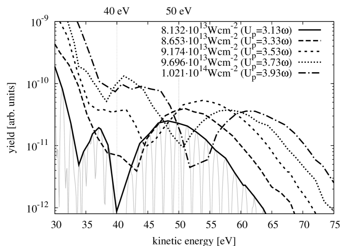
Figure 1: Envelopes of kinetic-energy spectra of (right-going) ATI electrons leaving the ${{\mathrm{H}_{2}}^{+}}$ ion in the $v=4$ vibrationally excited state. The various laser intensities correspond to ponderomotive potentials between $U_{\mathrm{p}}=3.13~{}\omega$ and $U_{\mathrm{p}}=3.93~{}\omega$.

of ATI electrons belonging to ${{\mathrm{H}_{2}}^{+}}$ ions that are produced in the $v=4$ vibrationally excited state are shown. To enhance readability, except for one example only the envelopes are plotted. Since the spectra correspond to a single vibrational state of the ion, an atom-like ATI spectrum arises for each laser intensity, and an atom-like channel closing can be identified. All spectra contain only data from the $z>0$ part of the grid because a slight difference in peak positions between $z<0$ and $z>0$ would lead to blurring of the peaks. The envelope top reaches its highest value for an intensity of $I=9.70\times 10^{13}~{}\mathrm{W}/\mathrm{cm}^{2}$ ($U_{\mathrm{p}}=3.73~{}\omega$) at around $42~{}\mathrm{eV}$. Trying to estimate this intensity from in Eq. (2), the term $\Delta E^{v}$ is kept constant while $U_{\mathrm{p}}$ is scanned through. Using Eq. (2), we find the channel closing ($E_{\mathrm{kin}}=0$) to be located at $U_{\mathrm{p}}=(k+0.40)~{}\omega$, with integer, non-negative $k$, where $k+11=n$, corresponding to a higher laser intensity of approximately $I=1.14\times 10^{14}~{}\mathrm{W}/\mathrm{cm}^{2}$ for $n=15$ or a lower one of approximately $I=8.82\times 10^{13}~{}\mathrm{W}/\mathrm{cm}^{2}$ for $n=14$. Note that these values refer to our model Hamiltonian using fitted potentials and ignoring small effects such as mass polarization.

If the laser intensity is kept fixed, but the spectra for several vibrational states of the created ion are plotted (see Fig. 2), an intrinsic channel closing (ICC) appears.

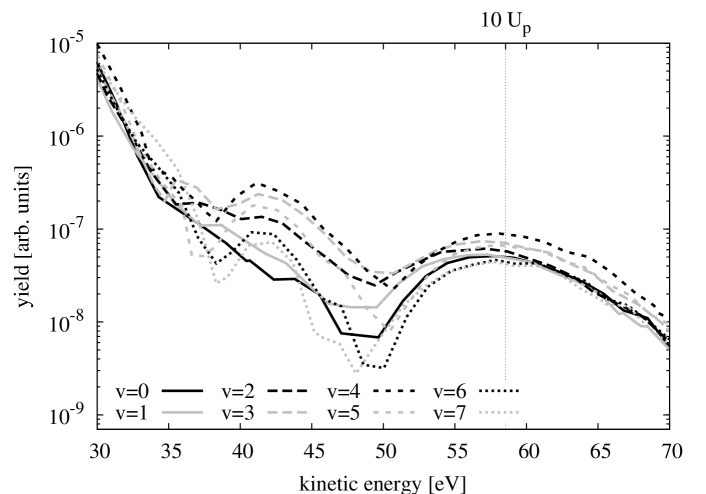
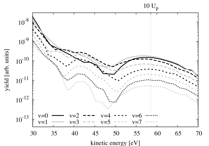
Figure 2: Envelopes of kinetic-energy spectra of (right-going) ATI electrons produced by a laser pulse of the intensity $I=9.696\times 10^{13}$ $\mathrm{W}/\mathrm{cm}^{2}$ ($U_{\mathrm{p}}=3.73~{}\omega$), plotted for vibrational states of the ${{\mathrm{H}_{2}}^{+}}$ ion from $v=0,\ldots,7$. In (a), the spectra are divided by the total yield of the corresponding vibrational state (cf. Fig. 3). In (b) the spectra show the correct weighting with respect to their yield.

In this case, in Eq. (2), $U_{\mathrm{p}}=3.73~{}\omega$ is kept fixed and $\Delta E^{v}$ is scanned from $v=0$ to $v=7$. This corresponds to values between $\Delta E^{0}=0.00~{}\omega$ and $\Delta E^{7}\approx 1.02~{}\omega$. The amount of energy the electron loses in each case as a consequence of energy conservation shifts the spectra with respect to each other. The ICC is masked by the fact that the different vibrational states are not populated equally (see Fig. 3).

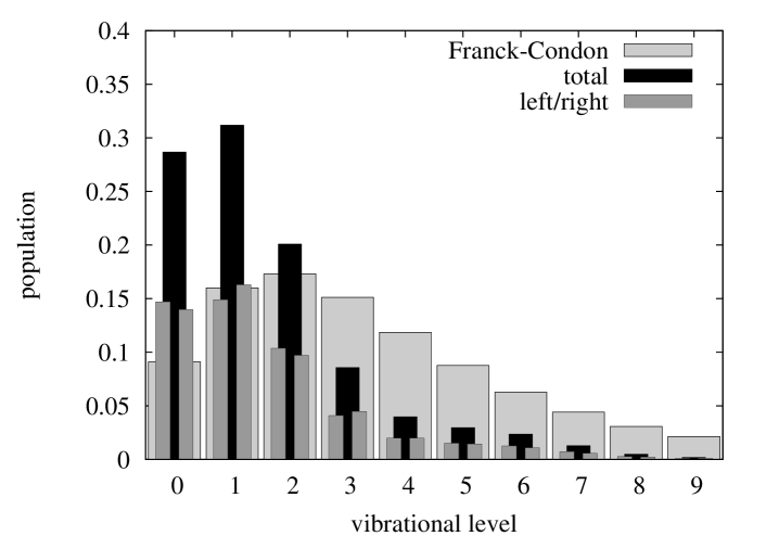
Figure 3: Occupation of vibrational states after a laser pulse with an intensity of $I=9.696\times 10^{13}\mathrm{W}/\mathrm{cm}^{2}$ ($U_{\mathrm{p}}=3.73~{}\omega$), split up into contributions from the left and right parts of the grid. The Franck-Condon overlap is plotted for comparison. The distribution has been normalized to total probability one .

Therefore, normalized spectra are plotted in Fig. 2(a), where each spectrum has been divided by the total yield of the corresponding vibrational state. The $v=4$ spectrum shows the highest yield in the middle hump compared to all other spectra within the plot. We attribute this behavior to an ICC. The unnormalized spectra in Fig. 2(b) show the highest yield of the middle hump already at $v=2$ due to the suppression of higher vibrational states. The application of Eq. (2) leads to $\Delta E^{v}=(k+0.31)~{}\omega$, where $k+14=n$, which corresponds to an energy difference close to the vibrational state $v=2$ (using $n=14$). Again, the observed position of the channel closing is shifted with respect to the one expected from Eq. (2).

It should be stressed that the energy difference between two vibrational states is larger than $0.1~{}\omega$ for all vibrational states considered in this work. Hence, in contrast to the intensity scanning, the transition over a channel closing is not sampled continuously. Similar calculations for $\mathrm{D}_{2}$ are work in progress and provide a finer graining due to the closer-lying vibrational states of the ${\mathrm{D}_{2}}^{+}$ ion.

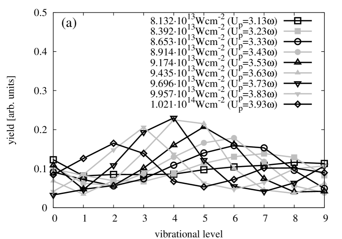
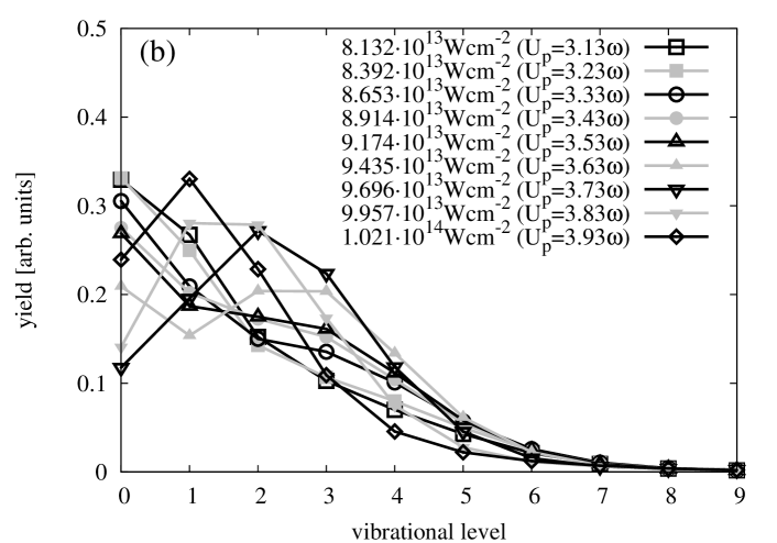
Figure 4: Electronic yield within the energy window $40$-$50$ eV (cf. Fig. 1), plotted versus vibrational states of the ${{\mathrm{H}_{2}}^{+}}$ ion for different laser intensities. In (a), the electron spectra used were divided by the total yield of the corresponding vibrational state (cf. Fig. 3) as in Fig. 2(a). In (b), correctly weighted spectra with respect to their yield were taken as in Fig. 2(b).

We show in Fig. 4, that for a suitable electron-energy window the ICC structure appears in the electron yield plotted as a function of vibrational quantum numbers. The distributions are shown using either the normalized electron yield from Fig. 2(a), see Fig. 4(a), or the unnormalized electron yield from Fig. 2(b), see Fig. 4(b). We use the energy window between 40 and 50 eV, corresponding to the dashed lines in Fig. 1. Clearly the ICC shows up in Fig. 4(a). Although the ICC feature is not as evident in the unnormalized distributions of Fig. 4(b), it is clearly visible that electrons and ions are highly correlated, since the distribution over vibrational states is, within the chosen electron-energy window, very different from the general distribution of vibrational states for all electrons. See, e.g., the curve for $U_{\mathrm{p}}=3.73~{}\omega$ as compared to Fig. 3.

To summarize, we found clear signatures of spectral enhancements due to channel closings occurring in ATI of ${\mathrm{H}_{2}}$ by scanning through the vibrational states of the created ${{\mathrm{H}_{2}}^{+}}$ ion. The explanation of this effect seems straightforward, applying energy conservation to the photon-absorbing molecule. Similar to atoms, we find that the effect occurs at intensities/vibrational states slightly different from the simple estimate based on the unperturbed ionization potential. We conclude with a note on the experimental perspectives. The populations of ${{\mathrm{H}_{2}}^{+}}$ vibrational states after strong-field ionization of ${\mathrm{H}_{2}}$ has been measured in Urbain et al. (2004), but a measurement in coincidence with electrons will be difficult. On the other hand, coincidence measurements similar to recent pump-probe experiments Ergler et al. (2006) appear feasible. The goal would be to measure the electron from an ionizing pump pulse, together with fragments from probe-pulse-induced Coulomb explosion of ${{\mathrm{H}_{2}}^{+}}$.

This work has been supported by the Deutsche Forschungsgemeinschaft.

References

- Agostini et al. (1979) P. Agostini, F. Fabre, G. Mainfray, G. Petite, and N. K. Rahman, Phys. Rev. Lett. 42, 1127 (1979).
- Eberly et al. (1991) J. H. Eberly, J. Javanainen, and K. Rza̧żewski, Phys. Rep. 204, 331 (1991).
- Paulus et al. (1994a) G. G. Paulus, W. Nicklich, H. Xu, P. Lambropoulos, and H. Walther, Phys. Rev. Lett. 72, 2851 (1994a).
- Paulus et al. (1994b) G. G. Paulus, W. Becker, W. Nicklich, and H. Walther, J. Phys. B 27, L703 (1994b).
- Paulus et al. (1995) G. G. Paulus, W. Becker, and H. Walther, Phys. Rev. A 52, 4043 (1995).
- Hansch et al. (1997) P. Hansch, M. A. Walker, and L. D. Van Woerkom, Phys. Rev. A 55, R2535 (1997).
- Hertlein et al. (1997) M. P. Hertlein, P. H. Bucksbaum, and H. G. Muller, J. Phys. B 30, L197 (1997).
- Muller and Kooiman (1998) H. G. Muller and F. C. Kooiman, Phys. Rev. Lett. 81, 1207 (1998).
- Muller (1999) H. G. Muller, Phys. Rev. A 60, 1341 (1999).
- Paulus et al. (2001) G. G. Paulus, F. Grasbon, H. Walther, R. Kopold, and W. Becker, Phys. Rev. A 64, 021401(R) (2001).
- Kopold et al. (2002) R. Kopold, W. Becker, M. Kleber, and G. G. Paulus, J. Phys. B 35, 217 (2002).
- Popruzhenko et al. (2002) S. V. Popruzhenko, P. A. Korneev, S. P. Goreslavski, and W. Becker, Phys. Rev. Lett. 89, 23001 (2002).
- Wassaf et al. (2003) J. Wassaf, V. Véniard, R. Taïeb, and A. Maquet, Phys. Rev. Lett. 90, 013003 (2003).
- Krajewska et al. (2006) K. Krajewska, I. I. Fabrikant, and A. F. Starace, Phys. Rev. A 74, 053407 (2006).
- Potvliege and Vučić (2006) R. M. Potvliege and S. Vučić, Phys. Rev. A 74, 023412 (2006).
- Kopold et al. (2000) R. Kopold, W. Becker, and M. Kleber, Opt. Commun. 179, 39 (2000).
- Bandrauk et al. (2003) A. D. Bandrauk, S. Chelkowski, and I. Kawata, Phys. Rev. A 67, 013407 (2003).
- Kreibich et al. (2001) T. Kreibich, M. Lein, V. Engel, and E. K. U. Gross, Phys. Rev. Lett. 87, 103901 (2001).
- Saugout et al. (2007) S. Saugout, C. Cornaggia, A. Suzor-Weiner, and E. Charron, Phys. Rev. Lett. 98, 253003 (2007).
- Urbain et al. (2004) X. Urbain, B. Fabre, E. M. Staicu-Casagrande, N. de Ruette, V. M. Andrianarijaona, J. Jureta, J. H. Posthumus, A. Saenz, E. Baldit, and C. Cornaggia, Phys. Rev. Lett. 92, 163004 (2004).
- Kołos et al. (1985) W. Kołos, K. Szalewicz, and H. J. Monkhorst, J. Chem. Phys. 84, 3278 (1985).
- Feuerstein and Thumm (2003) B. Feuerstein and U. Thumm, Phys. Rev. A 67, 043405 (2003).
- Chelkowski et al. (2007) S. Chelkowski, A. D. Bandrauk, A. Staudte, and P. B. Corkum, Phys. Rev. A 76, 013405 (2007).
- Grobe et al. (1999) R. Grobe, S. L. Haan, and J. H. Eberly, Comp. Phys. Comm. 117, 200 (1999).
- Löwdin (1955) P.-O. Löwdin, Phys. Rev. 97, 1474 (1955).
- Ergler et al. (2006) T. Ergler, A. Rudenko, B. Feuerstein, K. Zrost, C. D. Schröter, R. Moshammer, and J. Ullrich, Phys. Rev. Lett. 97, 193001 (2006).