The Rectilinar Three-body Problem using Symbol Sequence
II. Role of the periodic orbits

Abstract

We study the change of phase space structure of the rectilinear three-body problem when the mass combination is changed. Generally, periodic orbits bifurcate from the stable Schubart periodic orbit and move radially outward. Among these periodic orbits there are dominant periodic orbits having rotation number $(n-2)/n$ with $n\geq 3$. We find that the number of dominant periodic orbits is two when $n$ is odd and four when $n$ is even. Dominant periodic orbits have large stable regions in and out of the stability region of the Schubart orbit (Schubart region), and so they determine the size of the Schubart region and influence the structure of the Poincaré section out of the Schubart region. Indeed, with the movement of the dominant periodic orbits, part of complicated structure of the Poincaré section follow these orbits. We find stable periodic orbits which do not bifurcate from the Schubart orbit.

1 Introduction

In the present study, we continue our work on the rectilinear three-body problem (Saito & Tanikawa, 2007; hereafter referred to as Paper I). The rectilinear three-body system is such that three particles are on a line. This problem has two degrees of freedom.

The structure on the surface of section of the rectilinear three-body system has been studied using the Poincaré map ([Hietarinta & Mikkola, 1993]; hereafter HM1993). They found that the Poincaré section is divided into three basic regions: the Schubart region, the chaotic scattering region, and the immediate escape region. Inside the scattering region, the interplay time is so sensitive to the initial conditions that there seemed to be no structure. HM1993 also found that the number of scallops, which constitute the immediate escape region, increases as the mass of the central particle becomes smaller.

Tanikawa and Mikkola (2000a; hereafter referred to as TM2000a) studied the structure of the Poincaré section for the equal-mass case using symbol sequences which record the collisional history of orbits. They used the Poincaré section as the initial condition surface and associated with each point of the surface its future history including the final motion. They then succeeded in showing that the chaotic scattering region is filled with points whose orbits end with triple collision and that these points form well stratified curves. TM2000a’s fine structure of the Poincaré section for the equal-mass case shows that (1) stratified triple collision curves make a sector together with the sub-region of the immediate escape region (i.e., scallop); (2) four sectors surround the Schubart region.

The study of a similar dynamical system, the collinear Coulomb three-body problem with electron-ion-electron configuration, carried out by Sano (2003) is helpful to understand our system. In his system, there exist the Schubart region and unstable periodic points on its vertices. He confirmed the existence of the separatrices of these unstable points in his system numerically following the mapped points starting near the vertices.

In Paper I, we studied how the structure on the Poincaré section changes as the central mass varies. The chaotic scattering region is foliated with triple collision curves in general mass combination. This foliation makes two types of block: arch- and germ-shaped blocks (hereafter simply arches and germs; see Fig. 1). The chaotic scattering region consists only of arches near the mass combinations of total degeneracy, whereas it consists of arches and germs for the mass combinations away from total degeneracy. Here by total degeneracy we mean that stable and unstable manifolds of the two fixed points on the Triple Collision Manifold connect smoothly (McGehee, 1974). In the totally degenerate cases, the solutions can be analytically continued beyond triple collision. The number of arches always coincides with the number of the scallops. The mass combinations of total degeneracy are numerically found by Simó (1980). We introduced a family of sets of symbol sequences, and partitioned the Poincaré section by sets of points corresponding to sets of symbol sequences. We then found that an arch consists of sets of points whose symbol sequences are arranged according to a simple rule (see §4.1 of Paper I). The composition of arches changes each time the number of scallops increases, that is, the mass parameters pass through a totally degenerate case. We observed that a number of germs bifurcate from arches and then germs from different arches construct new arches. However, we could not understand the dynamics behind the behaviour of germs.

In the present paper, we also study the structure change of the Poincaré section as the central mass varies (we only consider the symmetric mass combinations). However, in contrast to Paper I, where the structure of the Poincaré section was considered in relation to triple collision, here the structure is analysed in relation to the motion of periodic orbits bifurcated from the Schubart orbit. From another point of view, the azimuthal structure of the Poincaré section with centre at the Schubart point has been studied in Paper I, whereas the radial structure with centre at the Schubart point will be studied in the present paper.

The rotation number with respect to the (Schubart) fixed point will be introduced. General tendency of the motion of the bifurcated orbits from the fixed point is analysed. The rotation number monotonically decreases as $a$ increases. As we shall see, there is the sequence of rotation numbers such that the corresponding periodic orbits has significant influence on the Poincaré section. these orbits will be called dominant periodic orbits. We mainly concern with these orbits. As the mass parameters change, the dominant periodic orbits bifurcate, recede from the fixed point, and their stability region shrink. We will relate these behaviours of periodic points to the growth of the germs observed in Paper I.

The organisation of the present paper is follows. In §2, we introduce the equations of motion of our system. We define the Poincaré section and introduce the rotation number in the fixed-point-centric coordinates. The §3 is for the results. In §3.1, the bifurcation of periodic points is analysed as the mass parameter changes. In §3.2, we find that periodic points with special rotation number are dominant over the structure of the Poincaré section. In §3.3, we show in detail the radial motion of the periodic point with the growth of the germs as the mass parameter changes. Finally in §4, we summarise our results.

2 Method

2.1 Equations of Motion and Initial Points

We introduce the equations of motion, the Poincaré section, and parameters describing mass combination of the particles (MH1989). Then, we introduce symbol sequences recording the collisional history of orbits (TM2000a).

Let $m_{1},m_{0}$, and $m_{2}$ denote the masses of the three particles from left to right on the line. Let $(q_{1},q_{2})$ be the mutual distances $\overline{m_{1}m_{0}}$ and $\overline{m_{0}m_{2}}$, and $(p_{1},p_{2})$ the conjugate momenta to $(q_{1},q_{2})$. The Hamiltonian $H$ is written, with the kinetic energy $K$ and the force function $U$, as

$$H = K-U,$$ (1)

$$K = \frac{1}{2}\Big{(}\frac{1}{m_{1}}\kern-1.99997pt+\kern-1.99997pt\frac{1}{m_{0}}\Big{)}p_{1}^{2}+\frac{1}{2}\Big{(}\frac{1}{m_{0}}\kern-1.99997pt+\kern-1.99997pt\frac{1}{m_{2}}\Big{)}p_{2}^{2}-\frac{p_{1}p_{2}}{m_{0}},$$

$$U = \frac{m_{1}m_{0}}{q_{1}}+\frac{m_{0}m_{2}}{q_{2}}+\frac{m_{1}m_{2}}{q_{1}+q_{2}}.$$

In this paper, we consider the case that total energy $E$, where $H=E=const.$, is negative. We restrict ourselves to $E=-1$, since negative energy system can be brought to $E=-1$ using the homogeneity of $U$. We here adopt variables used in MH1989. For readers’ convenience, we repeat the formulation. Let us consider the canonical transformation from $(q_{i},p_{i},t)$ to $(Q_{i},P_{i},t^{\prime})$ defined by

$$q_{i} = Q_{i}^{2},\ p_{i}=2p_{i}Q_{i}\ \ (i=1,2)$$ (2)

$$dt = q_{1}q_{2}dt^{\prime}.$$ (3)

Then the new Hamiltonian reads

$$\Gamma = q_{1}q_{2}(H-E),$$ (4)

and the equations of motion become

$$\frac{dQ_{i}}{dt^{\prime}}=\frac{\partial\Gamma}{\partial P_{i}},\quad\frac{dP_{i}}{dt^{\prime}}=-\frac{\partial\Gamma}{\partial Q_{i}}\quad(i=1,2).$$ (5)

The transformed equations (5) show that binary collisions ($Q_{1}=0,Q_{2}\neq 0$ or $Q_{2}=0,Q_{1}\neq 0$) are regularised, whereas triple collision ($Q_{1}=Q_{2}=0$) is still singular. The solution to Eq. (5) is continued beyond binary collision. A binary collision is interpreted as an elastic bounce in the physical coordinates.

The equations of motion allow a solution $q_{1}(t)=\Lambda q_{2}(t)$ for all $t$ for which the solution is defined. This is called the homothetic solution ([Irigoyen and Nahon, 1972]). Here $\Lambda$ is a constant depending on masses. This dependence is given by the following equation:

$$\frac{-m_{1}+zm_{0}+m_{2}}{m_{1}+m_{0}+m_{2}}=\frac{z^{5}-2z^{3}+17z}{z^{4}-10z^{2}-7}, {\rm where} \Lambda=\frac{1+z}{1-z}.$$ (6)

The intersection of the energy hyper-surface $H(q,p)=E$ and the hyper-surface $q_{1}=\Lambda q_{2}$ is a two-dimensional surface. We take this surface as the Poincaré section $\overline{\Pi}$. In the following, we introduce coordinates $(\theta,R)$ on $\overline{\Pi}$. The variable $R$ is defined by

$$R=\frac{1}{2}(q_{1}+q_{2})\quad{\rm where}\quad{q_{1}=\Lambda q_{2}}.$$ (7)

With solving Eq. (7) to obtain $q_{1}$ and $q_{2}$ for a given $R$, the value of $K$ is determined as

$$K=E+U(q_{1},q_{2})\quad{\rm with}\quad q_{1}=\frac{2\Lambda R}{1+\Lambda},\ q_{2}=\frac{2R}{1+\Lambda}.$$ (8)

For this value of $K$, the parameter $\theta$ determines the ratio of $\dot{q}_{1}$ to $\dot{q}_{2}$:

$$\kern-20.00003pt\sqrt{K}\cos\theta=\sqrt{A-\kappa{r_{2}}^{2}}\dot{q}_{1}-\sqrt{B-\kappa{r_{1}}^{2}}\dot{q}_{2}$$

$$\kern-20.00003pt\sqrt{K}\sin\theta=r_{2}\sqrt{\kappa}\dot{q}_{1}-r_{1}\sqrt{\kappa}\dot{q}_{2},$$ (9)

where

$$A=\frac{m_{1}(m_{0}+m_{2})}{2M},\ B=\frac{m_{2}(m_{0}+m_{1})}{2M},\ C=\frac{m_{2}m_{0}}{2M},\ M=m_{1}+m_{0}+m_{2},$$

$$r_{1}=\frac{2\Lambda}{\Lambda+1},\ r_{2}=\frac{2}{\Lambda+1},\ \kappa=\frac{4AB-C^{2}}{4(A{r_{1}}^{2}+B{r_{2}}^{2}+Cr_{1}r_{2})},\ 0\leq\theta<2\pi.$$

The variable $R$ takes its maximum value $R_{\rm max}$ when $K=0$. Substituting $K=0$ in Eq. (8), we obtain

$$R_{\rm max}=\frac{|E|}{2}\Big{[}\frac{\Lambda+1}{\Lambda}m_{0}m_{1}+(\Lambda+1)m_{0}m_{2}+m_{1}m_{2}\Big{]}.$$ (10)

We denote by $\Pi$ the side of the Poincaré section with $0\leq\theta<\pi$ and by $\Pi^{*}$ the other side with $\pi\leq\theta<2\pi$. By the definition of $\theta$ in Eq. (9), $\dot{\hbox{\bfit q}}(\theta+\pi)=-\dot{\hbox{\bfit q}}(\theta)$, where we denote by $\dot{\hbox{\bfit q}}(\theta)$ the $(\dot{q}_{1},\dot{q}_{2})$ for given $\theta$. Since the original equations of motion are invariant under the transformation $(\dot{q}_{i},t)\to(-\dot{q}_{i},-t)$, it is enough to integrate orbits toward the future for each point $(\theta,R)$ in $\Pi\cup\Pi^{*}$. Nonetheless, we only study the structure of the surface $\Pi$ for future integration. The reason why we do so is that an orbit intersects alternately with $\Pi$ and $\Pi^{*}$ until the corresponding triple system disintegrates into a binary and a single particle. Only certain orbits starting from the immediate escape region intersect with only $\Pi$ or $\Pi^{*}$. Since we are interested in the structure of chaotic scattering region, such escape orbits can be neglected.

We assume the total mass of the particles to be three without loss of generality and introduce parameters $a$ and $b$ to represent the masses:

$$\kern-30.00005ptm_{1}=1-a-b,\ m_{0}=1+2a,\ m_{2}=1-a+b,$$ (11)

$${\rm where}\ a>-1/2,\ b>0,\ a+b<1.$$

The parameters move in a triangular area of the $(a,b)$-plane. We will call this a mass triangle. In Paper I, we saw the structure change of the Poincaré section over the mass triangle. In the present paper, we only consider the symmetric mass configurations: $b=0$. The reason is that we saw in Paper I that asymmetry of the mass configuration in many cases does not add topologically new structure to the symmetric case.

There are three types of collision in our system: left-centre ($q_{1}=0,q_{2}\neq 0$), centre-right ($q_{2}=0,q_{1}\neq 0$), and triple ($q_{1}=q_{2}=0$) collisions. Let us denote these collisions by symbols ‘1’, ‘2’, and ‘0’, respectively. An orbit of the partly regularised equations Eq. (5) repeats binary collisions until a triple collision takes place. These collisions can be recorded as a sequence of the symbols. We study the evolution of orbits using the symbol sequences instead of orbits themselves. It is to be noted that we encode into symbol sequences the future behaviour of the orbits starting at points of the Poincaré section. So symbol sequences are not bi-infinite but singly infinite to the future.

Integration of orbits are carried out for grid points. We introduce the grid points $(\theta_{i},R_{i})$ with different resolution on $\Pi$:

$$(\theta_{i},R_{i})=(\pi\times\frac{i}{\theta_{\rm div}},R_{\rm max}\times\frac{j}{R_{\rm div}}),\hbox{ where }i=0,\cdots,\theta_{\rm div}-1,\ j=1,\cdots,R_{\rm div},$$

$$\hskip 40.00006pt\raise 6.45831pt\hbox{and }\left\{\begin{array}[]{ll}{\rm(i)}&\theta_{\rm div}=540,\ R_{\rm div}=300\\ {\rm(ii)}&\theta_{\rm div}=1800,\ R_{\rm div}=1000\end{array}\right.$$ (14)

Most of structures on the Poincaré section and their change due to the mass variation can be resolved with resolution (i). Detailed structures may be lost, if one uses resolution (i). However, once we understand certain fine structures with resolution (ii), we can use resolution (i) to follow global behaviour of the structure of the Poincaré section when mass parameters are changed. We have obtained the first 64 digits of symbol sequences for the grid points through integration of orbits. These constitute the basic data in the rest of the paper for the distribution of symbol sequences on $\Pi$. We integrate Eq. (5) using DIFSY1, which is an implementation ([Press and Teukolsky, 1999]) of Bulirsch-Stoer method. In our preliminary research ([Saito & Tanikawa, 2004]), we introduced cylinders (sets of symbol sequences with given words where a word is a finite sequence of symbols) $S_{c,j}$, $S_{c,\infty}$ and $S_{c}$:

$$S_{c,j}\equiv\left\{\begin{array}[]{l}{\{(21)^{i}(2)^{j}\cdots|i\geq 0,j\geq 1\}}\quad{\rm for}\ {c=2i+1}\\ {\{(21)^{i}(1)^{j}\cdots|i\geq 1,j\geq 1\}}\quad{\rm for}\ {c=2i}\end{array}\right.$$ (17)

$$S_{c,\infty}\equiv\left\{\begin{array}[]{l}{\{(21)^{i}(2)^{\infty}|i\geq 0}\}\quad{\rm for}\ {c=2i+1}\\ {\{(21)^{i}(1)^{\infty}|i\geq 1}\}\quad{\rm for}\ {c=2i}\end{array}\right.$$ (20)

$$S_{c}\equiv\cup_{j<\infty}S_{c,j}.$$ (21)

Let ${\rm reg}(c)$ and ${\rm reg}((c,\infty))$ denote the regions on $\Pi$ whose symbol sequences belong to $S_{c}$ and $S_{c,\infty}$. The three basic regions in HM1993 correspond to our regions as follows:

Immediate escape region	${\rm reg}((c,\infty))$	$1\leq c\leq n_{\rm FOP}$
Chaotic scattering region	${\rm reg}(c)\cup{\rm reg}((c^{\prime},\infty))$	$1\leq c<\infty,\ n_{\rm FOP}+1\leq c^{\prime}<\infty$
Schubart region	${\rm reg}(c)$	$c=\infty$

.

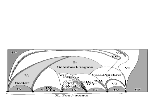
Figure 1: The schematic illustration of the structure on the Poincaré section. The Poincaré section consists of the Schubart region (I) and sectors (V). A sector (V) includes one scallop (IV), one arch (VI), and optional germs (VII) and pipelines (VIII). In the third sector from the left, it is shown that both an arch and a germ consist of the strata of triple collision curves. In the blank area of the third sector, there are other germs and/or pipelines, although they are not drawn. The pipeline (VIII) is an object which connects two germs in different sectors. Note that there are narrow escape regions also inside the sectors.

For later convenience, we recall the structure of the Poincaré section and names for its elements obtained in Paper I (Fig. 1). The separatrices running from the vertices of (I) the Schubart region divide the outside of the Schubart region into (V) sectors. A sector includes (IV) one scallop. In the remainder of the sector, (IX) triple collision curves are foliated. This foliation makes one or more blocks. One block is arch-shaped (VI, arch) and the other blocks are germ-shaped (VII, germ). A germ bifurcates from an arch, as $a$ changes. Germs that bifurcate from different arches finally gather to construct a new arch and to reconstruct other arches. As is shown later, the growing process of germs is related to the movement of the periodic orbits bifurcated from the Schubart orbit.

2.2 Poincaré map and rotation number

We here define the Poincaré map on the Poincaré section $(\theta,R)$. An orbit starting from the Poincaré section repeats the intersection with $\Pi$ and $\Pi^{*}$ alternately. When an orbit intersects with $\Pi$ (resp. $\Pi^{*}$) at $(\theta,R)$ and $\Pi$ (resp. $\Pi^{*}$) again at $(\theta^{\prime\prime},R^{\prime\prime})$, we define a map T from $(\theta,R)$ to $(\theta^{\prime\prime},R^{\prime\prime})$.

$$T:(\theta,R)\mapsto(\theta^{\prime\prime},R^{\prime\prime}),\hbox{ where }(\theta,R),(\theta^{\prime\prime},R^{\prime\prime})\in\Pi\hbox{ or }(\theta,R),(\theta^{\prime\prime},R^{\prime\prime})\in\Pi^{*}$$ (22)

Equation (5) has a simple periodic solution, the so-called Schubart orbit (Schubart, 1956), whose symbol sequence is $(21)^{\infty}$. The intersection $\hbox{\bfit P}_{0}=(\theta_{0},R_{0})$ of the Schubart orbit with $\Pi$ is a fixed point of the map, namely $\hbox{\bfit P}_{0}=T(\hbox{\bfit P}_{0})$. The linear stability of $T$ around $\hbox{\bfit P}_{0}$ over the mass triangle is studied by HM1993. Approximately in the mass combinations such that $m_{1}<m_{0}<m_{2}$, $\hbox{\bfit P}_{0}$ is hyperbolic whereas in the other combinations it is elliptic. The stability region is called the Schubart region. A point P such that $\hbox{\bfit P}=T^{q}(\hbox{\bfit P})$ is called a q-periodic point and the sequence $\{\hbox{\bfit P},T^{1}(\hbox{\bfit P}),\cdots,T^{q-1}(\hbox{\bfit P})\}$ is called a q-periodic orbit. We are interested in the periodic orbits that bifurcate from the fixed point as the mass parameter $a$ is changed.

In order to describe the elliptic motion around $\hbox{\bfit P}_{0}$, we introduce the rotation number. The rotation number is the averaged number of rotations per iterate of $T$. First, we introduce polar coordinates $(D,A)$ with centre at $\hbox{\bfit P}_{0}=(\theta_{0},R_{0})$:

$$D\cos A=(\theta-\theta_{0}){\rm g}_{\theta},\quad D\sin A=(R-R_{0}){\rm g}_{R},$$

where $\quad{\rm g}_{\theta}=180/\pi$ and $\quad{\rm g}_{R}=100/R_{\rm max}$. The values of ${\rm g}_{\theta}$ and ${\rm g}_{R}$ are arbitrarily chosen such that both $\theta$ and $R$ equally contribute to the values of $D$ and $A$. Now the Poincaré map is expressed as $T:(D,A)\mapsto(D^{\prime},A^{\prime})$. We then introduce the effective rotation number $\nu_{n}(D,A;a)$ and the (exact) rotation number $\nu_{\infty}(D,A;a)$ at $(D,A;a)$ in the following equations:

$${\rm diff}(A^{\prime},A)=\bigg{\{}\begin{array}[]{ll}A^{\prime}-A&({\rm if}\ A^{\prime}-A\geq 0)\\ A^{\prime}-A+2\pi&({\rm if}\ A^{\prime}-A<0)\end{array}$$ (25)

$$\nu_{n}((D,A);a)=\frac{1}{2n\pi}\sum_{i=1}^{n}{\rm diff}(A^{(i)},A^{(i-1)}),\quad{\rm where}\ (D^{(i)},A^{(i)})=T^{i}(D,A)$$ (26)

$$\nu_{\infty}((D,A);a)=\lim_{k\to\infty}\nu_{k}(D,A;a)\kern 20.00003pt\hbox{(if the limit exists)}.$$ (27)

We here remark several points related to the numerical calculation of the rotation number. The first point is the selection of $n$ of the $\nu_{n}((D,A);a)$. In our approach, we first take an fixed integer $N$ and iterate the mapping $N$ times. We then find a number $n$ ($1\leq n\leq N$) such that ${\rm diff}(A^{(n)},A)=\min_{1\leq i\leq N}\{{\rm diff}(A^{(i)},A)\}$. The second point concerns the rotation number of periodic points. Suppose $p$ and $q$ are integers. If P is a periodic point, then there exist integers $p$ and $q$ such that $\nu_{q}(\hbox{\bfit P};a)=\nu_{\infty}(\hbox{\bfit P};a)=p/q$ (by the above method of selection of $n$, $n=q$). This coincidence of the effective and exact rotation numbers helps us to find the periodic points: the points on the contour with $\nu_{q}(\hbox{\bfit P};a)=p/q$ on the the Poincaré section are the candidates of the periodic points with $\nu_{\infty}(\hbox{\bfit P};a)$. The third point is that the rotation number $\nu_{\infty}(\hbox{\bfit P}_{0};a)$ is calculated from the eigenvalues of linearised map of $T$ at $P_{0}$. When this value is rational, the fixed point and the periodic points are degenerated. If the mass parameter $a$ is changed, the periodic points bifurcate from fixed point $\hbox{\bfit P}_{0}$.

2.3 Search for the periodic points

We explain how to detect the periodic points. First, we have to calculate $\lim_{D\to 0}\nu_{\infty}((D,A);a)$ for various values of $a$. For a given rotation number $p/q$, we can determine the mass parameter $a$ where corresponding periodic points appear: solve $\nu_{\infty}(\hbox{\bfit P}_{0};a)=p/q$ for $a$. Second, we find candidates at a mass parameter a little distant from the exact bifurcation. The candidates for periodic points are found from the Poincaré map such as is shown in Fig. 2. The candidates for elliptic points can be taken at the centre of the libration and for hyperbolic points at the saddle between two librations.

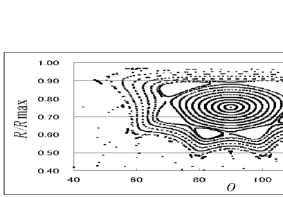
Figure 2: A Poincaré map in order to select candidates for periodic points. In this map, $a=-0.25$ and the expected periodic points are those with $\nu=4/6$. The centres of elliptic motions under the Poincaré map are the candidates.

Finally, we obtain a periodic point through the Newton-Raphson method Eq. (28) starting from an arbitrary point on the contour. This method is used in MH1991 to find the fixed point.

$$\vec{X}_{n+1}=\vec{X}_{n}-\Bigg{[}\frac{\partial T(\vec{X}_{n})}{\partial\vec{X}_{n}}-1\Bigg{]}^{-1}(T^{p}(\vec{X}_{n})-\vec{X}_{n})=0.$$ (28)

3 Results

We now show the behaviour and influence of the periodic points on the Poincaré section. First, their bifurcation and radial movement away from the Schubart orbit will be discussed. The values of parameter $a$ where the periodic points bifurcate can be determined from the rotation number, $\nu_{\infty}({\hbox{\bfit P}_{0}};a)$, of the Schubart orbit as a function of $a$. The relation between radial movement and the variation of $a$ will be studied. Second, the number of orbits which appear in respective bifurcations for special rotation numbers will be discussed. Finally, the influence of such special periodic orbits on the Poincaré section will be discussed.

3.1 Bifurcation as the parameter changes

In this subsection, we show how periodic points bifurcate and move outward from the fixed point $\hbox{\bfit P}_{0}$, when the parameter $a$ is changed. As is stated in section 2.2, period-$q$ points bifurcate if $\nu_{\infty}(\hbox{\bfit P}_{0};a)=p/q$ with integers $p$ and $q$. In order to know when the periodic orbits bifurcate, we calculate $\nu_{\infty}(\hbox{\bfit P}_{0};a)$ as a function of $a$ (Fig. 3). For several rotation numbers, we show the values of $a$ in Table 1. Figure 3 shows $\nu_{\infty}(\hbox{\bfit P}_{0};a)$ is monotonic:

$$\frac{\partial\nu_{\infty}(\hbox{\bfit P}_{0};a)}{\partial a}<0.$$ (29)

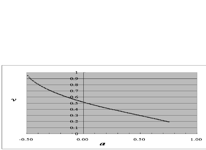
Figure 3: The rotation number $\nu(\hbox{\bfit P}_{0},a)$ as a function of $a$.

Therefore for each rational number $p/q$, the periodic points with $\nu_{\infty}=p/q$ bifurcate once and for all.

$\nu_{\infty}$	1/4	1/3	2/4	3/5	4/6	3/7
$a$	0.61	0.41	-0.019	-0.15	-0.25	-0.31

Table 1: The values of $a$ at which the periodic points bifurcate for several rotation numbers

Note that this graph shows that the period-3 orbit bifurcates at $a=a_{1/3}\hbox{\kern 2.29996pt\raisebox{4.79996pt}{.}\kern-2.29996pt=\kern-2.79999pt\raisebox{-1.00006pt}{.}\kern 2.79999pt}0.41$. According to Moser (1958), generally in Hamiltonian systems when the period-3 orbit bifurcates, the mother periodic orbit becomes unstable. As an application of this result, he tried to explain the origin of the Kirkwood gaps. Also in our system, the instability at the bifurcation of the period-3 orbit was confirmed by Hietarinta and Mikkola (1993). We have followed the position of the periodic points with $\nu_{\infty}=1/3$ on the Poincaré section with continuously changing $a$. As a result, when $a$ is decreased, with a passage $a=a_{1/3}$, the triangle formed by these periodic points approaches ($a>a_{1/3}$), collides ($a=a_{1/3}$) with, and recedes ($a<a_{1/3})$ from $\hbox{\bfit P}_{0}$ (Fig. 4(a)). The orientation of the triangle is inverted before and after $a_{1/3}$ (Fig. 4(b)). Similar behaviour was observed by Hénon (1970) in Hill’s case of the restricted three-body problem. In his case, mother periodic orbit is the retrograde satellite orbit.

(a) The distance from $\hbox{\bfit P}_{0}$

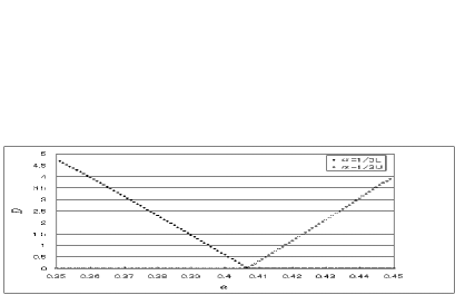
(b) The inversion of triangle’s orientation

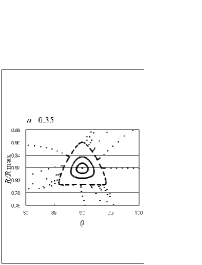
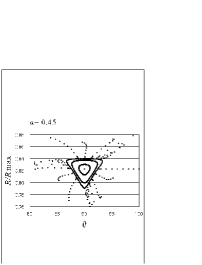
Figure 4: The radial movement of the periodic points with $\nu_{\infty}=1/3$ from $\hbox{\bfit P}_{0}$. (a) the distance between one of these point and $\hbox{\bfit P}_{0}$.

We want to know the direction of change of $a$ for the bifurcated periodic points to move outward from $\hbox{\bfit P}_{0}$. Suppose that the periodic points bifurcate at $a=a_{p/q}$ and exist at $a=a_{p/q}+da$ as the points with a finite distance $dD$ from $\hbox{\bfit P}_{0}$. The sign of $da$ can be obtained from Eqs.(29) and (31), as follows. The total differential of $\nu$ as a function of $a$ and $D$ at $\hbox{\bfit P}_{0}$ is

$$d\nu=\Big{(}\frac{\partial\nu}{\partial a}\Big{)}\Big{|}_{\hbox{\bfit P}_{0}}da+\Big{(}\frac{\partial\nu}{\partial D}\Big{)}\Big{|}_{\hbox{\bfit P}_{0}}dD.$$

Since $d\nu=0$ on periodic points, we obtain

$$da=-\Big{(}\frac{\partial\nu}{\partial D}\Big{/}\frac{\partial\nu}{\partial a}\Big{)}\Big{|}_{\hbox{\bfit P}_{0}}dD.$$ (30)

We only need the sign of $\partial\nu_{\infty}(\hbox{\bfit P}_{0};a)/\partial D$, since we already know the sign of $\partial\nu_{\infty}(\hbox{\bfit P}_{0};a)/\partial a$. We approximate the derivative $\partial\nu_{n}(\hbox{\bfit P};a)/\partial D$ by the difference $(\nu_{n}((D+\Delta D,A);a)-\nu_{n}((D,A);a))/\Delta D$ for small $\Delta D$. Since $\partial\nu_{n}(\hbox{\bfit P}_{0};a)/\partial D$ should be independent to $A$, we select arbitrarily the value of $A$: $A=0$. Moreover, we have $\nu_{\infty}(\hbox{\bfit P}_{0};a)\hbox{\kern 2.29996pt\raisebox{4.79996pt}{.}\kern-2.29996pt=\kern-2.79999pt\raisebox{-1.00006pt}{.}\kern 2.79999pt}\nu_{n}(\hbox{\bfit P}_{0};a)$ for large $n\leq N$: $N=256$. Finally we put $\Delta D=0.1$. Figure 5 shows $\partial\nu_{\infty}(\hbox{\bfit P}_{0};a)/\partial D$ as a function of mass parameter $a$. The figure shows that the sign of $\partial\nu_{\infty}(\hbox{\bfit P}_{0};a)/\partial D$ is

$$\left\{\begin{array}[]{cc}\displaystyle\frac{\partial\nu_{\infty}(\hbox{\bfit P}_{0};a)}{\partial D}>0&(\hbox{for }a>a_{1/3})\\ \raise 17.22217pt\hbox{}\displaystyle\frac{\partial\nu_{\infty}(\hbox{\bfit P}_{0};a)}{\partial D}<0&(\hbox{for }a<a_{1/3})\\ \end{array}\right.$$ (31)

Taking into account Eqs.(29) and (31), and $dD>0$, we find that $da$ is positive for $a>a_{1/3}$ and negative for $a<a_{1/3}$. The recession from $a=a_{1/3}$, irrespective of the sign of $a$, yields successive recessions of the periodic points from the Schubart orbit. This implies that absense of the periodic points at $a=a_{1/3}$ (except for the periodic points independent of $\hbox{\bfit P}_{0}$).

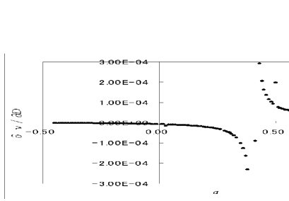
Figure 5: Dependence of $\partial\nu(D,a)/\partial D$ on $a$. The sign of $\partial\nu(D,a)/\partial D$ changes at $a=a_{1/3}$.

3.2 Dominant Periodic Orbits

In the present subsection, we will find periodic orbits and follow their motions for various rotation number. These results show us that the periodic orbits with rotation number $(n-2)/n$ dominate the structure of the Poincaré section. We call these the dominant periodic orbits. We discuss a few features of the dominant periodic orbits. On the other hand, periodic orbits with the other rotation numbers have too small stable regions to numerically find the location on the Poincaré section, so we do not consider these.

According to our numerical results, there is a rule for the number of dominant periodic orbits. Suppose that the rotation number of these orbits is $\nu_{\infty}=(n-2)/n$. Indeed, for even $n$, the period is not $n$ but $n/2$, and therefore, if we would strictly write the rotation number, it should be $\nu_{\infty}=(n/2-1)/(n/2)$. We have found the following rule for the number of periodic points.

A Rule

For the number of dominant periodic orbits with $\nu_{\infty}=(n-2)/n$, the following rule is confirmed from $n=4$ to $n=19$.

• the number of orbits is two for odd $n$.

• the number of orbits is four for even $n$.

We show an example of this rule in Fig. 6 ($n=5$ and 6) and Fig. 7 ($n=17$ and 18). For the case of $n=3$ ($\nu_{\infty}=1/3$), only one unstable orbit appears through bifurcation as already seen in Fig. 4(b). It is important to note that according to the Poincaré-Birkhoff theorem ([Birkhoff, 1913]) the number of the periodic orbits is $2\ell$ with an integer $\ell$, and in the case of the standard map ([Chirikov, 1979]) $\ell$ is believed to be one. We do not know the number of non-dominant orbits.

(a) $\nu=3/5$

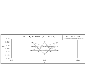
(b) $\nu=4/6$

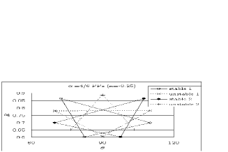
Figure 6: Periodic orbits for $\nu_{\infty}=(n-2)/n$ with (a) $n=5$ and (b) $n=6$. These show the numbers of orbits are 2 for odd $n$ and 4 for even $n$. We connect the periodic points which belong to the same orbit.

(c) $\nu=15/17$, $(a,b)=(-0.461844,0)$

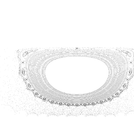
(d) $\nu=16/18$, $(a,b)=(-0.466010,0)$

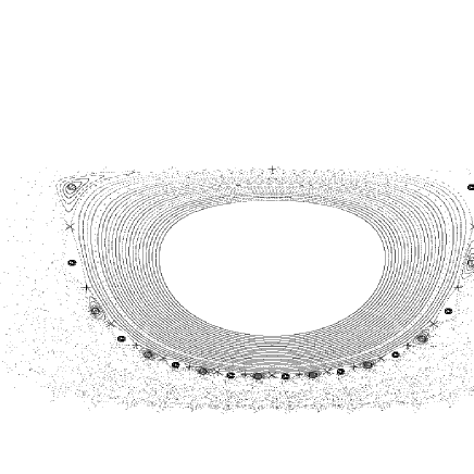
Figure 7: Periodic orbits for $\nu_{\infty}=(n-2)/n$ with (a) $n=17$ and $n=18$. For each orbit, its orbital points are plotted by different symbols: single and double circles (stable orbits), multiplicative and additive symbols (unstable orbits). Two symbols appear for odd case ($n=17$), whereas four symbols do for even case ($n=18$). The background dots shows the Poincaré map of segments of several lines running from $\hbox{\bfit P}_{0}$.

3.3 Periodic orbits and the structure on the Poincaré section

In the present subsection, we study how the dominant periodic orbits are related to the structures on the Poincaré section.

Because of the reversal of the bifurcation at $a=a_{1/3}$, we observe different movements of periodic orbits for two cases: $da>0$ for $a>a_{1/3}$, and $da<0$ for $a<a_{1/3}$. In the latter case, there is a nearly periodic change of the Poincaré section, and one cycle is from the bifurcation with $\nu_{\infty}=(n-2)/n$ to that with $\nu_{\infty}=\{(n+1)-2\}/(n+1)$. The change in the former case is basically similar to the one cycle in the latter case (Note that for $a>a_{1/3}$ only $\nu_{\infty}=1/3$ has the form $\nu_{\infty}=(n-2)/n$). Hence, we propose the scenario for the latter case only. The following scenario is based on the observation of the cycles starting respectively at $\nu_{\infty}=2/4,3/5$, 4/6, 5/7, and 6/8.

We explain our scenario referring to Fig. 8 which corresponds to the cycle starting at $\nu_{\infty}=3/5$. The bifurcated periodic points with $\nu_{\infty}=(n-2)/n$ ($n\geq 4$) recede from $\hbox{\bfit P}_{0}$ as $a$ decreases. As the distances become large, the stable regions around the periodic points, called islands, influence the shape of the Schubart region. In both Fig. 8 (a) and (b), five triangular islands can be seen. The separatrices which connect the unstable periodic points (and envelope the stability region of the stable ones) is of polygramic shape. The germs (see Section 2.1) grow along the separatrix. That makes the Schubart region be of polygramic shape. When the periodic points together with their islands get out of the Schubart region, the Schubart region returns to the polygonal shape. The germs now intrude between the Schubart region and islands. As $a$ further decreases, the stable periodic points sink into the gaps between arches, and their islands shrink. The germs grow and follow the sinking stable periodic points. As a result, a set of germs pile up over an arch. The piled germs become a new arch. On the contrary, the unstable periodic points stay around the vertices of the Schubart region: their separatrix approximates the boundary of the Schubart region. If we continue to decrease $a$, the next dominant periodic orbits with $\nu_{\infty}=\{(n+1)-2\}/(n+1)$ bifurcate. The evolution of the structure of the Poincaré section following this bifurcation is similar to the case $\nu=(n-2)/n$. It is to be note that there seems to be a correspondence between the structure around the Schubart orbit (the fixed point) and a structure around a bifurcated periodic point. Around the Schubart orbit, there are the Schubart region and a number of arches, while around a bifurcated periodic point there are the islands and the region filled with germs.

In what follows, let us see numerical evidence that supports our scenario. For this purpose, we follow the change of the Poincaré section over the range of $a$ corresponding to $\nu_{\infty}=3/5$ and 4/6. In Fig. 8, the periodic points on the Poincaré section for the range $-0.150\geq a\geq-0.250$ are displayed. The structure of the Poincaré section is represented in two ways: the triple collision curve and the partitioning according to the cylinders defined by Eq. (21). The separatrices of the periodic points are also plotted.

The radial recession of the periodic points and the enlargement of the islands, as $a$ decreases, can be seen in Fig. 8 (a) $a=-0.150$ and (b) $a=-0.160$. The germs grow along the separatrix which encloses the islands at (b) $a=-0.160$, whereas the germs split the Schubart region and the islands at (c) $a=-0.166$. This means that the periodic points get out of the Schubart region at $a^{\prime}$ such that $-0.166\leq a^{\prime}\leq-0.160$. After getting out of the Schubart region, islands become smaller. This is seen from the transition from (c) $a=-0.166$ to (d) $a=-0.170$.

The comparison of (d) $a=-0.170$ and (e) $a=-0.186$ shows us that the germs grow and follow the stable periodic orbit which is sinking between arches, and this growth of the germs results in the reconstruction of arches. For example, the second arch from the left has reg(2), reg(6), and other small regions at (b) $a=-0.160$, whereas reg(2), reg(7), reg(12), and other regions at (e) $a=-0.186$. Note that the head of the germ ${\rm reg}(5,\cdots)$ (the upper right in (e)) does not reach the $\theta$-axis and the number of arches is still four. The reconstruction process was studied well in Paper I. However, we have now found that this is promoted by the periodic orbits. Again in (e) $a=-0.186$, the unstable periodic points marked as five open circles stay at the vertices of the Schubart region. On the other hand, the stable periodic points marked as remaining five open circles are on the midway to the foot-points, although the stable region is no longer visible. The non-dominant orbits with $\nu_{\infty}=7/11$ have moderate distance from the Schubart orbit at (f) $a=-0.210$ and arrive at the boundary of the Schubart region at (g) $a=-0.230$. Since the stable regions are small, they are less effective to the shape of the Schubart region than the dominant periodic orbits. The number of arches is five already in (f) $a=-0.210$. According to Paper I, the number of arches becomes five at the totally degenerate case ($a\hbox{\kern 2.29996pt\raisebox{4.79996pt}{.}\kern-2.29996pt=\kern-2.79999pt\raisebox{-1.00006pt}{.}\kern 2.79999pt}-0.208)$ when the germs ${\rm reg}(5,\cdots)$ touch the $\theta$-axis. It is important to note that the value of $a$ such that the dominant periodic orbits bifurcate is far from that of total degeneracy. The next dominant orbits with $\nu_{\infty}=4/6$ exist at (h) $a=-0.250$. In this case, since there is two stable orbits, while their period is three, the number of islands is six. This makes, as a result, the separatrix be of hexagram shape. The periodic points with $\nu_{\infty}=3/5$ still exist at the place marked with $u_{i}$.

(a) $(a,b)=(-0.150,0)$

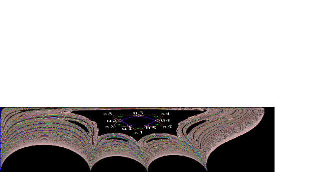
(b) $(a,b)=(-0.160,0)$

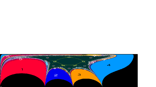
(c) $(a,b)=(-0.166,0)$

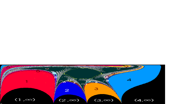
Figure 8: The periodic points and the separatrix on the Poincaré section for $\nu=3/5$

(d) $(a,b)=(-0.170,0)$

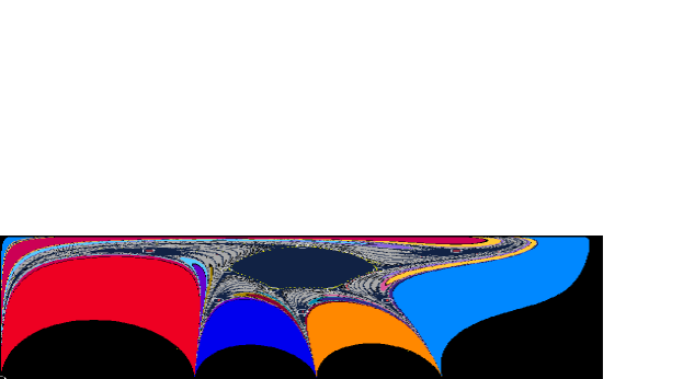
(e) $(a,b)=(-0.186,0)$

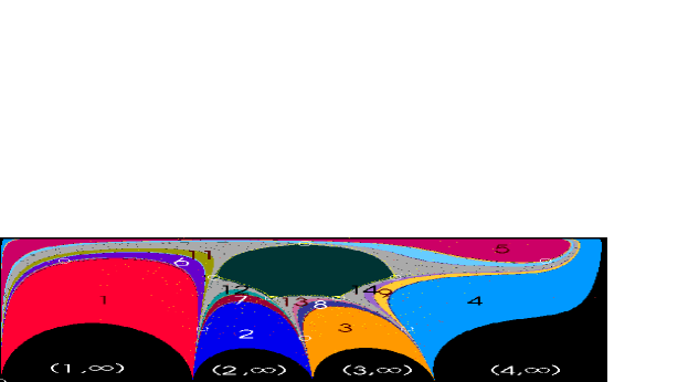
(f) $(a,b)=(-0.210,0)$

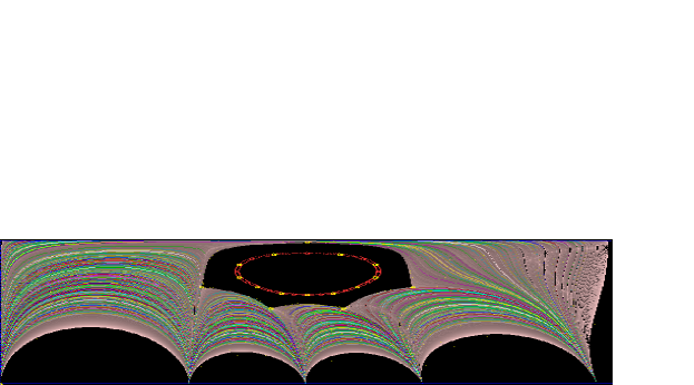
Figure 8: (continue)

(g) $(a,b)=(-0.230,0)$

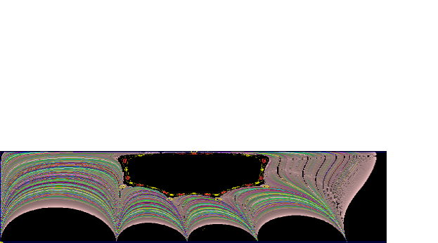
(h) $(a,b)=(-0.2500,0)$

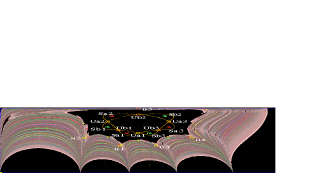
Figure 8: (continue)

4 Summary

We have studied the movement of the periodic points bifurcated from the fixed point (the Schubart orbit) and their influence on the structure of the Poincaré section for symmetric mass configuration. The following is the summary of the present paper.

• The periodic orbits with $\nu=(n-2)/n$, $n$ being integer, are influential on the structure of the Poincaré section. There is a rule about the number of orbits for these type orbits. A pair of stable and unstable orbits with period $n$ bifurcate for odd $n$, while two pairs bifurcate for even $n$.

• There is a value $a=a_{1/3}$ where the rotation number $\nu$ at the fixed point is 1/3. Whether $a$ is less or greater than $a_{1/3}$, as $|a-a_{1/3}|$ increases, the periodic orbits bifurcate from the Schubart orbit one after another. As a result, there are no periodic orbits bifurcated from the Schubart orbit at $a=a_{1/3}$.

• While the periodic points are inside the Schubart region, the germs, which bifurcate from arches grow along the separatrix of polygramic shape. The Schubart region takes also polygram shape. After the periodic points go out of the Schubart region, the Schubart region becomes polygonal. The germs grow along this polygon.

• The stable periodic points leave the fixed point quickly. They collect germs and sink toward the $\theta$-axis. This collection of germs results in re-composition of arches. On the other hand, the unstable periodic points stay at the vertices of the Schubart region for long time.

• At the moment of the bifurcation of the dominant periodic orbit for $\nu_{\infty}=(n-2)/n$, the number of arches is still $n-1$.

Several problems are remained unsolved. First, we could not determine where the stable periodic points tend to. One possible answer is to reach the foot-points. Second, the place where the unstable periodic points should finally go is also unclear. Third, we have found that two stable orbits bifurcate, when $(n-2)/n$ is divisible by 2. The possibility that three or more (non-dominant) periodic orbits bifurcate is unknown. Fourth, we have not considered the periodic orbits which do not bifurcate from the Schubart orbit. For example, in Fig. 8 (a) $a=-0.15$, there are four black regions inside arches (one region for one arch). We have confirmed that there are two period-2 orbits inside these regions such that one has its orbital point in the first and the third arches and the other in the second and the fourth arches. These periodic orbits has a different symbol sequence, $(21121)^{\infty}$, from that of the Schubart orbit.

References

- Mikkola & Hietarinta, 1989 S.Mikkola and J.Hietarinta, A numerical investigation of the one-dimensional Newtonian three-body problem I, Celestial Mechanics and Dynamical Astronomy 46, 1-18(1989)
- Mikkola & Hietarinta, 1991 Mikkola, S., Hietarinta, J.: A numerical investigation of the one-dimensional Newtonian three-body problem III. Celestial Mechanics and Dynamical Astronomy 51, 379-394 (1991)
- Hietarinta & Mikkola, 1993 Hietarinta, J., Mikkola, S.: Chaos in the one-dimensional gravitational three-body problem. CHAOS 3, 183-203 (1993)
- Tanikawa & Mikkola, 2000a Tanikawa, K., Mikkola, J.: Triple collisions in the one-dimensional three-body problem. Celestial Mechanics and Dynamical Astronomy 76, 23-34(2000)
- Tanikawa & Mikkola, 2000b Tanikawa, K., Mikkola, J.: One-dimensional three-body problem via symbolic dynamics, CHAOS 10, 649-657(2000)
- Saito & Tanikawa, 2004 Saito, M.M., Tanikawa, K.: Collinear Three-Body Problem with Non-Equal Masses by Symbolic Dynamics. ASP Conference Series 316, 63-69(2004)
- Simó 1980 Simó, C., Mass for which triple collision regularizable. Celestial Mechanics 21, 25-36(1980)
- Irigoyen and Nahon, 1972 Irigoyen, M. Nahon, F.: Les mouvements rectilignes dans le probléme des trois corps lorsque la constante des forces vives est nulle. Astronomy & Astrophysics 17, 286-295(1972)
- McGehee, 1974 McGehee, R.: Triple collision in the collinear three body problem. Inventiones Mathematicae 27, 191-227(1974)
- Moser, J.: Stability of the asteroids, Astronomical Journal 63, 439-443(1958)
- Hénon, M.: Numerical Exploration of the Restricted Problem. VI. Hill’s Case: Non-Periodic Orbits. Astron. & Astrophys. 9, 24-36(1970)
- Chirikov, 1979 Chirikov, B.V., A universal instability of many-dimensional oscillator systems. Phys. Rep. 52, 263-379(1979).
- Birkhoff, 1913 Birkhoff, G.D., Proof of Poincaré’s geometric theorem. Trans. Amer. Math. Soc. 14, 14-22(1913).
- Schubart, 1956 Schubart, J.: Losungen im Dreikörperproblem. Astronomische Nachrichten 283, 17-22(1956)
- Press and Teukolsky, 1999 Press W.H., Teukolsky S.A., Vetterling W.T., Flannery B.P.: Numerical Recipes in C, 722-724 (1999)