Absolute kinematics of radio source components
in the complete S5 polar cap sample

We report on the first wide-field, high-precision astrometric analysis of the 13 extragalactic radio sources of the complete S5 polar cap sample at 15.4 GHz. We describe new algorithms developed to enable the use of differenced phase delays in wide-field astrometric observations and discuss the impact of using differenced phase delays on the precision of the wide-field astrometric analysis. From this global fit, we obtained estimates of the relative source positions with precisions ranging from 14 to 200 $\mu$as at 15.4 GHz, depending on the angular separation of the sources (from $\sim$1.6 to $\sim$20.8 degrees). These precisions are $\sim$10 times higher than the achievable precisions using the phase-reference mapping technique.

1 Introduction

In the past few years, we have carried out a series of very-long-baseline-interferometry (VLBI) observations, using the Very Long Baseline Array (VLBA) at 8.4, 15.4, and 43 GHz, aimed at studying the absolute kinematics of a complete sample of extragalactic radio sources using astrometric techniques. The target of our programme is the “complete S5 polar cap sample”, consisting of 13 radio sources from the S5 survey (Kühr et al. Kuhr1981 (1981), Eckart et al. Eckart1986 (1986)). All sources in this sample have flux densities higher than 0.2 Jy at the epoch of our observations and well-defined International Celestial Reference Frame (ICRF-Ext.2) positions (see Fey et al. Fey2004 (2004)). The relative source separations, less than about 15^∘ for neighbouring sources, should allow for typical astrometric precisions in the range of 20 to 100 $\mu$as, depending on the observing frequency. (Lower frequencies translate into lower precisions.) Even though the essence of our global differenced phase delay astrometry is the same as that of phase-reference astrometry (e. g., Beasley & Conway Beasley1995 (1995)), there are important differences between them.

On the one hand, the coordinates of one source (the target source) are determined in phase-reference astrometry with respect to the coordinates of another source (the reference source). In our global analysis, we use data from all the 13 sources of the S5 polar cap sample simultaneously, in a unique fit, which increases the precision of the astrometry by a factor $\sim$10, as we will see in Sect. 4. On the other hand, phase-reference astrometry requires small angular separations between the sources (up to a few degrees). In our global analysis, this requirement is dramatically relaxed. Consequently, we should be able to apply a global differenced phase delay astrometric analysis, similar to the analysis reported here, to a set of sources spread across the whole sky.

We have already described the goals of our astrometric programme in Ros et al. (Ros2001 (2001), hereafter Paper I) and presented VLBA maps obtained at two different epochs at 8.4 GHz in Paper I and at 15.4 GHz in Pérez-Torres et al. (Perez-Torres2004 (2004), hereafter Paper II). In this paper, we present the first conclusive phase delay astrometric results of this programme. We describe in Sect. 3 the details of our astrometric analysis and our algorithm developed in-house from which we automatically derive the 2$\pi$$-$ambiguities inherent in the phase delay observable. We also discuss the contribution of differenced observables in the astrometric precision for sources distributed across a large portion of the sky.

2 Observations and maps

We observed the complete S5 polar cap sample at 15.4 GHz on 15 June 2000 using all the antennas of the VLBA for 24 hr. The observations took place in subsets of 3 or 4 radio sources, which were always observed at high elevations. The sources of each subset were observed cyclically for about 2 hr. On-source scans were 60 sec long, with a small time gap (10-20 sec) to slew the VLBA antennas. Thus, one complete observing cycle was about 5 min long.

This observing mode resulted in a total observation time for each radio source of about 4 hr (see Fig. 1). Data were cross-correlated at the Array Operation Center of the National Radio Astronomy Observatory (NRAO). We used the NRAO Astronomical Image Processing System (aips) for the calibration of the visibilities. We aligned the visibility phases through the whole frequency band (for all sources and times) by first fringe-fitting the single-band delays of one scan of source 1803+784 and then applying the estimated corrections to all the visibilities. Thus, another fringe-fitting using the multi-band delays provided the new phase corrections for all the observations. The visibility amplitude calibration was performed using the system temperatures and gain curves from each antenna. For imaging, we transferred the data into the program difmap (Shepherd et al. Shepherd1995 (1975)) and made several iterations of phase and gain self-calibration until obtaining high-quality images (with residuals close to the thermal noise). The images of all the sources corresponding to this epoch were analysed and published in Paper II. The structures of the S5 polar cap sources for our epoch, and other epochs at 15.4 GHz and 8.4 GHz, were discussed in Papers II and I, respectively.

Figure 1: Sky distribution of the polar cap sample sources and schematic representation of the schedule of our observations. Each circle points to the sources included in the same observing block, typically lasting 2$-$4 hours with a duty cycle of about 5 minutes. The numbers associated to the circles represent the chronological order of the observation blocks.

3 Astrometric analysis

We performed a differenced astrometry analysis based on the phase-connection of the phase delays (e.g. Shapiro et al. Shapiro1979 (1979), Guirado et al. Guirado1995 (1995), Ros et al. Ros1999 (1999), and Pérez-Torres et al. Perez-Torres2000 (2000)), but with some substantial differences. For the astrometric fits (i.e., estimates of the coordinates of the sources via weighted least-square fits of the astrometric observables), we used the University of Valencia Precision Astrometry Package (uvpap), an extensively improved version of the vlbi3 program (Robertson, Robertson1975 (1975); see also Ros et al. Ros1999 (1999) for details of the vlbi3 model). The main improvements of uvpap permit the use of the JPL ephemeris binary tables and compute the relativistic effects of the Solar System bodies using the Consensus Model (McCarthy & Petit McCarthy2003 (2003)). We outline the main steps in the astrometric analysis.

1. We used aips to obtain the group delay, phase delay, and rate from each observation of each of the thirteen sources, after subtracting all the contributions from the structure of the sources, thus referring the phase delays to the phase centre of the images. We discarded the data from the antennas Mauna Kea and St. Croix, because of the high noise in their corresponding fringes.

2. We predicted the number of phase cycles between consecutive observations of each of the thirteen sources to permit us to “connect” the phase delays (e. g., Shapiro et al. Shapiro1979 (1979)); the computation of the number of phase cycles was performed by comparing the phase delays with the modelled delays obtained from uvpap, using a fit of the clock drifts of the VLBA antennas and the tropospheric zenith delays to the group delay and rate data.

3. We refined this phase delay connection using an algorithm that imposes the nullity of all the closure phases (see Sect. 3.1 for details).

4. We computed the differenced phase delays among the sources observed in the same blocks (see Fig. 1). These differenced delays are largely free of unmodelled effects from the troposphere, ionosphere, and antenna electronics (e. g., Marcaide et al. Marcaide1994 (1994)).

5. We estimated the positions of the 13 sources of the S5 polar cap sample via a global weighted least-square analysis of the undifferenced and differenced data.

In the last step, we fitted the positions of all the sources with respect to the phase centre of 0454+844 (whose coordinates were fixed parameters in our fit) along with the tropospheric zenith delays (see below) and clock drifts for each antenna. We chose the source 0454+844 as the reference source, not only because of its position (roughly in the geometrical centre of the sky distribution of the sample, minimising the sum of distances to the other sources), but also because it was the most observed source in the schedule, being part of most of the observation blocks (see Fig. 1). Taking this source as reference therefore provides more stability to the astrometric fit.

Regarding the propagation medium, we modelled the tropospheric zenith delay at each station as a piecewise-linear function, with a separation of 6 hours between nodes, that is, there were five nodes for each antenna. A priori values at the nodes were calculated from local surface temperature, pressure, and humidity measured at each station, based on the Saastamoinen model (Saastamoinen Saastamoinen1973 (1973)). We used the dry Chao mapping function (Chao et al. Chao1974 (1974)) to determine the tropospheric delays at other elevations than the zenith. Changing the mapping function did not alter our results much; for instance, the astrometric corrections of the relative source positions (see below) obtained with the use of the Global Mapping Function (Boehm et al. Boehm2006 (2006)) differed less than 8 $\mu$as with respect to those obtained using the Chao mapping function. For the ionosphere, we used global ionospheric maps at the epoch of our observations derived from GPS data and generated by the Center for Orbit Determination in Europe (CODE). These maps (in IONEX format) provide the Earth’s total electron content (TEC), which we transformed into delays over each station using the aips task tecor (e. g., Walker & Chatterjee Walker1999 (1999); Ros et al. Ros2000 (2000)).

3.1 Phase-connection algorithm

We used the astrometric model in uvpap to predict the number of phase cycles ($2\pi$$-$ambiguities) between consecutive observations of the same source by means of the residual delay rate. Since the average time separation between observations is $\sim$180 sec and the phase cycle at 15.4 GHz is $\sim$65 ps, the residual rates have to be lower than (65 ps/180 sec)=0.36 ps/sec to ensure a good phase connection. In Fig. 2 we plot the distribution of the residual delay rates of our observations. Residual delay rates with absolute values higher than 0.36 ps/sec in the distribution, most of them corresponding to the longest baselines and the weakest sources, are not uncommon. Thus, this preliminary phase connection is far from perfect and both time- and baseline-dependent phase cycles remain uncorrected in our data. In previous works, with less antennas and less sources (e. g., Guirado et al. Guirado1995 (1995), Ros et al. Ros1999 (1999)), these additional cycles could be corrected by inspection of the phase residuals. However, this procedure is unmanageable with the amount of data in our observations. Therefore, we have devised an algorithm to automate the correction of these unmodelled phase cycles. The algorithm works as follows:

1. For each source and observing time, we compute the closure phases corresponding to all triplets of antennas. From the non-zero closure phases, we determine the baseline involved most frequently.

2. We perform an ambiguity check on this baseline. By ambiguity check, we mean shifts of the phase delays of that baseline by adding or subtracting one phase delay cycle. We perform a positive (i. e., addition of a cycle) and a negative (i. e., subtraction of a cycle) shift. We then compute the scores corresponding to both shifts. By score, we mean the number of closure phases approaching zero minus the number of closure phases distancing from zero after the shift.

3. We select the shift with highest score and modify the data with such a shift.

4. We iterate this process (1 to 3). We keep checking on the ambiguities, until all the closure phases (i. e., closure phase delays) are made zero for the source and time selected.

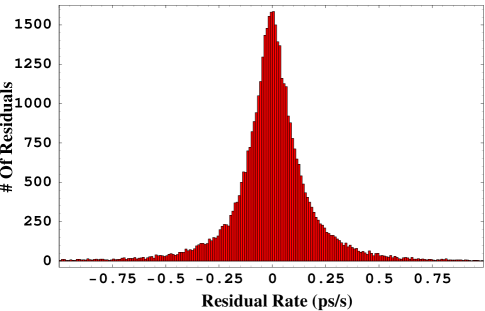
Figure 2: Distribution of the residual delay rates for all the baselines, sources, and scans of our observations.

We apply this algorithm to all scans in our observations. Actually, to ease the work, for consecutive scans of the same source, we apply the corrections found in the previous scan before performing the ambiguity check. We have tested this “automatic connector” with synthetic data for different scenarios and have obtained excellent results. An example scenario, with a remarkably high noise level, consists of delays equal to a random number of cycles (up to 5) added to randomly selected baselines every random number of scans (with an average of 50 scans between random cycles) in a dataset of 1000 scans and 10 antennas. Under such circumstances, the automatic connector finds all the random baseline-dependent cycles without introducing changes in the antenna-based overall constant cycles (see below). We repeated this test several times (with a different number of antennas and even in worse noise conditions) and the connector never introduced changes in the antenna-based overall cycles.

3.2 Antenna-based ambiguities

The antenna-based ambiguities are offsets of the phase delay, consisting of a given integer number of phase delay cycles that depend on each antenna and source. These ambiguities do not affect the phase closures and, thus, are completely transparent to the automatic connection algorithm described above. These antenna-based cycles appear very clearly in the residuals of the differenced delay observables, but can also be detected in the undifferenced residuals. To correct these antenna-based ambiguities, we applied another algorithm based on a smoothness criterion, which analyses variations between differenced (and also undifferenced) residuals of neighbouring scans that are, in modulus, close to, or larger than, a phase cycle. For each scan, the algorithm

1. finds these variations.

2. analyses whether these jumps have an antenna-based structure.

3. corrects the antenna-based phase cycle in the observations.

This algorithm was applied in a “bootstrapping” manner, i. e., beginning with a subset of 3 close-by antennas (Kitt Peak, Pie Town, and Los Alamos) and adding more antennas (one at a time) when all the residuals of the subset of antennas were finally smoothed. We show an example of one iteration of this smoothness criterion algorithm in Fig. 3.

Figure 3: Example of the effect of an antenna-dependent unmodelled phase cycle in the differenced observables associated to some baselines and source pairs (see source codes in Table 2). The baseline and source pair corresponding to each figure are indicated in the upper-left corner (BR refers to Brewster, OV to Owens Valley, and NL to North Liberty). The dashed lines represent the delays $\pm$0.06515 ns, corresponding to $+1$ and $-1$ cycle of phase at the observing frequency. The smoothness criterion algorithm (see Sect. 3.2) infers, from (a) and (b), that source 04 is the one affected by the unmodelled phase cycle and, from (c), that the affected antenna is OV; (d) corroborates the deductions extracted from the other figures.

3.3 Overall (source-based) ambiguities

Since we had phase-connected the data for each source independently, we still had to determine, for each antenna, the overall source-based ambiguity, that is, the integer number of phase cycles by which the phase delay of one source is offset from the others. This offset cannot be totally absorbed by atmospheric, clock, or astrometric corrections, and it can notably affect the astrometric results at our precision level.

We determined the overall ambiguities by again following an iterative process: first, we estimated the overall ambiguities in our weighted least-square fit. The overall ambiguities closest to an integer number of cycles of phase delay were set to be exactly equal to that integer number of cycles of phase delay. Then, we repeated the astrometric fit to obtain new estimates of the remaining overall ambiguities. Progressively, all the ambiguities were fixed to integer numbers of cycles of phase delay. For the complete set of overall ambiguities, the maximum deviation with respect to an integer number of cycles turned out to be less than one fourth of a cycle of phase delay (in fact, 40% of all the overall ambiguities deviated less than one tenth from their closest phase cycle integers).

3.4 Differenced observables in the global fit

The use of differenced observables corresponding to a given pair of sources will increase the precision in the determination of the relative positions of such pair (i. e., the position of one of the sources with respect to the position of the other). Differenced observables for a total of 24 source pairs (see Table 3) could be computed. This “network” of differenced observations introduces redundancies for sources that appear in more than one pair. These constraints in the degrees of freedom for the positions allow for an increase in the precision, not only of the relative source positions, but also of their absolute coordinates, although to a lower degree. The advantage of the redundancy introduced by the network of differenced observations can only be used when more than one pair of sources is available. Thus, the use of all our data in a unique fit provides more robust results than the sub-division of the observations in individual sets of source pairs fitted separately.

Unlike other differenced analyses, in which one source of the pairs was always fixed in the fit, in our global scheme we have differenced observables constructed with pairs of sources whose coordinates are being simultaneously estimated in the astrometric fit (except the coordinates of source 04, which are kept fixed in the fit). This led us to reconsider (see Appendix A) the concept of “changes in the relative position” of a pair of sources $(a,b)$, which is now defined as

$$\left\{\begin{array}[]{rl}\Delta\alpha^{rel}_{a}&=\Delta\alpha_{b}-\Delta\alpha_{a}-\Delta\delta_{a}\sin(\alpha_{b}-\alpha_{a})\tan(\delta_{b})\\ \Delta\delta^{rel}_{a}&=\Delta\delta_{b}-\Delta\delta_{a}\cos(\alpha_{b}-\alpha_{a})\end{array}\right.,$$ (1)

where $(\Delta\alpha^{rel}_{a},\Delta\delta^{rel}_{a})$ is the change in the relative position of source $b$ with respect to source $a$, $(\alpha_{a},\delta_{a})$ and $(\alpha_{b},\delta_{b})$ are the ICRF-Ext.2 right ascensions and declinations of sources $a$ and $b$, respectively, and $(\Delta\alpha_{a},\Delta\delta_{a})$ and $(\Delta\alpha_{b},\Delta\delta_{b})$ are the astrometric corrections for sources $a$ and $b$ resulting from our fit. These expressions have been obtained considering the curvature of the celestial sphere when none of the two sources is kept fixed in our fit. See Appendix A for more details. We notice, in particular, that $\Delta\alpha^{rel}_{b}$ and $\Delta\delta^{rel}_{b}$ need not be the negative of $\Delta\alpha^{rel}_{a}$ and $\Delta\delta^{rel}_{a}$, respectively, since the different orientations of the sources in the sky will produce a combination of their respective changes in right ascension and declination. This is particularly true for the sources close to the celestial pole, as it is the case for the high-declination sources of the S5 polar cap sample.

3.5 Global phase delay astrometric fit

We use both differenced and undifferenced observations in the same (global) fit, and the latter are included for the fit to remain sensitive to antenna-dependent parameters (i. e., clock drifts and zenith delays). We scale the standard deviations of the differenced and undifferenced phase delays separately in such a way that, for each type of data and for each baseline and source, the rms of the postfit residuals is unity. The ratio between standard deviations of the differenced and undifferenced observations is $\sim$0.67.

To estimate the astrometric uncertainties, we allowed for variations in the site coordinates, the coordinates of the Earth’s pole, and UT1$-$UTC in an auxiliary fit, but with their adjustments constrained by their a priori values and their standard deviations (see Table 1) through the use of an a priori covariance matrix. We then used the final covariance matrix of this auxiliary fit to estimate the final astrometric uncertainties, which now include all the contributions and correlations between the parameters of the geometry of the interferometer and the propagation medium. We also scaled the uncertainties of all the fitted parameters to make the reduced $\chi^{2}$ equal to unity.

Regarding the tropospheric zenith delays, the standard deviations of the fitted nodes of the piece-wise linear functions of our model were $\sim$0.01 ns. These are smaller than the expected uncertainties due to random variations in the wet component of the tropospheric delay at each site ($\sim$0.1 ns between nodes; Treuhaft & Lanyi Treuhaft1987 (1987)). These a priori, extra random variations are not contemplated in the computation of our astrometric uncertainties, because such unmodelled variations constitute a large fraction of the final rms (see figure 4), which indirectly affects the astrometric uncertainties after their scaling to obtain a reduced $\chi^{2}$ equal to unity.

Table 1: Fixed parameters in our astrometric fit and their uncertainties, according to IERS.

Fixed parameter	A-priori uncertainty
0454+844 position	300 $\mu$as (in $\alpha$ and $\delta$)
Earth Pole	0.7 mas (in $\alpha$ and $\delta$)
Site Coordinates	2 cm in each coordinate (x,y,z)
UT1 $-$ UTC	0.04 ms

Our global astrometric fit provides the standard deviations of the absolute positions of the sources. Given that we use Eq. 1 to calculate the changes in the relative positions of the sources, the corresponding standard deviations for these changes are given by the following expression:

$$\left\{\begin{array}[]{rl}\sigma(\Delta\alpha^{rel}_{a})&=\sqrt{\sum_{i,j}^{4}{\frac{\partial\Delta\alpha^{rel}_{a}}{\partial x_{i}}\frac{\partial\Delta\alpha^{rel}_{a}}{\partial x_{j}}C(x_{i},x_{j})}}\\ \sigma(\Delta\delta^{rel}_{a})&=\sqrt{\sum_{i,j}^{4}{\frac{\partial\Delta\delta^{rel}_{a}}{\partial x_{i}}\frac{\partial\Delta\delta^{rel}_{a}}{\partial x_{j}}C(x_{i},x_{j})}}\end{array}\right.,$$

where $x_{i}$ is the set of corrections $(\Delta\alpha_{b},\Delta\delta_{b},\Delta\alpha_{a},\Delta\delta_{a})$, and $C(x_{i},x_{j})$ is the element $(i,j)$ of the covariance matrix.

We tested the robustness of our astrometric results by repeating the fit with different reference sources. The new absolute source positions were compatible with those from the first fit at 1 $\sigma$ level. The relative source positions were compatible at 2 $\sigma$ level.

4 Results and discussion

We present the results of our astrometric analysis in Tables 2 and 3. Table 2 shows the astrometric corrections and corresponding uncertainties to the absolute source positions given by ICRF-Ext.2. Table 3 shows: i) the changes in the relative coordinates of the 24 source pairs, computed using Eq. 1; ii) the angular separations of the source pairs, computed from their ICRF-Ext.2 coordinates; and iii) our estimated corrections to the source pair angular separations.

As an example of the quality of our fit, we show in Fig. 4 the residuals of the undifferenced and differenced phase delays corresponding to all the observed sources and one of the longest baselines (Hancock $-$ Kitt Peak). Note the cancellation of systematic effects in the differenced data, which are still noticeable in the undifferenced data (probably unmodelled atmospheric effects). The rms of the undifferenced delays for all sources and baselines range between 55 ps (baseline Fort Davis $-$ North Liberty observing the source 02) and 6 ps (baseline Kitt Peak $-$ Pie Town observing the source 00). The rms of the differenced delays range from 35 ps (baseline Hancock $-$ Owens Valley observing the pair 11-04) to 2.2 ps (baseline Brewster $-$ Los Alamos observing the pair 18-17). The latter rms is somewhat smaller.

Figure 4: Postfit residuals of the undifferenced (above) and differenced (below) phase delays of all the pairs of sources for the baseline Hancock $-$ Kitt Peak. The dashed lines below represent the delays $\pm$0.06515 ns, corresponding to $+1$ and $-1$ cycle of phase.

We emphasise that the relative coordinates of each pair in Table 3 are not the simple subtractions of the absolute coordinates of the sources forming such a pair in Table 2 (except for those pairs with reference to the source 04; see Eq. 1). Also, the uncertainties in the relative coordinates are much smaller than those of the absolute coordinates. This is a consequence of, first, the natural cancellation of systematic errors in the differenced observables and, second, the correlations between the absolute positions estimated in the fit that account for all posible global shifts of the sources of each pair.

Figure 5: Uncertainties in the relative coordinates $\alpha$ (triangles) and $\delta$ (squares) of all the pairs of sources as a function of their separations.

Figure 6: Uncertainties in the separations of all the pairs of sources as a function of such separations. Since the behavior of the uncertainties is roughly linear, the relative errors of the separations of the sources are similar, $\sim$$3\times 10^{-9}$.

As could be expected, the standard deviations of the absolute positions are roughly the same for all sources; however, since we are using differenced observables in our fit, the standard deviations of the relative positions of the 24 pairs are strongly dependent on the separation of the sources that form the pairs. This effect can be clearly seen in Figs. 5 and 6. Figure 5 shows the uncertainties in the relative $\alpha$ and $\delta$ for the 24 pairs as a function of their separations. This behaviour is roughly linear, as predicted by the empirical formulae given by Shapiro et al. (Shapiro1979 (1979)) and corroborated by simulations of astrometric VLBA observations performed by Pradel, Charlot & Lestrade (Pradel2006 (2006)). This linearity is more clearly seen in Fig. 6, which shows the uncertainties of the estimates of the separations as a function of such separations. However, our astrometric uncertainties are $\sim$10 times smaller than those predicted by Shapiro et al. (Shapiro1979 (1979)) and those estimated by Pradel, Charlot & Lestrade (Pradel2006 (2006)) from their simulations, for typical declinations of the S5 polar cap sample sources. This improvement in precision is probably due to the fact that we have analysed the 13 sources simultaneously, instead of using the usual two-source (target/reference) scheme. Therefore, our global analysis brings more constraints on the position of the sources, which produces an immediate benefit in the precision of the astrometry for particularly high-declination sources. Moreover, unlike the phase-reference mapping technique, the tropospheric delay model is re-estimated along with the source positions in our least-square fit, which also contributes to minimise the $\chi^{2}$.

Table 2: List of the S5 polar cap sample sources.

Source	Alias	Flux density	3$\sigma$	ICRF-Ext.2 position (J2000.0)		Astrometric corrections
		(mJy)	(mJy/beam)	$\alpha$	$\delta$	$\Delta\alpha$ ($\mu$as)	$\Delta\delta$ ($\mu$as)
0016+731	00	823.1	0.5	00${}^{\textrm{h}}$ 19${}^{\textrm{m}}$ 45.786421${}^{\textrm{s}}$	73∘ 27′ 30.01750′′	$-$820 $\pm$ 320	$-$560 $\pm$ 200
0153+744	01	339.7	0.7	01${}^{\textrm{h}}$ 57${}^{\textrm{m}}$ 34.964908${}^{\textrm{s}}$	74∘ 42′ 43.22998′′	$-$150 $\pm$ 300	$-$810 $\pm$ 180
0212+735	02	2519.1	1.2	02${}^{\textrm{h}}$ 17${}^{\textrm{m}}$ 30.813373${}^{\textrm{s}}$	73∘ 49′ 32.62179′′	$-$620 $\pm$ 310	$-$280 $\pm$ 190
0454+844	04	225.3	0.6	05${}^{\textrm{h}}$ 08${}^{\textrm{m}}$ 42.363503${}^{\textrm{s}}$	84∘ 32′ 04.54402′′	0 $\pm$ 300	0 $\pm$ 300
0615+820	06	445.7	0.7	06${}^{\textrm{h}}$ 26${}^{\textrm{m}}$ 03.006188${}^{\textrm{s}}$	82∘ 02′ 25.56764′′	110 $\pm$ 160	200 $\pm$ 100
0716+714	07	1063.4	0.8	07${}^{\textrm{h}}$ 21${}^{\textrm{m}}$ 53.448459${}^{\textrm{s}}$	71∘ 20′ 36.36339′′	220 $\pm$ 360	$-$100 $\pm$ 210
0836+710	08	1772.9	0.8	08${}^{\textrm{h}}$ 41${}^{\textrm{m}}$ 24.365262${}^{\textrm{s}}$	70∘ 53′ 42.17301′′	280 $\pm$ 360	$-$400 $\pm$ 220
1039+811	10	848.4	1.0	10${}^{\textrm{h}}$ 44${}^{\textrm{m}}$ 23.062554${}^{\textrm{s}}$	80∘ 54′ 39.44303′′	660 $\pm$ 190	$-$30 $\pm$ 110
1150+812	11	988.3	1.0	11${}^{\textrm{h}}$ 53${}^{\textrm{m}}$ 12.499130${}^{\textrm{s}}$	80∘ 58′ 29.15451′′	$-$450 $\pm$ 180	$-$640 $\pm$ 120
1749+701	17	468.7	0.8	17${}^{\textrm{h}}$ 48${}^{\textrm{m}}$ 32.840231${}^{\textrm{s}}$	70∘ 05′ 50.76882′′	460 $\pm$ 380	140 $\pm$ 230
1803+784	18	2334.5	0.7	18${}^{\textrm{h}}$ 00${}^{\textrm{m}}$ 45.683914${}^{\textrm{s}}$	78∘ 28′ 04.01849′′	70 $\pm$ 230	130 $\pm$ 140
1928+738	19	3088.6	1.1	19${}^{\textrm{h}}$ 27${}^{\textrm{m}}$ 48.495167${}^{\textrm{s}}$	73∘ 58′ 01.57010′′	90 $\pm$ 310	0 $\pm$ 190
2007+777	20	1271.0	0.5	20${}^{\textrm{h}}$ 05${}^{\textrm{m}}$ 30.998511${}^{\textrm{s}}$	77∘ 52′ 43.24763′′	400 $\pm$ 240	$-$250 $\pm$ 150

Table 3: Astrometric results for all the observed source pairs.

Source pair	Change in the relative coordinates		ICRF-Ext.2 angular separation	Correction to angular separation
	$\Delta\alpha^{rel}$ ($\mu$as)	$\Delta\delta^{rel}$ ($\mu$as)	(deg)	$\mu$as
01-00	$-$990 $\pm$ 70	180 $\pm$ 40	6.770731378	850 $\pm$ 70
01-02	$-$390 $\pm$ 16	520 $\pm$ 14	1.614936659	$-$620 $\pm$ 20
04-01	$-$150 $\pm$ 110	$-$810 $\pm$ 140	12.284604495	810 $\pm$ 140
04-02	$-$620 $\pm$ 110	$-$280 $\pm$ 140	12.703755162	450 $\pm$ 140
04-06	110 $\pm$ 40	200 $\pm$ 40	3.332785200	$-$110 $\pm$ 40
04-07	220 $\pm$ 150	$-$100 $\pm$ 160	14.393224831	150 $\pm$ 170
04-10	660 $\pm$ 100	$-$30 $\pm$ 110	10.085113231	390 $\pm$ 120
06-07	$-$80 $\pm$ 90	$-$300 $\pm$ 120	11.093608166	280 $\pm$ 130
06-10	350 $\pm$ 90	$-$120 $\pm$ 80	9.134095175	350 $\pm$ 100
08-04	$-$400 $\pm$ 180	240 $\pm$ 80	16.400909237	460 $\pm$ 190
08-07	$-$180 $\pm$ 70	270 $\pm$ 20	6.419140221	150 $\pm$ 70
08-10	730 $\pm$ 110	310 $\pm$ 90	12.179115583	760 $\pm$ 140
11-04	$-$350 $\pm$ 120	$-$120 $\pm$ 100	11.407147545	350 $\pm$ 140
11-10	930 $\pm$ 40	580 $\pm$ 20	2.699376639	$-$1020 $\pm$ 30
11-18	1280 $\pm$ 130	110 $\pm$ 140	14.839207812	700 $\pm$ 170
11-20	1530 $\pm$ 130	$-$600 $\pm$ 200	18.626089045	1180 $\pm$ 210
18-00	$-$1050 $\pm$ 160	$-$550 $\pm$ 200	20.844902015	$-$140 $\pm$ 240
18-04	$-$60 $\pm$ 80	130 $\pm$ 190	16.901504141	$-$140 $\pm$ 190
18-17	340 $\pm$ 50	10 $\pm$ 100	8.408293010	$-$30 $\pm$ 100
18-20	260 $\pm$ 70	$-$360 $\pm$ 40	6.342305345	370 $\pm$ 70
19-17	350 $\pm$ 70	140 $\pm$ 70	8.491093690	$-$360 $\pm$ 90
19-20	330 $\pm$ 30	$-$250 $\pm$ 50	4.521891420	$-$15 $\pm$ 50
20-00	$-$1150 $\pm$ 130	$-$450 $\pm$ 140	15.450912042	$-$500 $\pm$ 180
20-02	$-$910 $\pm$ 150	$-$300 $\pm$ 200	20.618479511	$-$300 $\pm$ 240

4.1 Brief discussion of some selected sources

All the astrometric corrections shown in Tables 2 and 3 are corrections to the ICRF-Ext.2 positions. These ICRF-Ext.2 positions, determined using the group delay observable obtained from dual frequency observations at 8.4 & 2.3 GHz, are not directly comparable to our 15.4 GHz phase delay position estimates: first, the ICRF-Ext.2 positions are not defined with respect to any specific phase centre on the source maps, which our positions are; second, even if the source structure is not astrometrically significant, source opacity effects could be present while comparing the source positions determined at 8.4, 2.3, and 15.4 GHz.

From Table 2, we can calculate mean corrections to the ICRF-Ext.2 coordinates. We find mean corrections of 278 and 170 $\mu$as in right ascension and declination, respectively. Our values are similar to those found by Jacobs et al. (Jacobs2004 (2004)). These authors are pursuing the extension of the ICRF-Ext.2 to 24 (K-band) and 43 GHz (Q-band). From VLBA global observations they found an agreement between the X/S-frame and K-band frame to within 330 and 590 $\mu$as in right ascension and declination, respectively, comparable to our mean corrections.

Structure effects must contribute to the corrections of the separations of the source pairs given in Table 3. Only seven out of the thirteen S5 sources are defining ICRF-Ext.2 sources and only one of them (source 07) is unresolved (following the definition used by Charlot Charlot1990 (1990)) at X-band. Actually, a detailed look at the structure of the radio sources can provide some hints to explain the relatively large corrections in the last column of Table 3. For instance, pairs with source 01 as member, which has an X-band structure index of 4 (very extended, see Charlot Charlot1990 (1990)) show large corrections to the ICRF-Ext.2 coordinates; likewise, the corrections corresponding to pairs containing source 11 can be explained in terms of a southwest bending of the jet near the core (see maps in Paper I & II). However, a detailed interpretation of the astrometric information obtained by comparing with the results from other epochs and frequencies in our astrometric project is beyond the scope of this paper and will be published elsewhere.

5 Conclusions

We report here on the first high-precision, wide-field astrometric results at 15.4 GHz of our multi-frequency monitoring of the S5 polar cap sample. To obtain those results we first developed the package uvpap, an extensively improved version of the vlbi3 program (Robertson Robertson1975 (1975)). The ability of uvpap to use differenced phase delays, along with newly developed phase-connection algorithms, enables us the use of differenced phase delays in global astrometric observations. We discuss the impact of the differenced phase delays on our global astrometric analysis and show that their use increases the precision of the relative source positions by a factor of $\sim$10 compared with the precision achievable using the phase-reference technique with a pair of sources (Pradel, Charlot & Lestrade Pradel2006 (2006)). The astrometric precisions obtained linearly decrease (from 14 to 200 $\mu$as) as the separations between the sources increase (from $\sim$1.6 to $\sim$20.8 degrees), with the result that the fractional errors in determining the separations of all the studied source pairs are similar ($\sim$3$\times 10^{-9}$).

We obtain some large corrections for the relative coordinates and separations of the sources. From all the 24 pairs studied, 10 have separation corrections above 500 $\mu$as and, of those, 4 have corrections above 900 $\mu$as. These corrections could be caused by opacity effects (our observations are at 15.4 GHz, and the ICRF-Ext.2 positions are based on 8.4 and 2.3 GHz observations) and by source structure effects (we are relating our astrometric positions to the phase centres of the source maps, that is, the peaks of brightness; the ICRF-Ext.2 positions are not well-defined on the source structures). Other wide-field, high-precision astrometric analyses of these sources at other frequencies and other epochs are currently under way. This multi-epoch and multi-frequency study will eventually provide spectral information and the absolute kinematics for all sources in the sample. Ultimately, we expect to provide a definitive test of the stationarity of the innermost radio-source cores, associated to the massive black holes, which is a basic tenet of the standard jet interaction model (Blandford & Königl Blandford1979 (1979)). In addition, our results will be an excellent complement to future $\mu$as-precise astrometry at optical wavelengths.

Appendix A Relative position changes for free-moving sources in the sky

Let $\alpha_{a}$ and $\delta_{a}$ be the right ascension and declination of source $a$, and $\alpha_{b}$ and $\delta_{b}$ the right ascension and declination of source $b$. Then, the relative position of source $b$ with respect to $a$ is

$$\alpha^{rel}_{a}=\alpha_{b}-\alpha_{a}$$ (2)

$$\delta^{rel}_{a}=\delta_{b}-\delta_{a}.$$

In the simple case that one of the two sources (the reference source $a$) is kept fixed in the sky, the change in the relative position between this pair of sources can be well defined from equations (A.1):

$$\left\{\begin{array}[]{rl}\Delta\alpha^{rel}_{a}=\Delta\alpha_{b}\\ \Delta\delta^{rel}_{a}=\Delta\delta_{b}\end{array}\right.,$$ (3)

where $a$ is the reference (fixed) source and $b$ the target (free) source; $\Delta\alpha_{b}$ and $\Delta\delta_{b}$ are the corrections to the position of source $b$, maintaining the source $a$ fixed in the fit. However, Eqs. (A.1) are not appropriate when the two sources can change their positions in the fit, since the curvature of the celestial coordinate system affects the robustness of Eqs. (A.1) under a global shift of the source pair. To illustrate with a simple example for two sources separated by 12 hours in right ascension, a global shift, $\epsilon$, in declination would originate a change of $2\epsilon$ in the relative declination of these sources, according to (A.1). (The declinations of these sources will change with opposite signs.) The relative coordinates between this pair of sources would, then, appear to change dramatically under a global shift of the pair. In other words, we need to define a reference point in the sky to measure the shift of $b$ with respect to $a$. In our analysis, for each pair of sources, we select the nominal position of the reference source as the reference point for the study of that particular pair. In practice, such a selection is equivalent to applying a global rotation $\Re$ in such a way that the source $a$ is rotated back to its initial (i. e. nominal) position. According to this rotation, the change in the coordinates of source $a$ is

$$\Re\Rightarrow\left\{\begin{array}[]{rl}\alpha_{a}+\Delta\alpha_{a}&\rightarrow\alpha_{a}\\ \delta_{a}+\Delta\delta_{a}&\rightarrow\delta_{a}\end{array}\right.,$$ (4)

where $\Delta\alpha_{a}$ and $\Delta\delta_{a}$ are the corrections to the right ascension and declination of source $a$. This rotation, $\Re$, will have the corresponding effect on the coordinates of source $b$, which are

$$\Re\Rightarrow\left\{\begin{array}[]{rl}\alpha_{b}+\Delta\alpha_{b}&\rightarrow\alpha_{b}+\Delta\alpha^{m}_{ab}+\Delta\alpha_{b}\\ \delta_{b}+\Delta\delta_{b}&\rightarrow\delta_{b}+\Delta\delta^{m}_{ab}+\Delta\delta_{b}\end{array}\right.,$$ (5)

where $\Delta\alpha^{m}_{ab}$ and $\Delta\delta^{m}_{ab}$ are the changes in right ascension and declination that the rotation $\Re$ causes on the position of source $b$. Thus, the change in the relative coordinates of $b$ with respect to $a$ will be

$$\left\{\begin{array}[]{rl}\Delta\alpha^{rel}_{a}=\Delta\alpha_{b}+\Delta\alpha^{m}_{ab}\\ \Delta\delta^{rel}_{a}=\Delta\delta_{b}+\Delta\delta^{m}_{ab}\end{array}\right..$$ (6)

When the coordinates of both sources, $a$ and $b$, are corrected in the astrometric fit, we must use these equations instead of Eq. 3.

Figure 7: Graphic representation of the rotation $\Re$ that we apply to sources $a$ and $b$. In (a.1), the coordinates of both sources, $a$ and $b$, have been corrected an amount $\@vec{{\Delta}a}=(\Delta\alpha_{a},\Delta\delta_{a})$ and $\@vec{{\Delta}b}=(\Delta\alpha_{b},\Delta\delta_{b})$, respectively. In (a.2), we apply a rotation $\Re$ that brings source $a$ back to its ICRF position (maintaining $P_{ang}$ constant) and causes the shift $\@vec{{\Delta}^{m}_{ab}}=(\Delta\alpha^{m}_{ab},\Delta\delta^{m}_{ab})$ on source $b$. The total shift of $b$ will therefore be the addition of the corrections $\@vec{{\Delta}b}$ and $\@vec{{\Delta}^{m}_{ab}}$.

From all possible rotations $\Re$ in the sky that move the source $a$ back to its nominal position, we selected the one that causes the direction of the arc between $a$ and $b$ (i. e., the position angle of $b$ with respect to $a$) to remain unchanged. According to the sine theorem (see Fig. 7):

$$\cos{\delta_{b}}\sin{(\alpha_{a}-\alpha_{b})}=\sin{\lambda}\sin{P_{ang}}$$ (7)

where $\lambda$ is the arclength between $a$ and $b$, and $P_{ang}$ is the position angle of $b$ with respect to $a$. In our case, this can be expressed as

$$\cos{(\delta_{b}+\Delta\delta_{b})}\sin{(\alpha_{b}-\alpha_{a}+\Delta\alpha_{b}-\Delta\alpha_{a})}=$$

$$\cos{(\delta_{b}+\Delta\delta^{m}_{ab}+\Delta\delta_{b})}\sin{(\alpha_{b}-\alpha_{a}+\Delta\alpha^{m}_{ab}+\Delta\alpha_{b})},$$ (8)

For a first-order approximation of the astrometric corrections ($\sim$0.5 mas, see Table 2), the condition 8, together with the constancy of the arclength between $a$ and $b$ under the rotation $\Re$, is satisfied if, and only if

$$\Delta\alpha^{m}_{ab} = -\Delta\alpha_{a}-\Delta\delta_{a}\sin(\alpha_{b}-\alpha_{a})\tan(\delta_{b})$$ (9)

$$\Delta\delta^{m}_{ab} = -\Delta\delta_{a}\cos(\alpha_{b}-\alpha_{a}).$$

When we apply these relationships to Eq. 6, we obtain Eq. 1 of this paper directly:

$$\Delta\alpha^{rel}_{a} = \Delta\alpha_{b}-\Delta\alpha_{a}-\Delta\delta_{a}\sin(\alpha_{b}-\alpha_{a})\tan(\delta_{b})$$ (10)

$$\Delta\delta^{rel}_{a} = \Delta\delta_{b}-\Delta\delta_{a}\cos(\alpha_{b}-\alpha_{a}).$$