Goldstone modes and electromagnon fluctuations in the conical cycloid state of a multiferroic

Abstract

Using a phenomenological Ginzburg-Landau theory for the magnetic conical cycloid state of a multiferroic, which has been recently reported in the cubic spinel CoCr₂O₄, we discuss its low-energy fluctuation spectrum. We identify the Goldstone modes of the conical cycloidal order, and deduce their dispersion relations whose signature anisotropy in momentum space reflects the symmetries broken by the ordered state. We discuss the soft polarization fluctuations, the ‘electromagnons’, associated with these magnetic modes and make several experimental predictions which can be tested in neutron scattering and optical experiments.

I Introduction

Although ferromagnetism and antiferromagnetism are the two most widely studied forms of magnetic order, more complicated, spatially modulated magnetic order parameters are also important and interesting from both fundamental and technological perspectives. A salient example, which occurs in the new class of ‘multiferroics’ Fiebig ; Ramesh ; Tokura1 ; Cheong – materials that display an amazing coexistence and interplay of long range magnetic and ferroelectric orders – is magnetic transverse helical, or ‘cycloidal’, order. This order has acquired prominence Tokura1 ; Cheong ; Katsura1 ; Mostovoy ; Lawes ; Tokura2 ; Cheong2 ; Chapon ; Goto ; Kenzelmann ; Pimenov ; Sneff ; Tokura3 ; Tokura4 ; Dagotto ; Katsura2 since it can induce, via broken spatial inversion symmetry Mostovoy ; Lawes , a concomitant electric polarization ($\mathbf{P}$) in a class of ternary oxides, leading to interesting physics of competing and colluding ordering phenomena as well as potential applications Fiebig ; Ramesh ; Tokura1 ; Cheong . Among the exciting class of multiferroic materials, the cubic spinel oxide CoCr₂O₄ is even more unusual, since it displays not only the coexistence of $\mathbf{P}$ with a spatially modulated magnetic order, but also with a uniform magnetization ($\mathbf{M}$) Tokura4 in a so-called ‘conical cycloid’ state (see below).

Since in the conical cycloid state, the long range magnetic and polar orders are intertwined, it is crucial to understand the associated soft modes (i.e., low energy collective excitations), which should also be ‘hybridized’, leading to intriguing potential applications based on the electronic excitation of spin waves Khitun and vice versa. A second motivation for studying the soft collective mode spectrum of a system with a complicated set of order parameters, such as the conical cycloid state, is that the Goldstone modes themselves caricature the underlying pattern of the broken symmetries, and thus, strengthen the understanding of the ordered state itself. In this paper, we do this by first identifying the magnetic Goldstone modes (i.e., magnons or spin waves) of the conical cycloidal order and deducing their dispersion relations which, as we clarify, simply reflect the complex, anisotropic pattern of the underlying broken symmetries. We make several predictions for inelastic neutron scattering experiments based on our results for the magnetic fluctuations. We then identify the associated soft polarization fluctuations, which constitute a dielectric manifestation of the magnetic modes, ‘electromagnons’, which can be observed in optical experiments. The interesting interplay of magnons and electromagnons in cubic multiferroics is the topic of this paper.

CoCr₂O₄, with the lattice structure of a cubic spinel, enters into a state with a uniform magnetization at a temperature $T_{m}=93$ K. Microscopically, the magnetization is of ferrimagnetic origin Tokura4 , and in what follows we will only consider the ferromagnetic component, $\mathbf{M}$, of the magnetization of a ferrimagnet. At a lower critical temperature, $T_{c}=26$ K, the system develops a spacial helical modulation of the magnetization in a plane transverse to the large uniform component. Such a state, for general helicoidal modulation transverse to the uniform magnetization, can be described by an order parameter,

$$\mathbf{M}_{h}=m_{1}\hat{e}_{1}\cos(\mathbf{q}\cdot\mathbf{r})+m_{2}\hat{e}_{2}\sin(\mathbf{q}\cdot\mathbf{r})+m_{3}\hat{e}_{3},$$ (1)

where $\{\hat{e}_{i}\}$ form an orthonormal triad. When the pitch vector, $\mathbf{q}$, is normal to the plane of the rotating components, the rotating components form a conventional helix Belitz . A more complicated modulation arises when $\mathbf{q}$ lies in the plane of the rotating components. For $m_{3}=0$, we will call such a state, which has been recently observed in a number of multiferroic ternary oxides Tokura1 ; Cheong ; Lawes ; Tokura2 ; Cheong2 ; Chapon ; Goto ; Kenzelmann ; Pimenov ; Sneff ; Tokura3 , an ‘ordinary cycloid’ state because the profile of the magnetization resembles the shape of a cycloid. The cycloid state with $m_{3}\neq 0$ will be called a ‘conical cycloid’ state, because the tip of the magnetization falls on the edge of a cone, see Fig. 1. This is the low temperature magnetic ground state in CoCr₂O₄, and is responsible for its many unusual properties, for e.g., the ability to tune $\mathbf{P}$ via tuning the uniform piece of the magnetization by a small magnetic field $\sim 0.5$ T Tokura4 . Notice that these states break the spin rotational and the coordinate space rotational, translational and inversion symmetries. It is easy to visualize that the helical, but not the cycloidal, modulation preserves a residual coordinate space $U(1)$ symmetry (followed by a translation) about the pitch vector.

II Intuitive understanding of the Goldstone modes

To gain an intuitive understanding of the Goldstone modes, let’s first consider the broken symmetries of the conical cycloid state, with a representative mean-field order parameter,

$$M_{c}(\mathbf{r})=(m_{1}\cos(qx),m_{2}\sin(qx),m_{3}),$$ (2)

shown in Fig. 1. As mentioned above, this state breaks the spin space rotation and the coordinate space rotation and translation symmetries. Note, however, that the translation symmetry is broken only in the direction of $\mathbf{q}$. Since translational symmetry is spontaneously broken in this system, uniform translations along the direction of ${\mathbf{q}}$, which can be parameterized by the phase fluctuation $\varphi(\mathbf{r})$, where the fluctuating magnetization may be given by $\mathbf{M}(\mathbf{r})=(m_{1}\cos(qx+\varphi(\mathbf{r})),m_{2}\sin(qx+\varphi(\mathbf{r})),m_{3})$, must be a Goldstone mode. It is important to realize, however, that the elastic energy for this fluctuation cannot involve $(\partial_{y}\varphi)^{2},(\partial_{z}\varphi)^{2}$, while it must involve the longitudinal component, $(\partial_{x}\varphi)^{2}$. This is because a uniform rotation of $\mathbf{q}$, $\varphi(\mathbf{r})=\alpha y+\beta z$, rotating the pitch vector from ($q,0,0$) to ($q,\alpha,\beta$) must not cost any energy since the underlying Hamiltonian is assumed to be rotationally invariant. The elastic energy must include $(\partial_{x}\varphi)^{2}$, however, since a change of the magnitude of $\mathbf{q}$ does cost energy. Thus, in momentum space, the dispersion relation for this Goldstone mode should be much softer in the directions transverse to $\mathbf{q}$ than in the longitudinal direction.

The absence of a residual symmetry about $\mathbf{q}$ gives rise to a second Goldstone mode in the conical cycloid state. Notice that a uniform rotation of the cycloidal plane and the uniform magnetization about $\hat{\mathbf{q}}$ does not cost energy, and therefore, such a rotation at long wavelengths must cost vanishing energy. In the conventional helical state, this mode is already contained in the phase $\varphi$, since a uniform translation of a circular helix long its pitch axis (i.e., a uniform $\varphi$) is equivalent to a rotation about the pitch axis by $\varphi$. The Goldstone mode fluctuations in the conical cycloid state are depicted pictorially in Fig. 2.

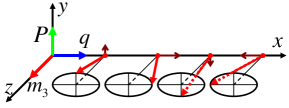
Figure 1: (Color online) The conical cycloid state with the mean field order parameter given in Eq. 2. The spins rotate along the pitch vector, $\mathbf{q}$, on the cycloidal ($x-y$) plane. The uniform component, $m_{3}$, which is along the $\hat{z}$ direction makes the magnetization tip fall on the edge of a cone. The polarization, $P$, is perpendicular to both $\mathbf{q}$ and the uniform magnetization.

III Ginzburg-Landau Hamiltonian

Since $\mathbf{M}$ and $\mathbf{P}$ respectively break time reversal and spatial inversion symmetry, the leading $\mathbf{P}$-dependent piece in a Ginzburg-Landau Hamiltonian density, $h_{P}$, for a centrosymmetric, time reversal invariant system with cubic symmetry is Mostovoy ,

$$h_{P}=\mathbf{P}^{2}/2\chi+\alpha\mathbf{P}\cdot\mathbf{M}\times\nabla\times\mathbf{M},$$ (3)

where $\chi>0$ and $\alpha$ are coupling constants. We assume that $\mathbf{P}$ is a slave of $\mathbf{M}$, in the sense that a non-zero $\mathbf{P}$ only occurs due to the spontaneous development of a magnetic state with a non-zero $\mathbf{M}\times\nabla\times\mathbf{M}$. We consider a full Hamiltonian that is completely invariant under simultaneous rotations of positions and magnetization. This guarantees that any phase that can occur in our model is necessarily allowed in a crystal of any symmetry. The full Hamiltonian is given by Zhang , $H=\int(h_{M}+h_{P})d\mathbf{r}\equiv\int hd\mathbf{r}$. Using $\mathbf{P=-}\chi\alpha\mathbf{M}\times\nabla\times\mathbf{M}$ to eliminate $\mathbf{P}$, we can write the total Hamiltonian density $h$ entirely in terms of $\mathbf{M}$,

$$h = t\mathbf{M}^{2}+u\mathbf{M}^{4}+K_{0}\left(\nabla\cdot\mathbf{M}\right)^{2}+K_{1}\left(\nabla\times\mathbf{M}\right)^{2}$$ (4)

$$+K_{2}\mathbf{M}^{2}\left(\nabla\cdot\mathbf{M}\right)^{2}+K_{3}\left(\mathbf{M}\cdot\nabla\times\mathbf{M}\right)^{2}$$

$$+K_{4}\left|\mathbf{M}\times\nabla\times\mathbf{M}\right|^{2}$$

$$+D_{L}|\nabla\left(\nabla\cdot\mathbf{M}\right)\mathbf{|}^{2}+D_{T}|\nabla\left(\nabla\times\mathbf{M}\right)\mathbf{|}^{2},$$

where we have $u$, $D_{L,T}>0$ for stability. Due to competing magnetic interactions, some of the $K_{i}$ can be negative.

To discuss the parameter space for the conical cycloid state, $t$ is assumed to cross zero at $T_{m}$, and the system enters into a state with a uniform magnetization $m_{3}=\sqrt{-t/2u}$. As $T$ drops further, the elliptic conical cycloid state, with the uniform magnetization normal to the cycloidal plane and $\mathbf{q}$ in the plane of the cycloid, i.e., with a representative order parameter given by Eq. 2, is the lowest energy state in the regime $t<0$, $K_{3}<0$, $K_{0}<0$, $0<K_{1}<<-K_{3}m_{3}^{2}$. In this regime, Eq. 2 defines the ground state among all the possible states with arbitrary mutual angles between the uniform magnetization, $\mathbf{q}$, and the cycloid plane. $K_{2}$, and $K_{4}$ are relatively unimportant for this state (Eq. 2 satisfies the saddle point equations with or without them), therefore, in what follows, we will set $K_{2}=K_{4}=0$ for simplicity Zhang .

IV Goldstone modes in the conical cycloid state

To identify the Goldstone modes and to calculate their correlation functions, we follow standard methods: we first write $\mathbf{M}$ as its mean-field solution (describing the conical cycloid state) plus the fluctuations. We then substitute this total $\mathbf{M}$ in the Hamiltonian, Eq. 4, and expand the Hamiltonian to the second order in the fluctuation modes. A straightforward (though tedious) diagonalization of the fluctuation piece of the Hamiltonian would then produce the fluctuation modes (eigenvectors) and their energy dispersions (eigenvalues). As we will see below, there are four fluctuation modes of the conical cycloid state, among which two are massive and the other two ($\alpha$ and $\delta_{x}$, see below) are soft (Goldstone modes) in the long wavelength limit. By inverting the fluctuation part of the Hamiltonian, one can also read-off the correlation functions of the soft modes from the matrix elements.

Te begin, we write the total magnetization as $\mathbf{M}=\mathbf{M}_{c}+\delta\mathbf{M}$, where $\delta\mathbf{M}$ describes the fluctuations above the saddle point solution $\mathbf{M}_{c}$. Generally, $\mathbf{M}$ can be written as,

$$M=\left(\begin{array}[]{c}-m_{3}\delta_{y}+m_{1}\cos\left(qx+\varphi\right)-m_{2}\delta_{z}\sin\left(qx+\varphi\right),\\ -m_{3}\delta_{x}+m_{2}\sin\left(qx+\varphi\right)+m_{1}\delta_{z}\cos\left(qx+\varphi\right),\\ m_{3}+\delta_{y}m_{1}\cos\left(qx+\varphi\right)+\delta_{x}m_{2}\sin\left(qx+\varphi\right)\end{array}\right)$$ (5)

where $\varphi$ describes the fluctuation of $\mathbf{q}$, and $\delta_{y}$ and $\delta_{z}$ describe the rotation of the cycloidal plane and $m_{3}$ about the $y$ and the $z$ axes, respectively. Note that, for the circular cycloidal state $(m_{1}=m_{2})$, $\delta_{z}$ can be taken to be zero since it only renormalizes $\varphi$ in this case. $\delta_{x}$ describes the rotation of the cycloidal plane about the pitch vector itself. Expanding $\mathbf{M}$ to first order in the fluctuation variables, we have

$$\delta\mathbf{M}=\left(\begin{array}[]{c}-m_{3}\delta_{y}-\left(\varphi m_{1}+\delta_{z}m_{2}\right)\sin qx\\ -m_{3}\delta_{x}+\left(\varphi m_{2}+\delta_{z}m_{1}\right)\cos qx\\ \delta_{y}m_{1}\cos qx+\delta_{x}m_{2}\sin qx\end{array}\right)$$ (6)

To obtain the soft modes, we expand the Hamiltonian to second order in $\delta\mathbf{M}$. It is easy to check that the coefficient of the first order term is zero from the saddle point equations. The second order gives

$$\delta H = t\left(\delta\mathbf{M}\right)^{2}+u\left[2\mathbf{M}_{c}^{2}\left(\delta\mathbf{M}\right)^{2}+4\left(\mathbf{M}_{c}\cdot\delta\mathbf{M}\right)^{2}\right]$$ (7)

$$+D_{L}|\nabla\left(\nabla\cdot\delta\mathbf{M}\right)\mathbf{|}^{2}+D_{T}|\nabla\left(\nabla\times\delta\mathbf{M}\right)\mathbf{|}^{2}$$

$$+K_{0}\left[\left(\nabla\cdot\delta\mathbf{M}\right)^{2}\right]+K_{1}\left[\left(\nabla\times\delta\mathbf{M}\right)^{2}\right]$$

$$+K_{3}\left(\delta\mathbf{M}\cdot\nabla\times\mathbf{M}_{c}+\mathbf{M}_{c}\cdot\nabla\times\delta\mathbf{M}\right)^{2}$$

$$+2K_{3}\left[\mathbf{M}_{c}\cdot\nabla\times\mathbf{M}_{c}\right]\left[\delta\mathbf{M}\cdot\nabla\times\delta\mathbf{M}\right]$$

Substituting Eq. 6 into Eq. 7, taking the Fourier transform, and denoting $\delta_{0}=\varphi$, we find, $\delta H=\sum_{\mathbf{p},i,j}\delta_{i}(-\mathbf{p})\Gamma_{ij}(\mathbf{p})\delta_{j}(\mathbf{p})$, where, $i$ and $j$ run from 0 to 3. For brevity, we omit the full form of the $4\times 4$ matrix $\Gamma$ here.

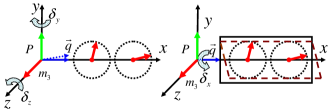
Figure 2: (Color online) Left: The magnetic Goldstone mode $\alpha$ of the conical cycloid state. For an arbitrary small fluctuation of the pitch vector, $\mathbf{q}$, the cycloidal plane and the uniform magnetization must also rotate by angles $\delta_{y}$ and $\delta_{z}$ about the axes $y$ and $z$, respectively, for a zero energy deformation. Right: The other Goldstone mode $\delta_{x}$. $\delta_{x}$ describes the rotation fluctuation of the entire system about the pitch vector, and, if spatially uniform, costs no energy. For clarity, the rotations of $m_{3}$ and $\mathbf{P}$ are not shown.

We should note, at this point, that in order for the fluctuation mode $\varphi$, and, in effect, the direction fluctuation of $\mathbf{q}$ to cost vanishing energy for infinite wavelengths, the cycloidal plane and the uniform magnetization themselves must rotate about the $y$ and the $z$ axes. The true Goldstone mode, for the third rotation fluctuation $\delta_{x}=0$, must then be a linear combination of $\varphi,\delta_{y}$ and $\delta_{z}$. To capture this soft mode, we first take $\delta_{x}=0$ and diagonalize the resulting $3\times 3$ matrix. The eigenvalues for two eigenvectors, $\beta,\gamma$, remain non-zero even when the momentum $p\rightarrow 0$ (massive modes), but the other eigenvalue becomes zero in this limit (soft mode). The corresponding eigenstate of the soft mode, to linear order in $p=|\mathbf{p}|$, is given by,

$$\alpha=\varphi\left(\mathbf{p}\right)+ip_{z}\delta_{y}\left(\mathbf{p}\right)/q+ip_{y}\delta_{z}\left(\mathbf{p}\right)/q.$$ (8)

This is one of the two cycloidal Goldstone modes found in this paper, see Fig. 2. To order $p^{2}$, we have the corresponding eigenvalue,

$$\omega_{0}=2\left(m_{1}^{2}+m_{2}^{2}\right)q^{2}p_{x}^{2}.$$ (9)

As expected, there is no contribution from $p_{y},p_{z}$ at this order. As emphasized before, this is a reflection of the rotational symmetry of the underlying Hamiltonian. The next higher order contribution to the Goldstone mode eigenvalue is given by $\omega_{1}=u_{1}p_{y}^{4}+u_{2}p_{z}^{4}+u_{3}p_{x}^{4}+u_{4}p_{x}^{2}p_{y}^{2}+u_{5}p_{y}^{2}p_{z}^{2}+u_{6}p_{x}^{2}p_{z}^{2}$, where the $u_{i}$’s are functions of $m_{1},$ $m_{2}$, $m_{3}$ and the coupling constants $K_{0}$, $K_{1}$, $K_{3},D_{L,T}$.

The other Goldstone mode of the conical cycloid state is simply the mode $\delta_{x}$, see Fig. 2, with the momentum space dispersion relation starting at the order $p_{x}^{2},p_{y}^{2},p_{z}^{2}$. As explained before, spatially uniform rotation of the whole system about the direction $\hat{\mathbf{q}}=\hat{x}$ does not cost energy, so the long wavelength fluctuations, represented by $\delta_{x}$, cost vanishing energy.

In the presence of lattice and spin anisotropies, the foregoing results are valid only above the anisotropy energies. The anisotropic dispersion of the mode $\alpha$ crosses over to a more isotropic dispersion, one which depends quadratically on all of $p_{x},p_{y},p_{z}$, below the lattice anisotropy energy. However, it continues to remain a true Goldstone mode because of the broken translational symmetry. In this respect, this cycloidal magnon is analogous to the phonon mode in a crystal, rather than a true magnon mode. Below the weak spin anisotropy energy, the other Goldstone mode, $\delta_{x}$, should acquire a gap given by this spin anisotropy energy.

In the most general case, the two soft modes will couple. In terms of the corresponding eigenstates, the $4\times 4$ matrix can be rewritten as a $2\times 2$ matrix (plus unimportant contributions coming from the massive modes),

$$\left(\begin{array}[]{cc}2\left(m_{1}^{2}+m_{2}^{2}\right)q^{2}p_{x}^{2}+\omega_{1}&-p_{x}p_{z}v_{0}-ip_{x}p_{y}p_{z}v_{1}/q\\ -p_{x}p_{z}v_{0}+ip_{x}p_{y}p_{z}v_{1}/q&f(p^{2})+m_{2}^{2}D_{T}p^{4}/2\end{array}\right)$$ (10)

where $v_{0},v_{1}$ are constants and $f(p^{2})$ is a second order polynomial function of $p_{x},p_{y},p_{z}$. By inverting this matrix, we find,

$$C_{\alpha\alpha}\left(\mathbf{p}\right) = \sum\nolimits_{i=x,y,z}\eta_{i}p_{i}^{2}/\Delta\left(\mathbf{p}\right)$$

$$C_{\delta_{x}\delta_{x}}\left(\mathbf{p}\right) = \left[4\left(g_{1}+g_{2}\right)q^{2}p_{x}^{2}+\omega_{1}\right]/\Delta\left(\mathbf{p}\right)$$

$$C_{\alpha\delta_{x}}\left(\mathbf{p}\right) = p_{x}p_{z}v_{0}/\Delta\left(\mathbf{p}\right)$$ (11)

where $C_{\mu\nu}\left(\mathbf{p}\right)=\left\langle\mu\left(-\mathbf{p}\right)\nu\left(\mathbf{p}\right)\right\rangle$, $\Delta\left(\mathbf{p}\right)=p_{x}^{2}\sum_{i=x,y,z}\beta_{i}p_{i}^{2}+\omega_{1}\sum_{i=x,y,z}\eta_{i}p_{i}^{2}+...$ is the determinant of the matrix (10), and the $\eta_{i}$’s and the $\beta_{i}$’s are constants. Remarkably, for $p_{x}=0$, we find,

$$C_{\alpha\alpha}\left(\mathbf{p}\right) = \omega_{1}^{-1}\sim\left(\sum\nolimits_{i,j=y,z}p_{i}^{2}p_{j}^{2}\right)^{-1}$$

$$C_{\delta_{x}\delta_{x}}\left(\mathbf{p}\right) \sim \left(\beta_{y}p_{y}^{2}+\beta_{z}p_{z}^{2}\right)^{-1}\sim\left(\sum\nolimits_{i=y,z}p_{i}^{2}\right)^{-1}$$

$$C_{\alpha\delta_{x}}\left(\mathbf{p}\right) = 0,$$ (12)

so there is no contribution from $p_{y}$ and $p_{z}$ to order $p^{2}$ in the $C_{\alpha\alpha}\left(\mathbf{p}\right)$ correlator, as expected.

V Magnetization correlations and neutron scattering

From the energy resolved neutron scattering cross sections near $\mathbf{p}=\mathbf{q}$, it should be possible to track the $\mathbf{p}$-space dispersions of the fluctuation modes $\alpha,\beta,\gamma$ and $\delta_{x}$ Sneff . Most notably, the anisotropic dispersion $\sim\omega_{0}+\omega_{1}$ of the mode $\alpha$, caricaturing the complex broken symmetries of the conical cycloidal order, should be experimentally testable.

Using the soft mode eigenvectors, we can calculate the full static magnetic susceptibility tensor, $\chi_{ij}=\left\langle M_{i}\left(-\mathbf{p}\right)M_{j}\left(\mathbf{p}\right)\right\rangle=\left\langle\delta M_{i}\left(-\mathbf{p}\right)\delta M_{j}\left(\mathbf{p}\right)\right\rangle$. For instance, the dominant terms of $\chi_{ii}$ are

$$\chi_{xx} \sim m_{3}^{2}\frac{p_{z}^{2}}{q^{2}}C_{\alpha\alpha}\left(\mathbf{p}\right)+\frac{1}{4}m_{1}^{2}\left(C_{\alpha\alpha}\left(\mathbf{p-q}\right)+C_{\alpha\alpha}\left(\mathbf{p+q}\right)\right)$$

$$\chi_{yy} \sim m_{3}^{2}C_{\delta_{x}\delta_{x}}\left(\mathbf{p}\right)+\frac{1}{4}m_{2}^{2}\left(C_{\alpha\alpha}\left(\mathbf{p-q}\right)+C_{\alpha\alpha}\left(\mathbf{p+q}\right)\right)$$

$$\chi_{zz} \sim \frac{m_{1}^{2}p_{z}^{2}}{4q^{2}}\left(C_{\alpha\alpha}\left(\mathbf{p-q}\right)+C_{\alpha\alpha}\left(\mathbf{p+q}\right)\right)$$ (15)

$$+\frac{1}{4}m_{2}^{2}\left(C_{\delta_{x}\delta_{x}}\left(\mathbf{p-q}\right)+C_{\delta_{x}\delta_{x}}\left(\mathbf{p+q}\right)\right)$$

$$-\frac{p_{z}}{4q}m_{1}m_{2}\left(\begin{array}[]{c}C_{\alpha\delta_{x}}\left(\mathbf{p+q}\right)-C_{\alpha\delta_{x}}\left(\mathbf{p-q}\right)\\ +C_{\delta_{x}\alpha}\left(\mathbf{p+q}\right)-C_{\delta_{x}\alpha}\left(\mathbf{p-q}\right)\end{array}\right)$$

It follows that the susceptibility functions diverge both at $\mathbf{p}=0$ and $\mathbf{p}=\pm\mathbf{q}$ for the conical cycloid state, the divergence at $\mathbf{p}=0$ originating from the fluctuations of $m_{3}$.

The susceptibility functions show different behaviors when $\mathbf{p}$ approaches $\pm\mathbf{q}$ or 0 along different directions in momentum space. For instance, when $\mathbf{p}\rightarrow\mathbf{q}$ along $p_{x}$, all $\chi_{ii}$ diverge as $\left(p_{x}-q\right)^{-2}$. On the other hand, when $\mathbf{p}\rightarrow\mathbf{q}$ along $y$ or $z$ directions, $\chi_{xx}$ and $\chi_{yy}$ scale as $p_{i}^{-4}$, and $\chi_{zz}$ scales as $p_{i}^{-2}$. In neutron scattering experiments, the following quantity is related to the frequency integrated scattering cross section Squires ,

$$\chi\left(\mathbf{p}\right)\sim\int_{-\infty}^{\infty}d\omega\frac{1}{\omega}\left(1-\exp\left(-\frac{\omega}{T}\right)\right)\frac{d^{2}\sigma}{d\Omega d\omega},$$ (16)

where $\chi\left(\mathbf{p}\right)=\left(\delta_{ij}-\frac{p_{i}p_{j}}{\left|p\right|^{2}}\right)\chi_{ij}$, $\omega$ is the frequency and $\Omega$ is a solid angle. Near $\mathbf{p}=\mathbf{q}$, the dominant terms in $\chi\left(\mathbf{p}\right)$ are,

$$\chi\left(\mathbf{p}\right)\sim\frac{1}{4}m_{2}^{2}C_{\alpha\alpha}\left(\mathbf{p-q}\right)+\frac{1}{4}m_{2}^{2}C_{\delta_{x}\delta_{x}}\left(\mathbf{p-q}\right).$$ (17)

When $\mathbf{p}\rightarrow\mathbf{q}$ along $p_{x}$, $\chi\left(\mathbf{p}\right)\sim\left(p_{x}-q\right)^{-2}$. In contrast, when $\mathbf{p}\rightarrow\mathbf{q}$ from the $p_{y}$ or $p_{z}$ directions, the divergence goes as $\chi\left(\mathbf{p}\right)\sim p_{i}^{-4}$.

VI Polarization correlations and electromagnons

The static dielectric susceptibility tensor, $\tilde{\chi}_{ij}$, is proportional to the polarization correlation functions, $\tilde{\chi}_{ij}(\mathbf{p})\propto\left\langle P_{i}(-\mathbf{p})P_{j}(\mathbf{p})\right\rangle$. They can be straightforwardly derived by using $\mathbf{P}\sim\mathbf{M}\times\nabla\times\mathbf{M}$ and the magnon correlation functions $C_{\mu\nu}(\mathbf{p})$. For brevity, we do not give here the full expressions for the polarization correlation functions. Typically, the correlation functions transverse to $\mathbf{P}$ diverge near $\mathbf{p}=0$ and $\mathbf{p}=\mathbf{q}$ due to the magnetic Goldstone modes in the conical cycloid state. Since the underlying magnons manifest themselves in the dielectric response of the system, these fluctuations are sometimes called ‘electromagnon’ fluctuations Pimenov ; Drew .

Since the typical optical wavelengths $\sim\mathcal{O}(100$ nm$)$ are much longer than the lattice constants $\sim\mathcal{O}(1$A$)$, we only discuss here the behavior near $\mathbf{p}\sim 0$. Note that the fluctuations near $\mathbf{q}$ may also be influenced by the so-called symmetric couplings between $\mathbf{P}$ and $\mathbf{M}$ Cano , which do not contribute to the uniform macroscopic $\mathbf{P}$. We will ignore these effects here since they are not accessible by the experiments. The transverse correlator along the direction of $m_{3}$ always diverges in this limit, $\left\langle P_{z}\left(-\mathbf{p}\right)P_{z}\left(\mathbf{p}\right)\right\rangle\sim p_{i}^{-2};(i=x,y,z,p_{j}(\neq p_{i})=0).$ This divergence arises from the mode $\delta_{x}$, which rotates the cycloidal plane about $\hat{x}$ yielding a fluctuation of $\mathbf{P}$ along $\hat{z}$. The other transverse susceptibility also diverges, $\left\langle P_{x}\left(-\mathbf{p}\right)P_{x}\left(\mathbf{p}\right)\right\rangle\sim p_{y}^{-2}$, for $p_{x},p_{z}=0$. This divergence arises from the Goldstone mode $\alpha$. Note that the mode $\alpha$ includes the rotation fluctuation $\delta_{z}$, which induces a polarization fluctuation along $\hat{x}$. These characteristic divergences should be observable as peaks in the appropriate static dielectric constants, revealing the existence of the electromagnon fluctuations in the conical cycloid state. In the conical cycloid state, but not in the ordinary cycloid state, the polarization correlation functions diverge also near $\mathbf{p}=\mathbf{q}$, the coefficient of proportionality of the diverging piece being $m_{3}$, but these electromagnon fluctuations will be difficult to see in optical experiments because of the non-zero momentum.

VII Conclusion

To summarize, we have identified and discussed the magnetic and polarization fluctuation modes of the conical cycloidal order in a multiferroic. One of our primary predictions is the unusual dispersion relations of these soft modes, which can be experimentally tested on CoCr₂O₄, thereby revealing the complex pattern of the broken symmetries and their associated Goldstone modes. We also predict the divergence of the magnetization and the polarization correlation functions; the latter reveals the hybridized soft mode, the electromagnon.

We thank D. Drew, D. Belitz, and R.Valdes Aguilar for useful discussions. This work is supported by the NSF, the NRI, LPS-NSA, and SWAN.

References

- (1) M. Fiebig, J. Phys. D: Appl. Phys. 38, R123 (2005).
- (2) R. Ramesh and N.A. Spaldin, Nature Materials 6, 21 (2007).
- (3) Y. Tokura, Science 312, 1481 (2006).
- (4) S.-W. Cheong and M. Mostovoy, Nature Materials 6, 13 (2007).
- (5) H. Katsura, N. Nagaosa, and A. V. Balatsky, Phys. Rev. Lett. 95 057205 (2005).
- (6) M. Mostovoy, Phys. Rev. Lett. 96, 067601 (2006).
- (7) G. Lawes, A. B. Harris, T. Kimura, N. Rogado, R. J. Cava, A. Aharony, O. Entin-Wohlman, T. Yildirim, M. Kenzelmann, C. Broholm, and A. P. Ramirez, Phys. Rev. Lett. 95, 087205 (2005).
- (8) T. Kimura, T. Goto, H. Shintani, K. Ishizaka, T. Arima and Y. Tokura, Nature 426, 55 (2003).
- (9) N. Hur, S. Park, P. A. Sharma, J. S. Ahn, S. Guha, and S.W. Cheong, Nature 429, 392 (2004).
- (10) L.C. Chapon, G. R. Blake, M. J. Gutmann, S. Park, N. Hur, P. G. Radaelli, and S.-W. Cheong, Phys. Rev. Lett. 93, 177402 (2004).
- (11) T. Goto, T. Kimura, G. Lawes, A. P. Ramirez, and Y. Tokura, Phys. Rev. Lett. 92, 257201 (2004).
- (12) M. Kenzelmann, A. B. Harris, S. Jonas, C. Broholm, J. Schefer, S. B. Kim, C. L. Zhang, S.-W. Cheong, O. P. Vajk, and J. W. Lynn, Phys. Rev. Lett. 95, 087206 (2005).
- (13) A. Pimenov, A. A. Mukhin, V. Yu. Ivanov, V. D. Travkin, A. M. Balbashov, A. Loidl, Nature Phys. 2, 97 (2006).
- (14) D. Senff, P. Link, K. Hradil, A. Hiess, L. P. Regnault, Y. Sidis, N. Aliouane, D. N. Argyriou, and M. Braden, Phys. Rev. Lett. 98, 137206 (2007)
- (15) Y. Yamasaki, H. Sagayama, T. Goto, M. Matsuura, K. Hirota, T. Arima, and Y. Tokura, Phys. Rev. Lett. 98, 147204 (2007).
- (16) Y. Yamasaki, S. Miyasaka, Y. Kaneko, J.-P. He, T. Arima, and Y. Tokura, Phys. Rev. Lett. 96, 207204 (2006).
- (17) I. A. Sergienko and E. Dagotto, Phys Rev. B 73, 094434 (2006).
- (18) H. Katsura, A. V. Balatsky, and N. Nagaosa, Phys. Rev. Lett. 98, 027203 (2007).
- (19) A. Khitun and K.L. Wang, Superlattices and Microstuctures 38, 184 (2005).
- (20) D. Belitz, T. R. Kirkpatrick, and A. Rosch, Phys. Rev. B 73, 054431 (2006).
- (21) C. Zhang, S. Tewari, J. Toner, S. Das Sarma, arXiv:0710.4550.
- (22) G.L. Squires, Introduction to the Theory of Thermal Neutron Scattering (Cambridge University Press, New York 1978).
- (23) A. B. Sushkov, R. Valde s Aguilar, S. Park, S-W. Cheong, and H. D. Drew, Phys. Rev. Lett. 98, 027202 (2007).
- (24) A. Cano and E. I. Kats, Phys. Rev. B 78, 012104 (2008).