Ginzburg-Landau theory for the conical cycloid state in multiferroics: applications to CoCr₂O₄

Abstract

We show that the cycloidal magnetic order of a multiferroic can arise in the absence of spin and lattice anisotropies, for e.g., in a cubic material, and this explains the occurrence of such a state in CoCr₂O₄. We discuss the case when this order coexists with ferromagnetism in a so called ‘conical cycloid’ state, and show that a direct transition to this state from the ferromagnet is necessarily first order. On quite general grounds, the reversal of the direction of the uniform magnetization in this state can lead to the reversal of the electric polarization as well, without the need to invoke ‘toroidal moment’ as the order parameter.

I Introduction

Ferromagnetism and ferroelectricity are two of the most well-known and technologically relevant types of long range ordering that can occur in solids. It is therefore of paramount interest and importance that in a class of ternary oxides, known as “multiferroics”, both types of order seem to coexist with the possibility of interplay between long range magnetism and long range electric polarization Fiebig ; Mostovoy1 ; Tokura5 ; Ramesh . The recently discovered new class of multiferroics with strong magnetoelectric effects often display the coexistence of a spatially modulated magnetic order, called ‘cycloidal’ order, and uniform polarization ($\mathbf{P}$), which is induced by the broken inversion symmetry due to the modulation of the magnetization Mostovoy2 ; Lawes . Since $\mathbf{P}$ is inherently of magnetic origin, unusual magnetoelectric effects, as displayed by the ability to tune the polarization by a magnetic field which acts on the cycloidal order parameter, are possible, opening up many applications Mostovoy1 ; Tokura2 ; Cheong2 ; Chapon ; Goto ; Kenze ; Pimenov ; Sneff ; Tokura3 ; Tokura . Among this exciting class of materials, the cubic spinel oxide CoCr₂O₄ is even more unusual, since it displays not only a non-zero $\mathbf{P}$ and a spatially modulated magnetic order, but also a uniform magnetization Tokura ($\mathbf{M}$) in a so-called ‘conical cycloid’ state (see below). The uniform component of $\mathbf{M}$ provides an extra handle Mostovoy1 with which to tune $\mathbf{P}$, as has been recently demonstrated Tokura . The low value of the required tuning magnetic field $\sim.5$ T, makes this material even more experimentally appealing.

The ability to tune $\mathbf{P}$ by tuning the uniform part of $\mathbf{M}$ poses a theoretical puzzle, since, in existing theories, the uniform piece of $\mathbf{M}$ should not influence the polarization at all Katsura1 ; Mostovoy2 ; Lawes ; Dagotto . This has lead to the introduction of the ‘toroidal moment’, $\mathbf{T}=\mathbf{P}\times\mathbf{M}$, as the real order parameter characterizing the conical cycloid state of CoCr₂O₄ Tokura . In this Letter, we explain this unique phenomenon and the other interesting aspects of the physics of the conical cycloid state by developing a phenomenological Ginzburg-Landau (GL) theory. Additionally, the rotationally invariant form of the theory proves that both the ordinary and the conical cycloidal orders, with the resulting multiferroicity, are possible even in systems without easy plane spin and easy axis lattice anisotropies. This is important since earlier models Mostovoy1 ; Mostovoy2 ; Katsura2 of the cycloidal state depend crucially on such anisotropies. However, such anisotropic models can not explain the presence of the cycloidal state in cubic systems like CoCr₂O₄, where such phases are also observed despite the fact that their cubic symmetry forbids such easy plane and easy axis anisotropies.

CoCr₂O₄, with the lattice structure of a cubic spinel, enters into a state with a uniform magnetization at a temperature $T_{m}=93$ K. Microscopically, the magnetization is of ferrimagnetic origin Tokura , and in what follows we will only consider the ferromagnetic component, $\mathbf{M}$, of the magnetization of a ferrimagnet. At a lower critical temperature, $T_{c}=26$ K, the system develops a special helical modulation of the magnetization in a plane transverse to the large uniform component. Such a state can be described by an order parameter,

$$\mathbf{M}_{h}=m_{1}\hat{e}_{1}\cos(\mathbf{q}\cdot\mathbf{r})+m_{2}\hat{e}_{2}\sin(\mathbf{q}\cdot\mathbf{r})+m_{3}\hat{e}_{3}+h.h.,$$ (1)

where $\{\hat{e}_{i}\}$ form an orthonormal triad and $h.h.$ denotes “higher harmonics” such as terms proportional to sines and cosines of $(2n+1)\mathbf{q}\cdot\mathbf{r}$ with integer $n$. When the pitch vector, $\mathbf{q}$, is normal to the plane of the rotating components, the rotating components form a conventional helix Belitz . For $m_{3}=0$ such a state, which we call an ‘ordinary helix’ state, is observed in many rare-earth metals Cooper , e.g. MnSi Ishikawa ; Pfleiderer , and FeGe Lundgren . We call a helix state with $m_{3}\neq 0$, which is observed in some heavy rare-earth metals Cooper , a ‘conical helix’ state because the tip of the magnetization falls on the edge of a cone. A more complicated modulation arises when $\mathbf{q}$ lies in the plane of the rotating components. For $m_{3}=0$, we call such a state an ‘ordinary cycloid’ state because the profile of the magnetization resembles the shape of a cycloid. The state with $m_{3}\neq 0$ is called a ‘conical cycloid’ state. It is easy to see that the helical, but not the cycloidal, modulation preserves a residual symmetry under translations and suitable simultaneous rotations about the pitch vector.

Since $\mathbf{M}$ and $\mathbf{P}$ respectively break time reversal and spatial inversion symmetry, the leading $\mathbf{P}$-dependent piece in a GL Hamiltonian density, $h_{P}$, for a centrosymmetric, time reversal invariant system with cubic symmetry is Mostovoy2 ,

$$h_{P}=\mathbf{P}^{2}/2\chi+\alpha\mathbf{P}\cdot\mathbf{M}\times\nabla\times\mathbf{M},$$ (2)

where $\chi>0$ and $\alpha$ are coupling constants. We assume that $\mathbf{P}$ is a slave of $\mathbf{M}$, in the sense that a non-zero $\mathbf{P}$ only occurs due to the spontaneous development of a magnetic state with a non-zero $\mathbf{M}\times\nabla\times\mathbf{M}$, which then, through the linear coupling to $\mathbf{P}$ in (2), induces a non-zero $\mathbf{P}$. For an order parameter ansatz given by Eq. 1, the macroscopic polarization, $\mathbf{\bar{P}}$, is given by minimizing the Hamiltonian density (2) over $\mathbf{P}$, $\mathbf{\bar{P}}=\chi\alpha m_{1}m_{2}[\hat{e}_{3}\times\mathbf{q}]$. So $\mathbf{\bar{P}}$ is normal to both $\mathbf{q}$ and the axis of rotation, $\hat{e}_{3}$. Note that in a conventional spin density wave state ($m_{1}\hskip 4.2679pt\text{or}\hskip 4.2679ptm_{2}=0$), as in the helix states, $\mathbf{\bar{P}}$ is zero. However, for a cycloid state, $\mathbf{q}\perp\hat{e}_{3}$, so there is a non-zero $\mathbf{\bar{P}}$. Note that $\mathbf{\bar{P}}$ is entirely due to the cycloidal components $m_{1}$ and $m_{2}$, and is independent of the uniform magnetization $m_{3}$. Thus, while it is conceivable that magnetic fields strong enough to ‘flop’ the spins and the axis of rotation of the cycloidal components will alter $\mathbf{\bar{P}}$ Mostovoy2 ; Lawes ; Tokura2 ; Cheong2 , no explanation of how tuning the uniform component of $\mathbf{M}$ can affect the induced polarization has been offered. We will do so later in this paper.

The paper is organized as follows: Section II lays out the Ginzburg-Landau Hamiltonian and the parameter regions which exhibits the cycloidal phase. Section III and V are devoted to the phase diagrams of ordinary cycloidal state and conical cycloidal state respectively. In Section V, we explain why the reversal of the direction of the uniform magnetization in the conical cycloidal state can lead to the reversal of electric polarization. Section VI consists of conclusions.

II Ginzburg-Landau Hamiltonian

We consider a Hamiltonian that is completely invariant under simultaneous rotations of positions and magnetization. This guarantees that any phase that can occur in our model is necessarily allowed in a crystal of any symmetry. The full Hamiltonian is given by, $H=\int(h_{M}+h_{P})d\mathbf{r}\equiv\int hd\mathbf{r}$. Using $\mathbf{P=-}\chi\alpha\mathbf{M}\times\nabla\times\mathbf{M}$ to eliminate $\mathbf{P}$, we can write the total Hamiltonian density $h$ entirely in terms of $\mathbf{M}$,

$$h = t\mathbf{M}^{2}+u\mathbf{M}^{4}+K_{0}\left(\nabla\cdot\mathbf{M}\right)^{2}+K_{1}\left(\nabla\times\mathbf{M}\right)^{2}$$ (3)

$$+K_{2}\mathbf{M}^{2}\left(\nabla\cdot\mathbf{M}\right)^{2}+K_{3}\left(\mathbf{M}\cdot\nabla\times\mathbf{M}\right)^{2}$$

$$+K_{4}\left|\mathbf{M}\times\nabla\times\mathbf{M}\right|^{2}$$

$$+D_{L}|\nabla\left(\nabla\cdot\mathbf{M}\right)\mathbf{|}^{2}+D_{T}|\nabla\left(\nabla\times\mathbf{M}\right)\mathbf{|}^{2},$$

where we have $u$, $D_{L,T}>0$ for stability. In Eq. 3, where the Landau expansion of the free energy is truncated at the fourth order, the usual gradient-squared term, $c\left|\nabla\mathbf{M}\right|^{2}$, is omitted since, $\left|\nabla\mathbf{M}\right|^{2}=(\nabla\cdot\mathbf{M})^{2}+|\nabla\times\mathbf{M}|^{2}$, plus an unimportant surface term which can be neglected. Notice that, for $K_{0}=K_{1}$ and $K_{2}=K_{3}=K_{4}$, $h$ is rotationally invariant in the spin space alone, so the $K_{i}$’s themselves are not proportional to the spin-orbit coupling constant (for e.g., via the above identity, $K_{0},K_{1}\sim c$). However, the difference among the $K_{i}$’s should be small due to the smallness of the spin-orbit coupling. The effects of the competing magnetic interactions, which are present in the multiferroics and are responsible for the spatial modulation of $\mathbf{M}$ Mostovoy1 ; Mostovoy2 ; Dagotto ; Katsura2 , are embodied in $K_{0},K_{1}$, which can be negative leading to a spatially modulated order parameter. For decoupled spin and coordinate spaces ($K_{i}$’s equal), the energies of the helical and the cycloidal modulations of the spins are identical. In a system where the spin anisotropy constrains the spins to lie on a plane, and the lattice anisotropy forces $\mathbf{q}$ to be also on that plane, the energy of the cycloidal modulation can be lower than that of the helical modulation Mostovoy2 ; Katsura2 . Such anisotropies have been implicitly taken as the driving force behind the cycloidal order by Mostovoy Mostovoy2 , and Katsura et al. Katsura2 . For cubic crystals, however, no such anisotropy exists among the principal directions. We argue below that, in this case, the magnetoelectric couplings themselves, leading to the difference among the $K_{i}$’s, can lower the energy of the cycloidal state than that of any other state with an arbitrary angle between $\mathbf{q}$ and the plane of the magnetization.

Rather than exploring the complete parameter space of this model, we limit ourselves to two different parameter regions, which exhibit all the phases described above:

Region I: $K_{0,1}<0,K_{i>1}$ small, $t>0$ , and

Region II: $t<0$, $K_{3}<0$, $K_{1}>0$, $K_{2}=K_{4}=0$.

We have checked that our results are robust against allowing small non-zero values of the various $K_{i}$’s that we take to be zero. In that sense our results, in particular the topology of the phase diagrams shown in Figs. 1a and 2a for Regions I and II, respectively, and the orders of the various phase transitions that we predict, are generic. As usual, our theoretical phase diagrams can be related to experimental ones by noting that all of the phenomenological parameters $(t,K_{i},D_{L,T},u)$ in our model should depend on experimental parameters like, e.g., temperature ($T$). Thus, an experiment in which, e.g., $T$ is varied with all other parameters held fixed will map out a locus of points through our theoretical phase diagrams. In Landau theories, $t$ is expected to vary from large positive values, corresponding to disordered phases with $\mathbf{M}(\mathbf{r})=\mathbf{0}$, at high $T$, to smaller values at which $\mathbf{M}(\mathbf{r})\neq\mathbf{0}$ become possible. In order to access the conical cycloid state, we must also allow $K_{0}(T)$ and $K_{1}(T)$ to change sign as $T$ is decreased.

For the most part we will work in mean field theory, which is simply finding a magnetization configuration $\mathbf{M}(\mathbf{r})$ that minimizes the Hamiltonian (3). Clearly, the task of finding the global minimum is a formidable one. Instead, we restrict ourselves to ansatzes of the form:

$$\mathbf{M}=m_{1}\hat{e}_{1}\cos(\mathbf{q}\cdot\mathbf{r})+m_{2}\hat{e}_{2}\sin(\mathbf{q}\cdot\mathbf{r})+\mathbf{M}_{0},$$ (4)

where the spatially constant vector $\mathbf{M}_{0}$ is allowed to point in any direction. (Given the global rotation invariance under simultaneous rotations of magnetization and space, an infinity of other solutions trivially related to (4) by such rotations, and with exactly the same energy, also exist, of course.) In the special case of $\mathbf{q}$ along $x$ direction (or, equivalently, anywhere in the $x-y$-plane), this is a cycloid state with a uniform background magnetization $\mathbf{M}_{0}=\left(M_{01},M_{02},M_{03}\right)$. When $\mathbf{q}$ is along $z$ direction, it is a helix state. Inserting this ansatz (4) into the Hamiltonian (3), and integrating over the volume $V$ of the system, we can obtain the energy of the system. Through the minimization of the energy, we find the conical cycloid state is the only state with a non-zero $\mathbf{M}_{0}$ when $K_{3}<K_{4}$. In addition, the optimal direction for $\mathbf{q}$ is always either in the ($x-y$) plane, or orthogonal to it. Putting these facts together means that all of the minimum energy configurations are of the form (1). Furthermore, when $\mathbf{q}$ lies in the ($x-y$) plane, we can always use the global rotation invariance of our model to rotate $\mathbf{q}$ to lie along the $x$-axis, and will henceforth do so.

III Ordinary Cycloid State

In Region I, the dominant terms in the Hamiltonian involving the uniform component $m_{3}$ are $tm_{3}^{2}+um_{3}^{4}$, therefore the lowest energy states have $m_{3}=0$. Small negative $K_{i>1}$ clearly cannot change this fact. The energy for the ordinary cycloid (OC) state is obtained by inserting (1) with $m_{3}=0$ into the Hamiltonian

$${E/V}=\Gamma_{L}\left(q\right)m_{1}^{2}+\Gamma_{T}\left(q\right)m_{2}^{2}+u\Phi(m_{1}^{2},m_{2}^{2}),$$ (5)

where $\Gamma_{L}\left(q\right)=\left(t+K_{0}q^{2}+D_{L}q^{4}\right)/2$, $\Gamma_{T}\left(q\right)=\left(t+K_{1}q^{2}+D_{T}q^{4}\right)/2$, and $\Phi(m_{1}^{2},m_{2}^{2})=3\left(m_{1}^{4}+m_{2}^{4}\right)/8+m_{1}^{2}m_{2}^{2}/4$. In writing this, we have neglected the higher harmonics in Eq. (1), whose amplitude vanishes much faster (specifically, as fast or faster than $|m_{i}|^{3}$) than the magnitude of the order parameter itself, and thus have negligible effects on the phase boundaries. For large positive $t$, all the terms in this energy are positive, and, hence, the lowest energy state is $m_{1}=m_{2}=0$; i.e., the paramagnet. As $T$ decreases, $t$ becomes smaller and the first phase transition that will occur depends on whether the minimum over $q$ of $\Gamma_{L}\left(q\right)$ or $\Gamma_{T}\left(q\right)$ becomes negative first. For $r\equiv K_{1}/K_{0}<\sqrt{D_{L}/D_{T}}$, $\Gamma_{L}\left(q\right)$ becomes negative first at $t_{OLS}=K_{0}^{2}/4D_{L}$, and $m_{1}$ starts to be nonzero. This boundary between paramagnet and the ordinary longitudinal spin density wave (OLS) phase ($m_{2}=m_{3}=0$, $m_{1}\neq 0$) is the horizontal (solid blue ) line in the phase diagram Fig. 1a in the ($r,t$) plane for fixed negative $K_{0}$ and all $K_{i>1}=0$.

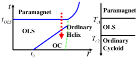
Figure 1: (Color online) (a) Phase diagram in Region I for the ordinary cycloid state. Solid (blue) lines represent second order phase transitions. Dotted (green) line indicates the first order transition to the helix state. The dotted (red) arrow represents one possible schematic locus of the experimental points obtained by varying $T$. $r_{0}\equiv\left(1+3D_{T}/D_{L}\right)/6$. (b) The sequence of phases with decreasing $T$ along the locus shown.

The OLS phase will, as we continue lowering $t$, eventually become unstable to a non-zero $m_{2}$; this is the OC state. By minimizing the energy (5) in the OLS phase, we find $q^{2}=q_{L,min}^{2}=-K_{0}/2D_{L}$ and $m_{1}^{2}={2}(t_{OLS}-t)/3u$. Inserting these into (5) we find that the coefficient of $m_{2}^{2}$ becomes negative below $t_{LOC}=t_{OLS}\left[3r-\left(1+3D_{T}/D_{L}\right)/2\right]$. This value $t_{LOC}$ of $t$ therefore defines the locus of a continuous OLS-OC phase transition, and is the non-horizontal straight (solid (blue)) line in the $r-t$ plane shown in Fig. 1a.

For $r>\sqrt{{\frac{D_{L}}{D_{T}}}}$, $\Gamma_{T}$ becomes non-zero first, which seems to imply that one enters the ordinary transverse spin density wave (OTS) phase ($m_{1}=m_{3}=0$, $m_{2}\neq 0$) first for large $r$. However, it is not true because the OTS phase always has higher energy than the ordinary helical (OH) phase. The energy for the ordinary helix state is

$$E/V=\Gamma_{T}(m_{1}^{2}+m_{2}^{2})+\Phi(m_{1}^{2},m_{2}^{2}).$$ (6)

The minimization of the energy over the direction of $\left(m_{1},m_{2}\right)$ vector yields $|m_{1}|=|m_{2}|=m_{H}/\sqrt{2}$, that is, a circular helix. Further minimization over $m_{H}$ and $q$ gives the energy $E_{OH}$ of the ordinary helix state $E_{OH}/V=-(t_{OH}-t)^{2}/4u{\ }$for $t<t_{OH}$, where $t_{OH}=r^{2}D_{L}t_{OLS}/D_{T}$. The energy for the OTS state is $E_{OTS}/V=-(t_{OH}-t)^{2}/6u$, which is obtained from equation (5) by setting $m_{1}=0$ and $q^{2}=q_{T,min}^{2}\equiv-\frac{K_{1}}{2D_{T}}$, and then minimizing over $m_{2}$. $E_{OTS}$ is clearly higher than $E_{OH}$. Hence, the helical state is always favored over the OTS state throughout Region I of the phase diagram. Note that $t_{OH}$ defines the boundary for the second order transition from the paramagnet to the OH state.

There is also a direct first order phase transition between the OH and the OLS states along the line where $E_{OH}=E_{OLS}$. Here $E_{OLS}/V=-(t_{OLS}-t)^{2}/6u$ is the energy for OLS state obtained from equation (5). This equality yields the first order phase boundary $t_{OLH}=(\sqrt{3/2}t_{OH}-t_{OLS})/(\sqrt{3/2}-1)$ between the OH and the OLS states (the dotted (green) line). The line for the OLS-OC transition always intersects the first order OLS-OH phase boundary before crossing the paramagnet-OLS boundary. This therefore always yields the topology shown in Fig. 1a.

A typical experimental locus through this phase diagram, namely one in which $t$ decreases as temperature $T$ does, with $r$ constant, is shown in Fig. 1a. The sequence of phases that results is illustrated in Fig. 1b. We see that the paramagnet to ordinary cycloid phase transition is always preempted by a paramagnet to OLS phase transition, and the cycloid state is always elliptical. Both of these predictions are borne out by recent experiments on TbMnO₃ Sneff ; Tokura3 . On the other hand, a direct transition to the circular helix state is predicted by our theory, and has indeed been observed experimentally Ishikawa ; Pfleiderer .

All of the above statements are based on mean field theory, that is theory without considering the fluctuations. Going beyond mean field theory, very general arguments due to Brazovskii Braz imply that, in rotation invariant models, any direct transition from a homogeneous state (paramagnet) to a translationally ordered one (OLS and OH) must be driven first order by fluctuations. Consideration of topological defects and orientational order Toner ; Toner2 ; Toner3 supports this conclusion, but raises the additional possibility that direct transition between the homogeneous and the translationally ordered phases could split into two, with an intermediate orientationally ordered phase, analogous to the 2D “hexatic” phase hexatic . In the present context, this implies that both the paramagnet to OLS and OH phase transitions are either driven first order by fluctuations, or split into two transitions with an intermediate orientationally ordered phase. Crystal symmetry breaking fields neglected in our model could invalidate this conclusion, if strong enough.

IV Conical Cycloid State

In Region II, we can show that conical cycloid (CC) state of the form $\mathbf{M}=\left(m_{1}\cos(qx),m_{2}\sin(qx),m_{3}\right)$ is the lowest energy state among all the possible states with arbitrary mutual angles between the uniform magnetization, $\mathbf{q}$, and the cycloid plane. The energy $E$ for this state takes the form

$$E/V = \left(t+K_{0}q^{2}+D_{L}q^{4}+2um_{3}^{2}\right)m_{1}^{2}/2$$

$$+\left(t+K_{1}q^{2}+D_{T}q^{4}+2um_{3}^{2}+K_{3}q^{2}m_{3}^{2}\right)m_{2}^{2}/2$$

$$+u\Phi(m_{1}^{2},m_{2}^{2})+tm_{3}^{2}+um_{3}^{4},$$

where we have again neglected the higher harmonics in Eq. (1). In this region, the h.h. terms do not vanish as the conical longitudinal spin density wave (CLS) ($m_{2}=0$, $m_{1,3}\neq 0$) or conical transverse spin density wave (CTS) ($m_{1}=0$, $m_{2,3}\neq 0$) to FM transition in Fig. 2 is approached. However, we have verified that amplitudes of the h.h. terms are only a very small fraction of the cycloidal components $m_{1}$ and $m_{2}$ (not of the uniform component $m_{3}$), therefore their neglect below (but close to) the lower cycloidal transition temperature of 26 K is justified. They have little or no quantitative effect on our phase diagram or the orders of the transition.

Since $t<0$, we can minimize Eq. (IV) over $m_{3}$ with $m_{1}=m_{2}=0$, and find a ferromagnetic (FM) state with $m_{3}=\sqrt{-t/2u}$. For large positive $K_{0}$ and $K_{1}$, this ferromagnetic state is clearly stable against the development of non-zero $m_{1}$ and $m_{2}$. It also clearly becomes unstable against the development of a non-zero $m_{1}$ if $K_{0}$ is lowered to negative values, because then the coefficient $(K_{0}q^{2}+D_{L}q^{4})$ of $m_{1}^{2}$ becomes negative for sufficiently small $q$. This instability (which is clearly into the CLS state) will occur at $K_{0}=0$, at a wavevector $q$ satisfying $q_{L,min}^{2}=-K_{0}/2D_{L}$. Note, however, that now, because $K_{0}$ is being varied through zero, this wavevector will now vanish as the transition is approached from below. The order parameter $m_{1}^{2}=K_{0}^{2}/2uD_{L}$ also vanishes as this transition is approached. Thus, this transition is, like the $\beta$ - incommensurate transition in quartz and berlinite Biham , simultaneously a nucleation transition ($q$ vanishes), and an instability transition (order parameter vanishes). Indeed, this transition and the FM$\rightarrow$ CTS transition, which is of the same type and will be discussed below, are, to our knowledge, the first examples of transitions that exhibit such a dual character in a model without terms linear in the gradient operator.

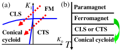
Figure 2: (Color online) (a) Phase diagram in Region II for the conical cycloid state. Solid (blue) lines are the boundaries between different phases. The dotted (red) arrows represent possible paths for transition to the CC state via continuous transitions. (b) The succession of the phases with decreasing $T$. The (green) arrow represents a direct first order transition between the FM and the CC state.

We can find the loci of instability between the CLS phase and the CC state by calculating the coefficient of $m_{2}^{2}$ in (IV) in the CLS phase, and finding where it becomes negative. The minimization of the energy (IV) over $q$, $m_{3}$ and $m_{1}$ yields $q^{2}=-K_{0}/2D_{L}$, $m_{3}^{2}=-\left(t+K_{0}^{2}/2D_{L}\right)/2u$ and $m_{1}^{2}=K_{0}^{2}/2uD_{L}$. Inserting these expressions into (IV) and taking the coefficient of $m_{2}^{2}$ to be zero, we find the CLS to CC phase boundary as:

$$K_{1}=\frac{K_{0}}{2}\left(\frac{D_{T}}{D_{L}}-1+\frac{K_{0}K_{3}}{2uD_{L}}\right)+\frac{tK_{3}}{2u}.$$ (8)

Similar analysis of the sequence of the phase transition, FM $\rightarrow$ CTS $\rightarrow$ CC, yields the schematic phase diagram on the $K_{0}-K_{1}$ plane given in Fig. 2a. The phase boundary between FM and CTS is given by $K_{1}=tK_{3}/2u$. The phase boundary between the CTS and the CC phase at small $K_{0}$ is $K_{1}=2K_{0}/\left(D_{L}/D_{T}-1\right)$, which is also shown in Fig. 2a.

Fig. 2 shows that it is not possible to go from the FM to the CC state via a continuous transition, except at a single special point. Generic paths like the diagonal dashed lines in Fig. 2a must go through either the CLS or the CTS state, so two transitions are required to reach the CC state, which, additionally, must be elliptical. Hence the only way there can be a direct transition from the FM state to the CC state is via a first order phase transition, which is not addressed by our theory. This prediction is borne out by experiments of CoCr₂O₄, where the direct FM to CC transition is indeed first order Tokura .

V Magnetic Reversal of the electric polarization:

The polarization $\bar{\mathbf{P}}=\chi\alpha m_{1}m_{2}\hat{y}$ in the CC state is in the $xy$ plane, normal to $\hat{e}_{3}$ and $\mathbf{q}$. It is independent of the uniform magnetization, $m_{3}$. Experimentally Tokura , the sample is cooled through $T_{c}$ in the presence of a small electric field, $\mathbf{E}=E_{0}\hat{y}$, and a small magnetic field, $\mathbf{H}=H_{0}\hat{z}$. The direction of the pitch vector, $\hat{x}$, or, equivalently, the axis of rotation, $\hat{z}$, are set by the direction of $\bar{\mathbf{P}}$ ($\mathbf{E}$), which determines the ‘helicity’ of the cycloid Tokura2 . It is found, at first, that $\bar{\mathbf{P}}$ is uniquely determined by $\mathbf{E}$ alone, independent of the initial direction of $\mathbf{H}$, as expected. However, once $\bar{\mathbf{P}}$ and $m_{3}$ have set in, changing $H_{0}$ to $-H_{0}$ not only reverses the direction of $m_{3}$, but also, quite unexpectedly, reverses the direction of $\bar{\mathbf{P}}$ as well. In the literature Mostovoy1 ; Tokura , this has lead to the definition of the ‘toroidal moment’, $\mathbf{T}=\mathbf{P}\times\mathbf{M}$, as the order parameter.

It is clear that the experimental system is in the conical cycloid state, where $m_{3},\mathbf{q}$ and $\bar{\mathbf{P}}$ are always in mutually orthogonal directions Tokura . Further, as expected for this state, the directions of $m_{3}$ and $\bar{\mathbf{P}}$ are uniquely determined by the small cooling fields, $\mathbf{H}$ and $\mathbf{E}$, respectively, which add terms to the Hamiltonian that split the degeneracy between the minima corresponding to the different directions. Now assume that the direction of $\mathbf{H}$ is reversed, $H_{0}\rightarrow-H_{0}$, reversing the direction of $m_{3}$ once it has well developed. There are two ways the uniform magnetization can reverse its direction. First, $m_{3}$ may continue to remain along the $z$-axis and its magnitude may pass through zero to become $-m_{3}$ for $\mathbf{H}=-H_{0}\hat{z}$. If this is the case, $\bar{\mathbf{P}}$ will remain fixed in the direction $\hat{y}$, since the mutual orthogonality of $m_{3},\mathbf{q}$ and $\bar{\mathbf{P}}$ can always be maintained and there is no direct coupling between $m_{3}$ and $\bar{\mathbf{P}}$. However, since $m_{3}$ is already well developed and large ($T_{m}=93$ K), due to the magnetic exchange energy cost it may be energetically more favorable to leave the magnitude of $m_{3}$ unchanged, and its direction may rotate in space to $-\hat{z}$. If this is the case, then $m_{3}$ must rotate staying on the $y-z$ plane, since that way it always remains perpendicular to $\mathbf{q}$, whose direction fluctuations cost the crystalline anisotropy energy. It is then clear, see Fig. 3, that the cycloid plane itself, which is always perpendicular to $m_{3}$ to maintain the lowest energy configuration, must rotate about $\hat{x}$ by a total angle $\pi$. It follows that $\bar{\mathbf{P}}$, always on the cycloid plane, reverses its direction to $-\hat{y}$. This way, even though there is no dynamical coupling between $m_{3}$ and $\bar{\mathbf{P}}$, the latter can also rotate by an angle $\pi$ as a result of the former reversing its direction in space. Based on this, we predict that, at some intermediate $\mathbf{H}\sim-H^{\prime}\hat{z}$, where $H^{\prime}<H_{0}$, $\bar{\mathbf{P}}$ points in the direction $-\hat{z}$, which can be experimentally tested.

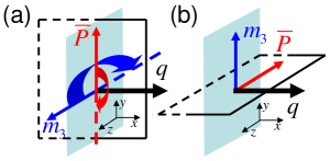
Figure 3: The reversal of the polarization ($\bar{\mathbf{P}}$) by the reversal of the magnetization ($m_{3}$). (a) If $m_{3}$ rotates to $-m_{3}$, remaining perpendicular to $\mathbf{q}$, the cycloidal ($xy$) plane must rotate accordingly to always remain transverse to $m_{3}$, which is the lowest energy configuration. Since $\bar{\mathbf{P}}$ is in the cycloidal plane, it will rotate by a total angle $\pi$. (b) An intermediate stage when $m_{3}$ has rotated by an angle $\frac{\pi}{2}$ and points in the $\hat{y}$ direction. At this stage, $\bar{\mathbf{P}}$ points in the $-\hat{z}$ direction.

VI Conclusions

To conclude, we’ve shown that the magnetic cycloidal orders, and the resulting multiferroicity, can naturally arise due to the magnetoelectric couplings even in rotationally invariant systems, or in cubic crystals. This explains such orders in CoCr₂O₄, which lack easy plane anisotropies, and are hence outside the realm of the previous theoretical studies on multiferroics. We also predict that a second order transition from the ferromagnet to the conical cycloid state can only occur through an intervening conical longitudinal or transverse spin density wave state with the ultimate cycloidal state being elliptical. A direct such transition, then, must be first order. An important feature of our Ginzburg-Landau theory is that we do not need to invoke an arbitrary (and ad hoc) ‘toroidal moment’ to explain the interplay between the magnetization and the polarization – the behavior which has been attributed to the toroidal moment arises naturally in our theory.

We thank D. Drew, D. Belitz, and R.Valdes Aguilar for useful discussions. This work is supported by NSF, NRI, LPS-NSA, and SWAN.

References

- (1) M. Fiebig, J. Phys. D: Appl. Phys. 38, R123 (2005).
- (2) S.-W. Cheong and M. Mostovoy, Nature Materials 6, 13 (2007).
- (3) Y. Tokura, Science 312, 1481 (2006).
- (4) R. Ramesh and N.A. Spaldin, Nature Materials 6, 21 (2007).
- (5) M. Mostovoy, Phys. Rev. Lett. 96, 067601 (2006).
- (6) G. Lawes, A. B. Harris, T. Kimura, N. Rogado, R. J. Cava, A. Aharony, O. Entin-Wohlman, T. Yildirim, M. Kenzelmann, C. Broholm, and A. P. Ramirez, Phys. Rev. Lett. 95, 087205 (2005).
- (7) T. Kimura, T. Goto, H. Shintani, K. Ishizaka, T. Arima and Y. Tokura, Nature 426, 55 (2003).
- (8) N. Hur, S. Park, P. A. Sharma, J. S. Ahn, S. Guha, S.W. Cheong, Nature 429, 392 (2004).
- (9) L.C. Chapon, G. R. Blake, M. J. Gutmann, S. Park, N. Hur, P. G. Radaelli, and S-W. Cheong, Phys. Rev. Lett. 93, 177402 (2004).
- (10) T. Goto, T. Kimura, G. Lawes, A. P. Ramirez, and Y. Tokura, Phys. Rev. Lett. 92, 257201 (2004).
- (11) M. Kenzelmann, A. B. Harris, S. Jonas, C. Broholm, J. Schefer, S. B. Kim, C. L. Zhang, S.-W. Cheong, O. P. Vajk, and J. W. Lynn, Phys. Rev. Lett. 95, 087206 (2005).
- (12) A. Pimenov, A. A. Mukhin, V. Yu. Ivanov, V. D. Travkin, A. M. Balbashov, A. Loidl, Nature Phys. 2, 97 (2006).
- (13) D. Senff, P. Link, K. Hradil, A. Hiess, L. P. Regnault, Y. Sidis, N. Aliouane, D. N. Argyriou, and M. Braden, Phys. Rev. Lett. 98, 137206 (2007).
- (14) Y. Yamasaki, H. Sagayama, T. Goto, M. Matsuura, K. Hirota, T. Arima, and Y. Tokura, Phys. Rev. Lett. 98, 147204 (2007).
- (15) Y. Yamasaki, S. Miyasaka, Y. Kaneko, J.-P. He, T. Arima, and Y. Tokura, Phys. Rev. Lett. 96, 207204 (2006).
- (16) H. Katsura, N. Nagaosa, and A. V. Balatsky, Phys. Rev. Lett. 95 057205 (2005).
- (17) I. A. Sergienko and E. Dagotto, Phys Rev. B 73, 094434 (2006).
- (18) H. Katsura, A. V. Balatsky, and N. Nagaosa, Phys. Rev. Lett. 98, 027203 (2007).
- (19) D. Belitz, T. R. Kirkpatrick, and A. Rosch, Phys. Rev. B 73, 054431 (2006).
- (20) B. R. Cooper, in Solid State Physics, edited by F. Seitz et al. (Academic Press, NY, 1968), Vol. 21, p.293.
- (21) Y. Ishikawa, K. Tajima, D. Bloch, M. Roth, Solid State Commun. 19, 525 (1976).
- (22) C. Pfleiderer, G. J. McMullan, S. R. Julian, and G. G. Lonzarich, Phys. Rev. B 55, 8330 (1997).
- (23) L. Lundgren, O. Beckman, V. Attia, S. P. Bhattacheriee, and M Richardson, Phys. Scr. 1, 69 (1970).
- (24) S. A. Brazovskii and S. G. Dmitriev, JETP 42, 497 (1976).
- (25) D. R. Nelson and J. Toner, Phys. Rev. B 24, 363 (1981).
- (26) J. Toner, Phys. Rev. A 27, 1157 (1983).
- (27) G. Grinstein, T. C. Lubensky, and J. Toner, Phys. Rev. B 33, 3306 (1986).
- (28) B. I. Halperin and D. R. Nelson, Phys. Rev. Lett. 41, 121 (1978).
- (29) O. Biham, D. Mukamel, J. Toner, and X. Zhu, Phys. Rev. Lett. 59, 2439 (1987).