AN ASYMMETRIC CONE MODEL FOR HALO CORONAL MASS EJECTIONS

Abstract

Due to projection effects, coronagraphic observations cannot uniquely determine parameters relevant to the geoeffectiveness of CMEs, such as the true propagation speed, width, or source location. The Cone Model for Coronal Mass Ejections (CMEs) has been studied in this respect and it could be used to obtain these parameters. There are evidences that some CMEs initiate from a flux-rope topology. It seems that these CMEs should be elongated along the flux-rope axis and the cross section of the cone base should be rather elliptical than circular. In the present paper we applied an asymmetric cone model to get the real space parameters of frontsided halo CMEs (HCMEs) recorded by SOHO/LASCO coronagraphs in 2002. The cone model parameters are generated through a fitting procedure to the projected speeds measured at different position angles on the plane of the sky. We consider models with the apex of the cone located at the center and surface of the Sun. The results are compared to the standard symmetric cone model.

1 Introduction

A halo coronal mass ejection (HCME) was first recorded by Howard in 1982 (Howard et al., 1982). Since then, HCME are routinely recorded in white light by coronagraphs placed in space. In coronagraphic observations, HCMEs appear as an enhancement surrounding the entire occulting disk. HCMEs originating close to the disk center are often responsible for the severest geomagnetic storms (Gosling, 1993; Kahler, 1992; Webb et al., 2000). For space weather forecast it is very important to determine the kinetic and geometric parameters describing HCMEs. Unfortunately coronagraphic observations are subjected to projection effects. Viewing in the plane of the sky does not allow to determine the true 3-D space velocity, width and source location of a given CME. It is widely accepted that the geometrical structure of CMEs may be described by the cone model (e.g., Howard et al., 1982; Fisher and Munro, 1984; St.Cyr et al., 2000; Webb et al, 2000; Zhao et al., 2002; Michalek et al., 2003; Xie et al., 2004; Xue et al., 2005). Assuming that the shape of HCMEs is a cone and they propagate with constant angular widths and speeds, at least in their early phase of propagation, a technique was developed (Michalek et al., 2003) which can determine the following parameters: the linear distance $r$ of the source location measured from the solar disk center, the angular distance $\gamma$ of the source location measured from the plane of the sky, the angular width $\alpha$ (cone angle =$0.5\alpha$) and the 3-D space velocity $V_{S}$ of a given HCME. This technique required measurements of the sky-plane speed and the moment of the first appearance of the halo CME above opposite limbs. If we determine spatial parameters using only two measurements, large random errors would occur. What is more, this technique was limited to asymmetric events not originating from close to the center of the Sun. A similar cone model was used recently by Xie et al. (2004) to determine the angular width and orientation of HCMEs. To improve accuracy, in the present attempt the space parameters of HCMEs are determined by fitting the cone model to projected speeds ($V_{P}$) obtained from height-time plots at different position angles. Although many thousands of CMEs were recorded by LASCO coronagraphs the 3D structure of CMEs is still open question. Many authors believe that CMEs originate from a flux-rope geometry, (e.g., Chen et al., 1997; Dere et al., 1999; Chen et al., 2000; Plunket et al., 2000; Forbes 2000; Krall et al., 2001; Chen and Krall 2003). If CMEs have a flux-rope geometry, they should be elongated along the flux-rope axis and the cross section of the cone base should be rather elliptical than circular. In the present approach we consider the asymmetric cone model where an eccentricity and orientation of the cone base are new free parameters. We try to identify where to locate the apex of the cone, either at the center of the Sun (Zhao et al., 2002; Xie et al., 2004) or on the solar surface (Michalek et al., 2003). It is important to note that the real elliptical cone model was first developed by Cremades and Bothmer (2004). The model was introduced based on observations of cylindrical shaped CMEs (Cremades and Bothmer, 2004, 2005). They applied it to 32 halo CMEs. In their approach, the best parameter values describing the ellipse are determined from a LASCO image sequence that showed a sharp leading edge. In our method we derive the best-fit parameter values for halo CMEs by working in the velocity space. The paper is organized as follows: in Section 2 the asymmetric cone model is presented, numerical simulations and fitting procedure are explained in Section 3 and in Section 4 the results are described. Final conclusions are given in Section 5.

2 The Asymmetric Cone Model of CMEs

In the projection on the sky, most of the CMEs (especially limb events) observed by the LASCO coronagraphs look like cone-shaped blobs. The observed angular widths, for many limb events, remain nearly constant as a function of height (see, e.g., Webb et al., 1997). Most of them propagate with a constant radial frontal speed but many slow CMEs gradually accelerate whereas many fast CMEs decelerate (St. Cyr et al., 2000; Sheeley et al., 1999; Gopalswamy et al., 2001; Yashiro et al., 2004). Assuming that CMEs propagate with a constant velocity and angular width, many authors reproduced them (Howard et al., 1982; Fisher and Munro 1984; Zhao et al., 2002; Michalek et al., 2003, Xie et al., 2004) using the cone model defined by four parameters: velocity, angular width, and orientation of the central axis of the CME (longitude and latitude). As was mentioned above, many CMEs originate from the flux-rope geometry and their cone shape may not be perfectly symmetrical. This was also demonstrated recently by Moran and Davila (2004), Cramades and Bothmer (2004) and Jackson et al. (2004). This encouraged us to introduce the asymmetric cone model. In the asymmetric cone model we assume that (1) the shape of CMEs is a cone but its cross section is not a circle but ellipse and (2) the velocity and shape of CMEs (angular widths measured along the major and minor axes of the ellipse) remain constant during their early phase of propagation. The eccentricity and orientation of the elliptic cone cross section appear as the additional two parameters of the model. We also consider two possibilities, namely the apex of the cone is located at the center of the Sun and on the surface of the Sun.

To obtain relationships between the measured velocities and the cone model parameters we had to apply the transformation between two coordinate systems: First, a heliocentric coordinate system (HCS) ($x_{h},y_{h},z_{h}$), where $x_{h}$ points to Earth, $z_{h}$ points north and $y_{h}-z_{h}$ defines the sky plane. Second, an apex-centered cone coordinate system (CCS) ($x_{c},y_{c},z_{c}$) whose origin is at the apex of the cone, $z_{c}$ is the cone axis, and $x_{c}-y_{c}$ defines the plane parallel to the base of the cone. The orientation of the cone is determined by heliographic longitude ($\varphi$) and latitude ($\lambda$) measured from the central meridian and the solar equator, respectively. If the apex of the cone is at the center of the Sun, the transformation from the HCS to the CCS can be carried out by double rotations. The first rotation is about the $x_{h}$ axis through the angle $\varphi$. The second rotation is about the $y_{h}$ axis through the angle $90^{o}-\lambda=\vartheta$. This transformation in matrix notation can be written as:

$$\left(\matrix{x_{h}\cr y_{h}\cr z_{h}}\right)=\left(\matrix{&\cos\vartheta\cos\varphi&-\sin\varphi&\cos\varphi\sin\varphi\cr&\cos\vartheta\sin\vartheta&\cos\varphi&\sin\varphi\sin\vartheta\cr&-\sin\varphi&0&\cos\vartheta}\right)\left(\matrix{x_{c}\cr y_{c}\cr z_{c}}\right)$$

or

$$\left(\matrix{x_{c}\cr y_{c}\cr z_{c}}\right)=\left(\matrix{&\cos\vartheta\cos\varphi&\cos\vartheta\sin\varphi&-\sin\vartheta\cr&-\sin\varphi&\cos\varphi&0\cr&\cos\varphi\sin\vartheta&\sin\varphi\sin\vartheta&\cos\vartheta}\right)\left(\matrix{x_{h}\cr y_{h}\cr z_{h}}\right).$$

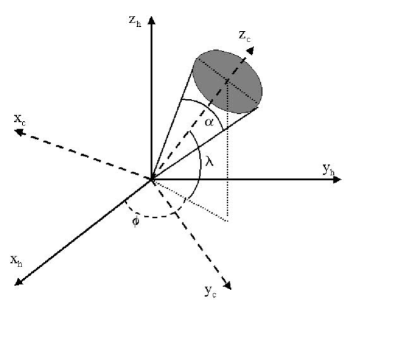
Figure 1: The cone model topology and relationship between the heliocentric coordinate system and the cone coordinate system when the cone apex is placed at the center of the Sun.

In Figure 1, the cone model topology and the relationship between the HCS and the CCS is shown. If the apex of the cone is on the surface of the Sun, these relationships are slightly modified. The transformation from the HCS to the CCS can be carried out by double rotations and additional shifting of the origin to the surface of the Sun. Then we obtain:

$$\left(\matrix{x_{h}\cr y_{h}\cr z_{h}}\right)=\left(\matrix{&\cos\vartheta\cos\varphi&-\sin\varphi&\cos\varphi\sin\varphi\cr&\cos\vartheta\sin\vartheta&\cos\varphi&\sin\varphi\sin\vartheta\cr&-\sin\varphi&0&\cos\vartheta}\right)\left(\matrix{x_{c}\cr y_{c}\cr z_{c}}\right)+\\ \left(\matrix{R_{S}\sin\vartheta\cos\varphi\cr R_{S}\sin\vartheta\sin\varphi\cr R_{S}\cos\vartheta}\right)$$

or

$$\left(\matrix{x_{c}\cr y_{c}\cr z_{c}}\right)=\left(\matrix{&\cos\vartheta\cos\varphi&\cos\vartheta\sin\varphi&-\sin\vartheta\cr&-\sin\varphi&\cos\varphi&0\cr&\cos\varphi\sin\vartheta&\sin\varphi\sin\vartheta&\cos\vartheta}\right)\left(\matrix{x_{h}\cr y_{h}\cr z_{h}}\right)-\left(\matrix{R_{S}\sin\vartheta\cos\varphi\cr R_{S}\sin\vartheta\sin\varphi\cr R_{S}\cos\vartheta}\right)$$

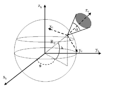
Figure 2: The cone model topology and relationship between the heliocentric coordinate system and the cone coordinate system when the cone apex is placed on the surface of the Sun.

where $R_{S}$ is the solar radius. The topology of the cone model in this case is demonstrated in Figure 2. Using these transformations, we can find the angle ($\sigma$) between a generatrix of the cone and the plane of the sky (Xue et al., 2005):

$$\sin\sigma={\cos{\alpha\over 2}\cos\varphi\sin\vartheta-A\sqrt{\cos^{2}\varphi\sin^{2}\varphi+A^{2}-\cos^{2}{\alpha\over 2}}\over\cos^{2}\varphi\sin^{2}\varphi-A^{2}}$$

where

$$A=\cos\psi\sin\varphi\sin\vartheta+\sin\psi\cos\vartheta$$

and $\psi$ is the azimuthal angle of a given cone generatrix in the plane of sky. The basic equation for our consideration is the relationship between the projected velocities ($V_{P}$, derived from LASCO height-time plots) and the 3-D space velocities ($V_{S}$, a parameter in the cone model):

$$V_{P}=V_{S}\cos\sigma.$$

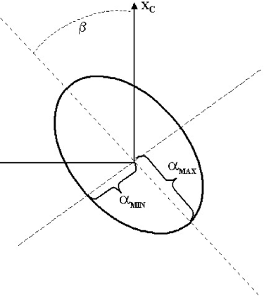
Figure 3: The cone base topology in the cone coordinate system.

We have to note that we presented the relationships of Equations (6) and (7) only for the model in which the cone apex is at the center of the Sun. For another possibility (when the cone apex is placed on the surface of the Sun), equations become more complicated. It is evident that $V_{P}$ depends on $V_{S}$, the location of the origin (cone apex) on the Sun (longitude-$\varphi$, latitude-$\lambda$), and the width ($\alpha$) of the cone. The above formulae are also applicable to the symmetric cone model. We improved these formulae by considering an asymmetric cone namely the base of the cone has an elliptical shape. In Figure 3 the topology of the cone base in the cone coordinate system is presented. This modification introduces the eccentricity and orientation of the ellipse as new parameters. In this paper the eccentricity is defined as:

$$e=\sqrt{\alpha_{\textrm{\tiny{MAX}}}^{2}-\alpha_{\textrm{\tiny{MIN}}}^{2}\over\alpha_{\textrm{\tiny{MAX}}}^{2}}$$

where $\alpha_{\textrm{\tiny{MAX}}}$ and $\alpha_{\textrm{\tiny{MIN}}}$ are the angular widths of the cone cross section along the major and minor axes of the ellipse, respectively. This parameter should depend on the separation of the foot points and width of the flux rope. The orientation of the ellipse (the position angle of the major axis) should depend on the orientation of the foot points of the flux rope. The flux-rope could be oriented in a random way on the solar disk, so we need to consider the next free parameter of the model: the orientation of the ellipse ($\beta$) which is defined as the azimuthal angle of the main axis of the ellipse measured in the plane $x_{c}-y_{c}$. To use the formula (7) to determine the space parameters of CMEs we need to express $\alpha$ as a function of position angle ($\psi$) measured in the plane of the sky. First, we can define $\alpha$ as a function of angle $\gamma$. From the definition of the ellipse and Figure 3 we can write:

$$\alpha_{1/2}=\sqrt{({\alpha_{\textrm{\tiny{MAX}}}\over 2})^{2}\cos(\delta-\beta)+({\alpha_{\textrm{\tiny{MIN}}}\over 2})^{2}\sin(\delta-\beta)}.$$

This equation shows the dependence of $\alpha$ on the position angle ($\gamma$), measured in the cone coordinate system. The next step is to transform the angle $\gamma$ to the position angle measured in the plane of the sky. From Equation (1), neglecting dependence on $Z_{c}$, we can get:

$$\cot(\psi)={Y_{h}\over Z_{h}}=-\cot(\theta)\sin(\phi)-{Y_{c}\over X_{c}}{\cos(\phi)\over\sin(\theta)}.$$

Noting that ${Y_{c}\over X_{c}}=\cot(90^{o}-\delta)=\tan(\delta)$ we can finally write:

$$\tan(\delta)=[-\cot(\theta)\sin(\phi)-\cot(\psi)]{\sin(\theta)\over\cos(\phi)}.$$

Now we have all necessary equations to consider the asymmetric cone model. Using Equations (9) and (11) we can define $\alpha$ as a function of the position angle ($\psi$). It is important to note that, to be strictly consistent with the assumption of constant velocities of CMEs, the base of the cone (an ellipse) must be on a sphere, not on a plane. This needs to introduce a new parameter, a radius of the sphere, which changes together with an expansion of CMEs and is very difficult to estimate. Therefore, in our study, we assume that the base of the cone is a planar ellipse expanding radially with the same speed everywhere on the ellipse. This is a simplification in our model which we believe would not introduce severe inconsistency in the model.

Summarizing, we have seven parameters describing the asymmetric cone model: the expansion velocity in 3-D space ($V_{S}$), the angular width of the cone ($\alpha_{\textrm{\tiny{MAX}}}$, measured along the major axis), the longitude of the cone axis ($\varphi$), the latitude of the cone axis ($\lambda$), the eccentricity of the cone cross section ($e$), the orientation of the main axis of the cone cross section ($\beta$) and finally the localization of the cone apex (on the surface ($S$) or at the center of the Sun ($C$)). Using these parameters we can determine two more parameters which are typically used to characterize the cone model: the angle between the central axis of the cone and the plane of the sky ($\gamma$) and the position angle of the farthest (fastest-movinng) structure of CME ($PAM$). We obtain them by the following relationships:

$$\sin\gamma=\sin\vartheta\cos\varphi$$

and

$$\tan PAM={\sin\vartheta\cos\varphi\over\cos\vartheta}.$$

$PAM$ is measured from solar north in degrees.

3 Determination of parameters describing HCMEs

We applied the asymmetric cone model to obtain the parameters of frontsided HCMEs recorded by SOHO/LASCO coronagraphs in 2002. We considered HCMEs originating close to the disk center ($|\varphi|<30^{o}$) only. These events are clear HCMEs (in contrast to limb events appearing as halos due to deflections of pre-existings coronal structures) and they are sufficiently bright to obtain height-time plots around the entire occulting disk. Two main reasons for looking at these events more closely are: (1) they are responsible for severe geomagnetic storms and (2) not all such symmetric events were considered by Michalek et al. (2003). A two-step procedure was carried out to obtain the parameters characterizing HCMEs. First, using the height-time plots the projected speeds at different position angles were determined. We made measurements, for the considered events, every $15^{o}$ around the entire occulting disk. This allowed us to obtain $24$ points for each event which are required for the fitting procedure. Second, using numerical simulation through minimizing the root mean square error the cone model parameters were obtained. The simulation procedure was also performed in two steps. First, we executed simulations without any constraints on the cone parameters. These simulations performed with small accuracy produced only approximate values for the cone parameters. Next, more precise simulations (with constraints on the cone parameters) with better accuracy were made to obtain the final best-fit cone model parameters. To compare the asymmetric (new) and symmetric (standard) cone model we performed both types of simulations. The results of our studies are presented in the next section.

4 Results

During 2002 we selected 15 frontsided HCMEs originating close to the disk center ($|\varphi|\leq 30^{o}$). For all of them, the cone parameters using the asymmetric (ACM) and symmetric cone models (SCM) were determined. The results for the ACM and SCM are presented in Tables I and II, respectively. The first four columns are from the SOHO/LASCO catalog and give the date, time of the first appearance in the coronagraph field of view, projected speed and position angle of the farthest (fastest-moving) part of the HCME. In column (5) the source locations of the associated H-alpha flares are presented. Parameters $\alpha$, source locations and $V_{S}$ estimated from the cone model are shown in columns (6), (7), and (8), respectively. In column (9) the r.m.s errors (in km s^-1) for the best fits are given. The parameters $\gamma$ and $PAM$ are shown in columns (10) and (11), respectively. These data are presented in both tables. In Table I, we have three additional columns displaying the new parameters used only for the asymmetric cone model. In columns (12) and (13), the eccentricity ($e$) and orientation of the cone base ($\beta$) are presented. In the last column (14) the location of the cone apex is described ($S$: surface of the Sun, $C$: center of the Sun). Figures 4-17 are polar plots showing the fitted projected speeds (solid lines) and measured projected speeds (cross symbols) in the velocity space. Left and right panels are for the ACM and the SCM models, respectively. From the polar plots and the r.m.s errors presented in the tables it is evident that the ACM fits much better the measured projected speeds in comparison with the SCM. For all considered events the r.m.s errors are much smaller for the ACM than for the SCM. The average r.m.s errors for all events are equal to 60 km s^-1 and 84 km s^-1 for the ACM and SCM, respectively. If CMEs could be considered as the symmetric cones then their projected speed should also follow the elliptic shapes in the plane of the sky. Checking Figures 4-17, we see that the measured projected speeds for all considered events show more complicated structures which can not be fitted by the SCM. Only the ACM can adjust shapes indicated by the measured projected speed with good accuracy. From the inspection of the tables, we see that the cone parameters obtained from both models are slightly different. On average, the space velocities are about 50 km s^-1 higher and the cone widths are about $4^{o}$ lower for the SCM in comparison with the ACM. If we consider the ACM only, it is evident that more events (11 out of 15) have better fits when the cone apex is placed in the center of the Sun. This means that CMEs are likely to originate from the finite area but not from the point source. It is important to note, that all events with velocities above 1200 km s^-1 have better fits when the cone apex is placed at the center of the Sun. It seems obvious that powerful events need more energy input. The eccentricity ($e$) and orientation of the cone base ($\beta$), for the considered events, vary in a random way between $0.8-0.4$ and $0^{o}-180^{o}$, respectively. Using our model (working in the velocity space) we can also reconstruct the space shapes (in the plane of sky) of CMEs. Figure 17 shows an example of LASCO CME (halo CME from 2002/03/15) with dark dots representing the projected radial distances derived from the ACM. To obtain these dots we assumed that the onset of this CME was at 22:09UT (X-ray flare onset) on 15 March 2002. We can see that the model reproduces the space shape of the CME very well.

5 Summary

In this paper we have presented the new asymmetric cone model to determine the geometrical parameters characterizing HCMEs. We applied this model to all frontsided HCMEs originating close to the disk center and listed in the SOHO/LASCO catalog in 2002. We estimated, with very good accuracy (the average r.m.s error is equal to 60 km s^-1), the cone parameters for $15$ events. It was shown (from the polar plots and the r.m.s errors) that the ACM can reproduce, around the entire occulting disk, the measured projected speed much better than the SCM. We have to note that sometimes the individual projected speeds may significantly differ from the fitting model even for the ACM. In these cases errors are probably caused by inaccurate measurements. Unfortunately, most HCMEs are not sufficiently bright around the entire occulting disk to generate the height-time plots with the same good accuracy for all considered position angles. The biggest errors may arise when the faintest part of a given event is considered or when measurements are disturbed by another event appearing in the LASCO field of view. We also confirmed that most of the events have better fits when the cone apex is located at the center of the Sun. We used this model for the frontsided full HCMEs originating close to the disk center but it can also be applied to limb and even partial HCMEs. When considering limb or partial HCMEs the accuracy will be slightly worse. The determined parameters for HCMEs are similar to that derived by the other cone models, but for some events differences could amount to even 20%. We have to remember that this approach has two shortcomings: (1) CMEs may be accelerating, moving with constant speed or decelerating at the beginning phase of propagation. This means that the constant velocity assumption may be invalid.(2) CMEs may expand in addition to radial motion. Then the measured sky-plane speed is a sum of the expansion speed and the projected radial speed. This would also imply that CMEs may not be a rigid cone as we had assumed. Unfortunately, having observation from only one spacecraft there is no possibility to overcome these assumptions. There are two attempts to get the real space parameters of CMEs. Some scientist (e.g. Xie et al., 2004) try to get the real parameters of CMEs by considering the elliptical shapes of observed CMEs. In our approach we consider velocities of CMEs as a function of the position angle. We take into account the projected velocities (many points) from an entire halo CME, not only from a few chosen points. We do not introduce any assumption about the apparent (geometrical) shapes of CMEs. Therefore, we expect that our determination of parameters may have better accuracy. The determined real velocities of halo CMEs could be potentially useful for space weather forecast. But we have to note that although it is true that faster interplanetary CMEs are more geoeffective, the strength and topology of magnetic field is still crucial to define geoeffectiveness of CMEs (e.g., Bothmer, 2003).

Figure 4: The polar plots for the HCME on 2002/03/15 showing the fitted projected speeds (solid lines) and measured projected speeds (cross symbols) in the velocity space. For comparison the best fits for the asymmetric cone model (left panel) and the symmetric cone model (right panel) are presented.

Figure 5: The polar plots for the HCME on 2002/03/18. The format is the same as in Figure 4.

Figure 6: The polar plots for the HCME on 2002/04/01. The format is the same as in Figure 4.

Figure 7: The polar plots for the HCME on 2002/04/15. The format is the same as in Figure 4.

Figure 8: The polar plots for the HCME on 2002/05/07. The format is the same as in Figure 4.

Figure 9: The polar plots for the HCME on 2002/05/08. The format is the same as in Figure 4.

Figure 10: The polar plots for the HCME on 2002/05/16. The format is the same as in Figure 4.

Figure 11: The polar plots for the HCME on 2002/07/15. The format is the same as in Figure 4.

Figure 12: The polar plots for the HCME on 2002/07/16. The format is the same as in Figure 4.

Figure 13: The polar plots for the HCME on 2002/07/18. The format is the same as in Figure 4.

Figure 14: The polar plots for the HCME on 2002/07/26. The format is the same as in Figure 4.

Figure 15: The polar plots for the HCME on 2002/08/16. The format is the same as in Figure 4.

Figure 16: The polar plots for the HCME on 2002/09/05. The format is the same as in Figure 4.

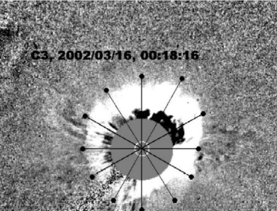
Figure 17: The halo CME recorded by LASCO/C3 coronagraph on 16 March 2002 at 00:18 UT (In LASCO catalog it is halo CME from 2002/03/15). Dark dots represent radial distances derived for this event from ACM.

Table I
List of halo CMEs with parameters derived from the ACM.

Date	Time	Speed	PA	Flare	$\alpha_{\tiny MAX}$	Location	V	Error	$\gamma$	PAM	e	$\beta$	Cone Apex
		km s-1	Deg		Deg		km s-1	km s-1	Deg	Deg		Deg
2002/03/15	23:06:06	957	309	S08W03	95	N07W01	1178	47	81	347	0.6	75	S
2002/03/18	02:54:06	989	311	S04W24	114	N11W22	947	42	64	296	0.6	90	C
2002/04/01	13:25:05	474	350	N11E21	167	N35E30	747	46	46	35	0.6	45	C
2002/04/15	03:50:05	720	198	S18W01	168	N14W21	715	27	66	304	0.4	60	C
2002/05/07	04:06:05	720	112	S22E14	44	S03E08	1258	39	81	110	0.4	90	C
2002/05/08	13:50:05	614	229	S12W07	77	S08W08	657	55	78	224	0.7	120	S
2002/05/16	00:50:05	600	158	S22E14	60	S12E06	915	38	77	153	0.6	75	C
2002/07/15	20:30:05	1151	35	N19W01	67	N18E10	1249	28	69	28	0.6	135	C
2002/07/16	16:02:58	1636	325	N23W07	70	N05W01	2268	150	85	348	0.8	45	C
2002/07/18	08:06:08	1099	354	N19W30	104	N20W13	1110	66	66	328	0.7	75	S
2002/07/26	22:06:10	818	172	S19E26	80	S21E13	846	36	65	149	0.6	150	S
2002/08/16	12:30:05	1585	121	S14E20	72	S14E06	1895	68	74	157	0.4	150	C
2002/09/05	16:54:06	1748	114	N09E28	41	S08E12	2758	52	75	123	0.4	15	C
2002/11/09	13:31:45	1838	233	S12W29	52	S08W09	2658	100	78	228	0.6	105	C
2002/12/19	22:06:05	1092	300	N15W09	67	N06W01	2504	110	84	352	0.7	45	C

Table II
List of halo CMEs with parameters derived from the SCM.

Date	Time	Speed	PA	Flare	$\alpha$	Location	V	Error	$\gamma$	PAM
		km s-1	Deg		Deg		km s-1	km s-1	Deg	Deg
2002/03/15	23:06:06	957	309	S08W03	72	N05W01	1375	62	85	348
2002/03/18	02:54:06	989	311	S04W24	121	N09W23	969	57	65	292
2002/04/01	13:25:05	474	350	N11E21	156	N31E32	738	66	46	41
2002/04/15	03:50:05	720	198	S18W01	169	N10W21	692	30	67	296
2002/05/07	04:06:05	720	112	S22E14	48	S04E09	1110	38	80	113
2002/05/08	13:50:05	614	229	S12W07	58	S06W06	818	69	81	225
2002/05/16	00:50:05	600	158	S22E14	54	S12E06	934	49	77	153
2002/07/15	20:30:05	1151	35	N19W01	54	N16E08	1520	55	74	29
2002/07/16	16:02:58	1636	325	N23W07	58	N04W01	2467	235	86	346
2002/07/18	08:06:08	1099	354	N19W30	84	N18W12	1128	101	66	326
2002/07/26	22:06:10	818	172	S19E26	96	S25E16	804	41	60	149
2002/08/16	12:30:05	1585	121	S14E20	103	S15E06	1852	78	73	158
2002/09/05	16:54:06	1748	114	N09E28	47	S08E12	2770	56	75	123
2002/11/09	13:31:45	1838	233	S12W29	46	S08W09	2770	137	78	228
2002/12/19	22:06:05	1092	300	N15W09	62	N06W01	2506	179	84	353