Bayesian Treed Gaussian Process Models with an Application to Computer Modeling

Abstract

Motivated by a computer experiment for the design of a rocket booster, this paper explores nonstationary modeling methodologies that couple stationary Gaussian processes with treed partitioning. Partitioning is a simple but effective method for dealing with nonstationarity. The methodological developments and statistical computing details which make this approach efficient are described in detail. In addition to providing an analysis of the rocket booster simulator, our approach is demonstrated to be effective in other arenas.

Key words: computer simulator, recursive partitioning, nonstationary spatial model, nonparametric regression, heteroscedasticity

1 Introduction

Much of modern engineering design is now done through computer modeling, which is both faster and more cost-effective than building small-scale models, particularly in the earlier stages of design when more scope for changes is desired. As design proceeds, increasingly sophisticated simulators may be created. Our work here was motivated by a simulator of a proposed rocket booster. NASA relies heavily on simulators for design, as wind tunnel experiments are quite expensive and still not fully realistic of the range of flight experiences. In particular, one of the highly critical points in time for a rocket booster is the moment that it re-enters the atmosphere. Such conditions are difficult to recreate in a wind tunnel, and it is obviously impossible to run a standard physical experiment. Thus to learn about the behavior of the proposed rocket booster, NASA uses computer simulation.

Simulators can involve large amounts of physical modeling, requiring the numerical solution of complex systems of differential equations. The NASA simulator was no exception, typically requiring between five and twenty hours for a single run. Thus, NASA was interested in creating a statistical model of the simulator itself, an emulator or surrogate model, in the terminology of computer modeling. The standard approach in the literature for emulation is to model the simulator output with a stationary smooth Gaussian process (GP) (Sacks et al.,, 1989; Kennedy and O’Hagan,, 2001; Santner et al.,, 2003). However, this approach proved to be inadequate for the NASA data. In particular, we were faced with problems of nonstationarity, heteroscedasticity, and the size of the dataset. Thus we introduce here an expansion of GPs, based on the idea of Bayesian partition models (Chipman et al.,, 2002; Denison et al.,, 2002), which is able to address these issues.

GPs are conceptually straightforward, can easily accommodate prior knowledge in the form of covariance functions, and can return estimates of predictive confidence, which were desired by NASA. However, we highlight three disadvantages of the standard form of a GP which we had to confront on this dataset, and expect to encounter on a wide range of other applications. First, inference on the GP scales poorly with the number of data points, $N$, typically requiring computing time in $O(N^{3})$ for calculating inverses of $N\times N$ covariance matrices. Second, GP models are usually stationary in that the same covariance structure is used throughout the entire input space, which may be too strong of a modeling assumption. Third, the estimated predictive error (as opposed to the predictive mean value) of a stationary model does not directly depend on the locally observed response values. Rather, the predictive error at a point depends only on the locations of the nearby observations and on a global measure of error that uses all of the discrepancies between observations and predictions without regard for their distance from the point of interest (because of the stationarity assumption). (Section 4.3 provides more details, in particular note that Eq. (12) does not depend on ${\bf z}$.) In many real-world spatial and stochastic problems, such a uniform modeling of uncertainty will not be desirable. Instead, some regions of the space will tend to exhibit larger variability than others. On the other hand, fully nonstationary Bayesian GP models (e.g., Higdon et al.,, 1999; Schmidt and O’Hagan,, 2003) can be difficult to fit, and are not computationally tractable for more than a relatively small number of datapoints. Further discussion of nonstationary models is deferred until the end of Section 3.2.

All of these shortcomings can be addressed by partitioning the input space into regions, and fitting separate stationary GP models within each region (e.g., Kim et al.,, 2005). Partitioning provides a relatively straightforward mechanism for creating a nonstationary model, and can ameliorate some of the computational demands by fitting models to less data. A Bayesian model averaging approach allows for the explicit estimation of predictive uncertainty, which can now vary beyond the constraints of a stationary model. Finally, an R package with implementations of all of the models discussed in this paper is available at
http://www.cran.r-project.org/web/packages/tgp/index.html. We note that by partitioning, we do not have any theoretical guarantee of continuity in the fitted function. However, as we demonstrate in several examples, Bayesian model averaging yields mean fitted functions that are typically quite smooth in practice, giving fits that are indistinguishable from continuous functions except when the data call for the contrary. Indeed the ability to accurately model possible discontinuities is a side benefit of this approach.

The rest of the paper is organized as follows. Section 2 describes the motivating data in further detail. Section 3 provides some background material. Section 4 combines stationary GPs and treed partitioning to create treed GPs, implementing a tractable nonstationary model for nonparametric regression. In Section 5 we return to the analysis of the rocket booster data, and in Section 6 we conclude with some discussion.

2 The Langley Glide-Back Booster Simulation

The Langley Glide-Back Booster (LGBB) is a proposed rocket booster under design at NASA. Standard rocket boosters are created to be reusable, assisting in the launch process and then parachuting back to the Earth after their fuel has been exhausted. Their return path is planned so that they fall into the ocean, where they can be recovered and reused. The LGBB represents a new direction in booster design, as it would have wings and a tail, looking somewhat similar to the space shuttle. The idea is that it would gracefully glide back down, rather than plummeting into the ocean.

The development of the booster is being done primarily through the use of computer simulators. The particular model (Rogers et al.,, 2003) with which we were involved is based on computational fluid dynamics simulators that numerically solve the relevant inviscid Euler equations over a mesh of 1.4 million cells. Each run of the Euler solver for a given set of parameters can take 5-20 hours on the NASA computers. The simulator is theoretically deterministic, but the solver is typically started with random initial conditions and does not always numerically converge. There is an automated check for convergence which is mostly accurate, but some runs are marked as accepted despite their false convergence, or they converge to a clearly inferior local mode. For those runs that fail the automated convergence check, the solver is restarted at a different set of randomly chosen initial conditions. Our NASA collaborators have commented that input configurations arbitrarily close to one another can fail to achieve the same estimated convergence, even after satisfying the same stopping criterion. Thus neither simple interpolation of the data nor a Gaussian process model without an error term will be adequate, as smoothing will be necessary to reduce the impact of the inaccurate runs.

The simulator models the forces felt by the vehicle at the moment it is re-entering the atmosphere. As a free body in space, there are six degrees of freedom, so the six relevant forces are lift, drag, pitch, side-force, yaw, and roll. For this project, the interest focused just on the lift force, as that is the most important one for keeping a vehicle aloft. The inputs to the simulator are the speed of the vehicle at re-entry (measured by Mach number), the angle of attack (the alpha angle), and the sideslip angle (the beta angle). Thus the primary goal is to model the lift force as a function of speed, alpha, and beta. The sideslip angle is quantized in the experiments, so it is run only at six particular levels. Speed ranges from Mach 0 to 6, and the angle of attack, alpha, varies from negative five to thirty degrees. The simulator was run at 3041 locations, over a combination of three hand-designed grids. The first grid was relatively coarse and was equally spaced over the whole region of interest. Two successively finer grids on smaller regions primarily around Mach one were further run, as the initial run showed that the most interesting part of the input space was generally around the sound barrier. This makes sense because the physics in the simulator comes from two completely different regimes, a subsonic regime for speeds less than Mach one, and a supersonic regime for speeds greater than Mach one. What happens close to and along the boundary is the most difficult part of the simulation.

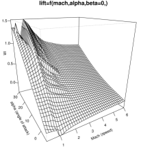
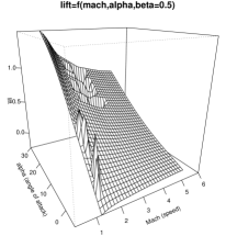
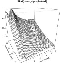
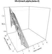
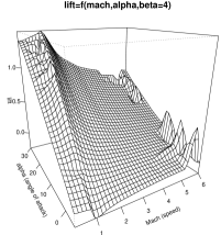
Figure 1: Interpolation of lift by speed and angle of attack for all sideslip levels. Note that for levels 0.5 and 3 (center), Mach ranges only in $(1,5)$ and $(1.2,2.2)$.

The upper-left plot in Figure 1 shows an interpolation of the simulator output for the lift surface as a function of speed and angle of attack, when the sideslip angle is zero. The primary feature of this plot is the large ridge which appears at Mach one and larger angles of attack. The transition from subsonic to supersonic is a sharp one, and it is not clear whether one would want to use a continuous model or to introduce a discontinuity. While much of the surface is quite smooth, parts of the surface, particularly around Mach one, are less smooth. So it is clear that the standard computer modeling assumption of a stationary process will not work well here. We will need a method that allows for a nonstationary formulation, yet that can still produce uncertainty estimates, and is computationally feasible to fit on a dataset of this size.

One other feature of the data that appears in Figure 1 is the issue of numerical convergence. In the upper-left corner of the upper-left plot (high angle of attack, low speed), there is a single spike that looks out of place. Our collaborators at NASA believe this to be a result of a false convergence by the simulator, so we would want our surrogate model to smooth this one point out. This stands in contrast to most computer modeling problems, where one wants to interpolate the deterministic simulator without smoothing. Here we require smoothing to compensate for problems with the simulator.

The other plots of Figure 1 show the issue of false convergence more strongly for other sideslip settings. In the center plots (levels one-half and three), there are noisy depressions in the surface for moderate speed and high angle of attack. Because this feature is not seen in the other plots by sideslip angle, one may suspect that this region could be showing more numerical instability than signal. Thus, there is a need to combine information across the levels in order to smooth out numerical problems with the simulator. Note that because no subsonic inputs were sampled for these slices, the ridge around Mach one does not appear in these two plots.

For sideslip levels of one, two, and four the surface again appears to be most interesting around Mach one. But instead of a clean ridge at levels one and four it is noisy, especially at high angles of attack. It is not clear if this variability is due to false convergence of the simulator, inadequate coverage in the design, or if the boundary really is this complicated. The NASA scientists have postulated that the instabilities are more likely to be numerical, rather than structural, but we will want our surrogate model to capture this uncertainty.

Also of concern are the deviations from the smooth trend at high speeds (particularly for level four), with upward deviations at low angles of attack and downward deviations at high angles. Again, it is suspected that these are the result of false numerical convergence of the simulator, but we cannot rule out a priori that the physical system itself becomes unstable at higher speeds. So we desire smoothing, but with an appropriate local estimate of uncertainty. Fitting with a single stationary GP would give uncertainty estimates that were fairly uniform across the space, because of the assumption of stationarity. Thus we turn to a partitioning approach.

Understanding the mean surface is important for the engineers for several reasons. First, they may discover potential problems with the design, which could lead to structural changes in the design. Second, they will need to determine the optimal flight conditions so they can plan the flight trajectories. Third, they need to be able to make contingency plans in case problems arise during a mission. If some of the stabilizing rockets fail and the vehicle must re-enter at an unplanned angle or speed, they will need to be able to map out its new trajectory and adjust the process as necessary. The engineers are interested in not just the mean surface, but also the uncertainty associated with prediction, because these uncertainties are not constant across the surface.

3 Related work

Our approach to nonparametric and semiparametric nonstationary modeling combines standard GPs and treed partitioning within the context of Bayesian hierarchical modeling and model averaging. We assume that the reader is familiar with the basic concepts of Bayesian inference via Markov chain Monte Carlo (e.g., Gilks et al.,, 1996). An introduction to GPs and treed partition modeling follows.

3.1 Stationary Gaussian Processes

A common specification of stochastic processes for spatial data, of which the stationary Gaussian process (GP) is a particular case, specifies that model outputs (responses) $z$, depend on multivariate inputs (explanatory variables) $\mathbf{x}$, as $z(\mathbf{x})=\mbox{\boldmath$\beta$}^{\top}\mathbf{f}(\mathbf{x})+w(\mathbf{x})$ where $\beta$ are linear trend coefficients, $w(\mathbf{x})$ is a zero mean random process with covariance $C(\mathbf{x},\mathbf{x}^{\prime})=\sigma^{2}K(\mathbf{x},\mathbf{x}^{\prime})$, $\mathbf{K}$ is a correlation matrix, and $\beta$ is independent of $w$ in the prior. Low-order polynomials are sometimes used instead of the simple linear mean $\mbox{\boldmath$\beta$}^{\top}\mathbf{f}(\mathbf{x})$, or the mean process is specified generically, often as $\xi(\mathbf{x},\mbox{\boldmath$\beta$})$ or $\xi(\mathbf{x})$.

Formally, a Gaussian process is a collection of random variables $Z(\mathbf{x})$ indexed by $\mathbf{x}$, having a jointly Gaussian distribution for any finite subset of indices (Stein,, 1999). It is specified by a mean function $\mu(\mathbf{x})=E\bigl{(}Z(\mathbf{x})\bigr{)}$ and a correlation function $K(\mathbf{x},\mathbf{x}^{\prime})=\frac{1}{\sigma^{2}}E\bigl{(}[Z(\mathbf{x})-\mu(\mathbf{x})][Z(\mathbf{x}^{\prime})-\mu(\mathbf{x^{\prime}})]^{\top}\bigr{)}$. We assume that the correlation function can be written in the form

$$K(\mathbf{x}_{j},\mathbf{x}_{k}|g)=K^{*}(\mathbf{x}_{j},\mathbf{x}_{k})+{g}\delta_{j,k}.\vspace{-0.2cm}$$ (1)

where $\delta_{\cdot,\cdot}$ is the Kronecker delta function and $K^{*}$ is a proper underlying parametric correlation function. The $g$ term in Eq. (1) is referred to as the nugget. It must always be positive $(g>0)$, and it serves two purposes. First, it provides a mechanism for introducing measurement error into the stochastic process. It arises when considering a model of the form $Z(\mathbf{x})=\xi(\mathbf{x},\mbox{\boldmath$\beta$})+w(\mathbf{x})+\eta(\mathbf{x}),$ where $w(\cdot)$ is a process with correlations governed by $K^{*}$, and $\eta(\cdot)$ is simply Gaussian noise. Second, the nugget helps prevent $\mathbf{K}$ from becoming numerically singular. Notational convenience and conceptual congruence motivates referral to $\mathbf{K}$ as a correlation matrix, even though the nugget term ($g$) forces $K(\mathbf{x}_{i},\mathbf{x}_{i})>1$. There is an isomorphic model specification wherein $\mathbf{K}$ depicts proper correlations. Under both specifications $K^{*}$ does indeed define a valid correlation matrix $\mathbf{K}^{*}$.

The correlation functions $K^{*}(\cdot,\cdot)$ are typically specified through a low dimensional parametric structure, which also guarantees that they are symmetric and positive semi-definite. Here we focus on the power family, although our methods are clearly extensible to other families, such as the Matérn class (Matérn,, 1986). Further discussion of correlation structures can be found in Abrahamsen, (1997) or Stein, (1999). The power family of correlation functions includes the simple isotropic parameterization

$$K^{*}(\mathbf{x}_{j},\mathbf{x}_{k}|d)=\exp\left\{-\frac{||\mathbf{x}_{j}-\mathbf{x}_{k}||^{p_{0}}}{d}\right\},$$ (2)

where $d>0$ is a single range parameter and $p_{0}\in(0,2]$ determines the smoothness of the process. Thus the correlation of two points depends only on the Euclidean distance $||\mathbf{x}_{j}-\mathbf{x}_{k}||$ between them. A straightforward enhancement to the isotropic power family is to employ a separate range parameter $d_{i}$ in each dimension ($i=1,\dots,m_{X}$). The resulting correlation function is still stationary, but no longer isotropic:

$$K^{*}(\mathbf{x}_{j},\mathbf{x}_{k}|\mathbf{d})=\exp\left\{-\sum_{i=1}^{m_{X}}\frac{|x_{ij}-x_{ik}|^{p_{0}}}{d_{i}}\right\}\,.$$ (3)

3.2 Treed Partitioning

Many spatial modeling problems require more flexibility than is offered by a stationary GP. One way to achieve a more flexible, nonstationary, process is to use a partition model—a meta-model which divides up the input space and fits different base models to data independently in each region. Treed partitioning is one possible approach.

Treed partition models typically divide up the input space by making binary splits on the value of a single variable (e.g., $x_{1}>0.8$) so that partition boundaries are parallel to coordinate axes. Partitioning is recursive, so each new partition is a sub-partition of a previous one. For example, a first partition may divide the space in half by whether the first variable is above or below its midpoint. The second partition will then divide only the space below (or above) the midpoint of the first variable, so that there are now three partitions (not four). Since variables may be revisited, there is no loss of generality by using binary splits, as multiple splits on the same variable will be equivalent to a non-binary split. In each partition (leaf of the tree), an independent model is applied. Classification and Regression Trees (CART) (Breiman et al.,, 1984) are an example of a treed partition model. CART, which fits a constant surface in each leaf, has become popular because of its ease of use, clear interpretation, and ability to provide a good fit in many cases.

The Bayesian approach is straightforward to apply to CART (Chipman et al.,, 1998; Denison et al.,, 1998), provided that one can specify a meaningful prior for the size of the tree. We follow Chipman et al. (1998)  who specify the prior through a tree-generating process and enforce a minimum amount of data in order to infer the parameters in each partition. Starting with a null tree (all data in a single region), a leaf node $\eta\in\mathcal{T}$, representing a region of the input space, splits with probability $a(1+q_{\eta})^{-b}$, where $q_{\eta}$ is the depth of $\eta\in\mathcal{T}$ and $a$ and $b$ are parameters chosen to give an appropriate size and spread to the distribution of trees. Further details are available in the Chipman et al. papers. For our models, we have found that default values of $a=0.5$ and $b=2$ often work well in practice, although in any particular problem prior knowledge may call for other values. The prior for the splitting process involves first choosing the splitting dimension $u$ from a discrete uniform, and then the split location $s$ is chosen uniformly from a subset of the locations $\mathbf{X}$ in the $u^{\mbox{\tiny th}}$ dimension. Integrating out dependence on the tree structure $\mathcal{T}$ can be accomplished via Reversible-Jump (RJ) MCMC as further described in Section 4.2.2.

Chipman et al. (2002)  generalize Bayesian CART to create the Bayesian treed linear model (LM) by fitting hierarchical LMs at the leaves of the tree. In Section 4 we generalize further by proposing to fit stationary GPs in each of the leaves of the tree. This approach bears some similarity to that of Kim et al., (2005), who fit separate GPs in each element of a Voronoi tessellation. The treed GP approach is better geared toward problems with a smaller number of distinct partitions, leading to a simpler overall model. Voronoi tessellations allow an intricate partitioning of the space, but have the trade-off of added complexity and can produce a final model that is difficult to interpret. The tessellation approach also has the benefit of not being restricted to axis-aligned partitions (although in some cases, simple transformations such as rotating the data will suffice to allow axis-aligned partitions). A nice review of Bayesian partition modeling is provided by Denison et al., (2002).

Other approaches to nonstationary modeling include those which use spatial deformations and process convolutions. The idea behind the spatial deformation approach is to map nonstationary inputs in the original, geographical, space into a dispersion space wherein the process is stationary. Sampson and Guttorp, (1992) use thin-plate spline models and multidimensional scaling (MDS) to construct the mapping. Damian et al., (2001) explore a similar methodology from a Bayesian perspective. Schmidt and O’Hagan, (2003) also take the Bayesian approach, but put a Gaussian process prior on the mapping. The process convolution approach (Higdon et al.,, 1999; Fuentes,, 2002; Paciorek,, 2003) proceeds by allowing the convolution kernels to vary smoothly in parameterization as an unknown function of their spatial location. A common theme among such nonstationary models is the introduction of meta-structure which ratchets up the flexibility of the model, ratcheting up the computational demands as well. This is in stark contrast to the treed approach that introduces a structural mechanism, the tree $\mathcal{T}$, that actually reduces the computational burden relative to the base model, e.g., a GP, because smaller correlation matrices are inverted. A key difference is that these alternative approaches strictly enforce continuity of the process, which requires much more effort than the treed approach.

4 Treed Gaussian process models

Extending the partitioning ideas of Chipman et al. (1998, 2002) for simple Bayesian treed models, we fit stationary GP models with linear trends independently within each of $R$ regions, $\{r_{\nu}\}_{\nu=1}^{R}$, depicted at the leaves of the tree $\mathcal{T}$, instead of constant (1998) or linear (2002) models. The tree is averaged out by integrating over possible trees, using RJ-MCMC (Richardson and Green,, 1997), with the tree prior specified through a tree-generating process. Prediction is conditioned on the tree structure, and is averaged over in the posterior to get a full accounting of uncertainty.

4.1 Hierarchical Model

A tree $\mathcal{T}$ recursively partitions the input space into into $R$ non-overlapping regions: $\{r_{\nu}\}_{\nu=1}^{R}$. Each region $r_{\nu}$ contains data $D_{\nu}=\{\mathbf{X}_{\nu},\mathbf{Z}_{\nu}\}$, consisting of $n_{\nu}$ observations. Let $m\equiv m_{X}+1$ be number of covariates in the design (input) matrix $\mathbf{X}$ plus an intercept. For each region $r_{\nu}$, the hierarchical generative GP model is

$$\mathbf{Z}_{\nu}|\mbox{\boldmath$\beta$}_{\nu},\sigma^{2}_{\nu},\mathbf{K}_{\nu} \sim N_{n_{\nu}}(\mathbf{\mathbf{F}}_{\nu}\mbox{\boldmath$\beta$}_{\nu},\sigma^{2}_{\nu}\mathbf{K}_{\nu}), \mbox{\boldmath$\beta$}_{0} \sim N_{m}(\mbox{\boldmath$\mu$},\mathbf{B})$$

$$\mbox{\boldmath$\beta$}_{\nu}|\sigma^{2}_{\nu},\tau^{2}_{\nu},\mathbf{W},\mbox{\boldmath$\beta$}_{0} \sim N_{m}(\mbox{\boldmath$\beta$}_{0},\sigma^{2}_{\nu}\tau^{2}_{\nu}\mathbf{W}) \tau^{2}_{\nu} \sim IG(\alpha_{\tau}/2,q_{\tau}/2),$$ (4)

$$\sigma^{2}_{\nu} \sim IG(\alpha_{\sigma}/2,q_{\sigma}/2), \mathbf{W}^{-1} \sim W((\rho\mathbf{V})^{-1},\rho),\vspace{-0.3cm}$$

with $\mathbf{F}_{\nu}=(\mathbf{1},\mathbf{X}_{\nu})$, and $\mathbf{W}$ is an $m\times m$ matrix. The $N$, $IG$, and $W$ are the (Multivariate) Normal, Inverse-Gamma, and Wishart distributions, respectively. Hyperparameters $\mbox{\boldmath$\mu$},\mathbf{B},\mathbf{V},\rho,\alpha_{\sigma},q_{\sigma},\alpha_{\tau},q_{\tau}$ are treated as known. The model (4) specifies a multivariate normal likelihood with linear trend coefficients $\mbox{\boldmath$\beta$}_{\nu}$, variance $\sigma^{2}_{\nu}$, and $n_{\nu}\times n_{\nu}$ correlation matrix $\mathbf{K}_{\nu}$. The coefficients $\mbox{\boldmath$\beta$}_{\nu}$ are believed to have come from a common unknown mean $\mbox{\boldmath$\beta$}_{0}$ and region-specific variance $\sigma^{2}_{\nu}\tau^{2}_{\nu}$. There is no explicit mechanism in the model (4) to ensure that the process near the boundary of two adjacent regions is continuous across the partitions depicted by $\mathcal{T}$. However, the model can capture smoothness through model averaging, as will be discussed in Section 4.3. In our work with models for physical processes, we frequently encounter problems with phase transitions where the response surface is not smooth at the boundary between distinct physical regimes, such as subsonic vs. supersonic flight of the rocket booster, so we view the ability to fit a discontinuous surface as a feature of this model.

The GP correlation structure $K_{\nu}(\mathbf{x}_{j},\mathbf{x}_{k})=K^{*}_{\nu}(\mathbf{x}_{j},\mathbf{x}_{k})+{g}_{\nu}\delta_{j,k}$ generating $\mathbf{K}_{\nu}$ for each partition $r_{\nu}$ takes $K_{\nu}^{*}$ to be from the isotropic power family (2), or separable power family (3), with a fixed power $p_{0}$, but unknown (random) range and nugget parameters. However, since most of the following discussion holds for $K^{*}_{\nu}$ generated by other families, as well as for unknown $p_{0}$, we shall refer to the correlation parameters indirectly via the resulting correlation matrix $\mathbf{K}$, or function $K(\cdot,\cdot)$. For example, $p(\mathbf{K}_{\nu})$ can represent either of $p(d_{\nu},g_{\nu})$ or $p(\mathbf{d}_{\nu},g_{\nu})$, etc. Priors that encode a preference for a model with a nonstationary global covariance structure are chosen for parameters to $K^{*}_{\nu}$ and $g_{\nu}$. In particular, we propose a mixture of Gammas prior for $d$:

$$p(d,g)=p(d)\times p(g)=p(g)\times\frac{1}{2}[G(d|\alpha=1,\beta=20)+G(d|\alpha=10,\beta=10)].$$ (5)

It gives roughly equal mass to small $d$ representing a population of GP parameterizations for wavy surfaces, and a separate population for those which are quite smooth or approximately linear. We take the prior for $g$ to be Exp$(\lambda)$. Alternatively, one could encode the prior as $p(d,g)=p(d|g)p(g)$ and then use a reference prior (Berger et al.,, 2001) for $p(d|g)$. We prefer the more deliberate mixture specification both because of its modeling implications, as well as its ability to interface well with limiting linear models (Gramacy and Lee,, 2008).

It may also be sensible to define the prior for $\{\mathbf{K},\sigma^{2},\tau^{2}\}_{\nu}$ hierarchically, depending on parameters $\gamma$ (not indexed by $\nu$), similar to how the population of $\mbox{\boldmath$\beta$}_{\nu}$ parameters is given a common prior in terms of $W$ and $\mbox{\boldmath$\beta$}_{0}$ in (4).

4.2 Estimation

The data $D_{\nu}=\{\mathbf{X},\mathbf{Z}\}_{\nu}$ are used to update the GP parameters $\mbox{\boldmath$\theta$}_{\nu}\equiv\{\mbox{\boldmath$\beta$},\sigma^{2},\mathbf{K},\tau^{2}\}_{\nu}$, for $\nu=1,\dots,R$. Conditional on the tree $\mathcal{T}$, the full set of parameters is denoted as $\mbox{\boldmath$\theta$}=\mbox{\boldmath$\theta$}_{0}\cup\bigcup_{\nu=1}^{R}\mbox{\boldmath$\theta$}_{\nu}$, where $\mbox{\boldmath$\theta$}_{0}=\{\mathbf{W},\mbox{\boldmath$\beta$}_{0},\mbox{\boldmath$\gamma$}\}$ denotes upper-level parameters from the hierarchical prior that are also updated. Samples from the posterior distribution of $\theta$ are gathered using Markov chain Monte Carlo (MCMC) by first conditioning on the hierarchical prior parameters $\mbox{\boldmath$\theta$}_{0}$ and drawing $\mbox{\boldmath$\theta$}_{\nu}|\mbox{\boldmath$\theta$}_{0}$ for $\nu_{1},\dots,\nu_{R}$, and then $\mbox{\boldmath$\theta$}_{0}$ is drawn as $\mbox{\boldmath$\theta$}_{0}|\bigcup_{\nu=1}^{R}\mbox{\boldmath$\theta$}_{\nu}$. Section 4.2.1 gives the details. All parameters can be sampled with Gibbs steps, except those that parameterize the covariance function $K(\cdot,\cdot)$, e.g., $\{d,g\}_{\nu}$, which require Metropolis-Hastings (MH) draws. Section 4.2.2 shows how RJ-MCMC is used to gather samples from the joint posterior of $(\mbox{\boldmath$\theta$},\mathcal{T})$ by alternately drawing $\mbox{\boldmath$\theta$}|\mathcal{T}$ and $\mathcal{T}|\mbox{\boldmath$\theta$}$.

4.2.1 GP parameters given a tree ($\mathcal{T}$)

Conditional conjugacy allows Gibbs sampling for most parameters. Full derivations of the following equations are available in Gramacy, (2005). The linear regression parameters $\mbox{\boldmath$\beta$}_{\nu}$ and prior mean $\mbox{\boldmath$\beta$}_{0}$ both have multivariate normal full conditionals: $\mbox{\boldmath$\beta$}_{\nu}|\mbox{rest}\sim N_{m}(\tilde{\mbox{\boldmath$\beta$}}_{\nu},\sigma_{\nu}^{2}\mathbf{V}_{\tilde{\beta}_{\nu}})$, and $\mbox{\boldmath$\beta$}_{0}|\mbox{rest}\sim N_{m}(\tilde{\mbox{\boldmath$\beta$}}_{0},\mbox{\boldmath$V$}_{\tilde{\beta}_{0}})$, where

$$\mathbf{V}_{\tilde{\beta}_{\nu}} =(\mathbf{F}_{\nu}^{\top}\mathbf{K}_{\nu}^{-1}\mathbf{F}_{\nu}\!+\!\mathbf{W}^{-1}/\tau_{\nu}^{2})^{-1}, \tilde{\mbox{\boldmath$\beta$}}_{\nu} =\mathbf{V}_{\tilde{\beta}_{\nu}}(\mathbf{F}_{\nu}^{\top}\mathbf{K}_{\nu}^{-1}\mathbf{Z}_{\nu}\!+\!\mathbf{W}^{-1}\mbox{\boldmath$\beta$}_{0}/\tau_{\nu}^{2}),$$ (6)

$$\mathbf{V}_{\tilde{\beta}_{0}} =\left(\mathbf{B}^{-1}\!\!+\!\mathbf{W}^{-1}\!\textstyle\sum_{\nu=1}^{R}(\sigma_{\nu}\tau_{\nu})^{-2}\right)^{-1}\!\!\!, \tilde{\mbox{\boldmath$\beta$}}_{0} =\mathbf{V}_{\tilde{\beta}_{0}}\left(\mathbf{B}^{-1}\!\mu\!+\!\mathbf{W}^{-1}\!\textstyle\sum_{\nu=1}^{R}\mbox{\boldmath$\beta$}_{\nu}(\sigma_{\nu}\tau_{\nu})^{-2}\right).$$

The linear variance parameter $\tau^{2}$ follows an inverse-gamma:

$$\tau_{\nu}^{2}|\mbox{rest}\sim IG((\alpha_{\tau}+m)/2,(q_{\tau}+b_{\nu})/2),\mbox{\hskip 5.69046pt where \hskip 2.84544pt}b_{\nu}=(\mbox{\boldmath$\beta$}_{\nu}-\mbox{\boldmath$\beta$}_{0})^{\top}\mathbf{W}^{-1}(\mbox{\boldmath$\beta$}_{\nu}-\mbox{\boldmath$\beta$}_{0})/\sigma_{\nu}^{2}.\vspace{-0.3cm}$$

The linear model covariance matrix $\mathbf{W}$ follows an inverse-Wishart:

$$\mathbf{W}^{-1}|\mbox{rest}\sim W_{m}\left((\rho\mathbf{V}\mathbf{+}\mathbf{V}_{\hat{W}})^{-1},\rho+R\right),\mbox{\hskip 5.69046pt where \hskip 2.84544pt}\mathbf{V}_{\hat{W}}=\sum_{\nu=1}^{R}\frac{1}{(\sigma_{\nu}\tau_{\nu})^{2}}(\mbox{\boldmath$\beta$}_{\nu}-\mbox{\boldmath$\beta$}_{0})(\mbox{\boldmath$\beta$}_{\nu}-\mbox{\boldmath$\beta$}_{0})^{\top}.\vspace{-0.3cm}$$

Analytically integrating out $\mbox{\boldmath$\beta$}_{\nu}$ and $\sigma_{\nu}^{2}$ gives a marginal posterior for $\mathbf{K}_{\nu}$ and improves mixing of the Markov chain (Berger et al.,, 2001).

$$p(\mathbf{K}_{\nu}|\mathbf{Z}_{\nu},\mbox{\boldmath$\beta$}_{0},\mathbf{W},\tau^{2})= \left(\frac{|\mathbf{V}_{\tilde{\beta}_{\nu}}|(2\pi)^{-n_{\nu}}}{|\mathbf{K}_{\nu}||\mathbf{W}|\tau^{2m}}\right)^{\frac{1}{2}}\frac{\left(\frac{q_{\sigma}}{2}\right)^{\alpha_{\sigma}/2}\Gamma\left[\frac{1}{2}(\alpha_{\sigma}+n_{\nu})\right]}{\left[\frac{1}{2}(q_{\sigma}+\psi_{\nu})\right]^{(\alpha_{\sigma}+n_{\nu})/2}\Gamma\left[\frac{\alpha_{\sigma}}{2}\right]}p(\mathbf{K}_{\nu}),$$ (7)

$$\mbox{where \hskip 28.45274pt}\psi_{\nu}=\mathbf{Z}_{\nu}^{\top}\mathbf{K}_{\nu}^{-1}\mathbf{Z}_{\nu}+\mbox{\boldmath$\beta$}_{0}^{\top}\mathbf{W}^{-1}\mbox{\boldmath$\beta$}_{0}/\tau^{2}-\tilde{\mbox{\boldmath$\beta$}}_{\nu}^{\top}\mathbf{V}_{\tilde{\beta}_{\nu}}^{-1}\tilde{\mbox{\boldmath$\beta$}}_{\nu}.$$ (8)

Eq. (7) can be used to iteratively obtain draws for the parameters of $K_{\nu}(\cdot,\cdot)$ via Metropolis-Hastings (MH), or as part of the acceptance ratio for proposed modifications to $\mathcal{T}$ [see Section 4.2.2]. Any hyperparameters to $K_{\nu}(\cdot,\cdot)$, e.g., parameters to priors for $\{d,g\}_{\nu}$ of the isotropic power family, would also require MH draws. The conditional distribution of $\sigma_{\nu}^{2}$ with $\mbox{\boldmath$\beta$}_{\nu}$ integrated out allows Gibbs sampling:

$$\sigma_{\nu}^{2}|\mathbf{Z}_{\nu},d_{\nu},g,\mbox{\boldmath$\beta$}_{0},\mathbf{W}\sim IG((\alpha_{\sigma}+n_{\nu})/2,(q_{\sigma}+\psi_{\nu})/2).\vspace{-0.3cm}$$ (9)

4.2.2 Tree ($\mathcal{T}$)

Integrating out dependence on the tree structure ($\mathcal{T}$) is accomplished by RJ-MCMC. We augment the tree operations of Chipman et al., (1998)—grow, prune, change, swap—with a rotate operation.

A change operation proposes moving an existing split-point $\{u,s\}$ to either the next greater or lesser value of $s$ ($s_{+}$ or $s_{-}$) along the $u^{\mbox{\tiny th}}$ column of $\mathbf{X}$. This is accomplished by sampling $s^{\prime}$ uniformly from the set $\{u_{\nu},s_{\nu}\}_{\nu=1}^{\lceil R/2\rceil}\times\{+,-\}$ which causes the MH acceptance ratio for change to reduce to a simple likelihood ratio since parameters $\mbox{\boldmath$\theta$}_{r}$ in regions $r$ below the split-point $\{u,s^{\prime}\}$ are held fixed.

A swap operation proposes changing the order in which two adjacent parent-child (internal) nodes split up the inputs. An internal parent-child node pair is picked at random from the tree and their splitting rules are swapped. However, swaps on parent-child internal nodes which split on the same variable cause problems because a child region below both parents becomes empty after the operation. If instead a rotate operation from Binary Search Trees (BSTs) is performed, the proposal will almost always accept. Rotations are a way of adjusting the configuration and height of a BST without violating the BST property, as used, e.g., by red-black trees (Cormen et al.,, 1990).

Figure 2: Rotating on the same variable, where $\mathcal{T}_{1},\mathcal{T}_{2},\mathcal{T}_{3}$ are arbitrary sub-trees .

In the context of a Bayesian MCMC tree proposal, rotations encourage better mixing of the Markov chain by providing a more dynamic set of candidate nodes for pruning, thereby helping escape local minima in the marginal posterior of $\mathcal{T}$. Figure 2 shows an example of a successful right-rotation where a swap would produce an empty node (at the current location of $\mathcal{T}_{2}$). Since the partitions at the leaves remain unchanged, the likelihood ratio of a proposed rotate is always 1. The only “active” part of the MH acceptance ratio is the prior on $\mathcal{T}$, preferring trees of minimal depth. Still, calculating the acceptance ratio for a rotate is non-trivial because the depth of two of its sub-trees change. Figure 2 shows a right-rotate, where nodes in $\mathcal{T}_{1}$ decrease in depth, while those in $\mathcal{T}_{3}$ increase. The opposite is true for left-rotation. If $I=\{I_{i},I_{\ell}\}$ is the set of nodes (internals and leaves) of $\mathcal{T}_{1}$ and $\mathcal{T}_{3}$, before rotation, which increase in depth after rotation, and $D=\{D_{i},D_{\ell}\}$ are those which decrease in depth, then the MH acceptance ratio for a right-rotate is

$$\frac{p(\mathcal{T}^{*})}{p(\mathcal{T})}=\frac{p(\mathcal{T}_{1}^{*})p(\mathcal{T}_{3}^{*})}{p(\mathcal{T}_{1})p(\mathcal{T}_{3})} =\frac{\prod_{\eta\in I_{i}}a(2+q_{\eta})^{-b}\prod_{\eta\in I_{\ell}}[1-a(2+q_{\eta})^{-b}]}{\prod_{\eta\in I_{i}}a(1+q_{\eta})^{-b}\prod_{\eta\in I_{\ell}}[1-a(1+q_{\eta})^{-b}]}$$

$$\times\frac{\prod_{\eta\in D_{i}}aq_{\eta}^{-b}\prod_{\eta\in D_{\ell}}[1-aq_{\eta}^{-b}]}{\prod_{\eta\in D_{i}}a(1+q_{\eta})^{-b}\prod_{\eta\in D_{\ell}}[1-a(1+q_{\eta})^{-b}]}.\vspace{-0.2cm}$$

The MH acceptance ratio for a left-rotate is analogous.

Grow and prune operations are complex because they add or remove partitions, changing the dimension of the parameter space. The first step for either operation is to uniformly select a leaf node (for grow), or the parent of a pair of leaf nodes (for prune). When a new region $r$ is added, new parameters $\{K(\cdot,\cdot),\tau^{2}\}_{r}$ must be proposed, and when a region is taken away the parameters must be absorbed by the parent region, or discarded. When evaluating the MH acceptance ratio the linear model parameters $\{\mbox{\boldmath$\beta$},\sigma^{2}\}_{r}$ are integrated out (7). One of the newly grown children is uniformly chosen to receive the correlation function $K(\cdot,\cdot)$ of its parent, essentially inheriting a block from its parent’s correlation matrix. To ensure that the resulting Markov chain is ergodic and reversible, the other new sibling draws its $K(\cdot,\cdot)$ from the prior thus giving a unity Jacobian term in the RJ-MCMC. Note that grow operations are the only place where priors are used as proposals; random-walk proposals are used elsewhere [see Section 4.4].

Symmetrically, prune operations randomly select parameters from $K(\cdot,\cdot)$ for the consolidated node from one of the children being absorbed. After accepting a grow or prune, $\sigma^{2}_{r}$ can be drawn from its marginal posterior, with $\mbox{\boldmath$\beta$}_{r}$ integrated out (9), followed by draws for $\mbox{\boldmath$\beta$}_{r}$ and the rest of the parameters in the $r^{\mbox{\tiny th}}$ region.

Let $\{\mathbf{X},\mathbf{Z}\}$ be the data at the new parent node $\eta$ at depth $q_{\eta}$, and $\{\mathbf{X}_{1},\mathbf{Z}_{1}\}$ and $\{\mathbf{X}_{2},\mathbf{Z}_{2}\}$ be the partitioned child data at depth $q_{\eta}+1$ created by a new split $\{u,s\}$. Also, let $\mathcal{P}$ be the set of prunable nodes of $\mathcal{T}$, and $\mathcal{G}$ the set of growable nodes. If $\mathcal{P^{\prime}}$ are the prunable nodes in $\mathcal{T^{\prime}}$—after the (successful) grow at $\eta$—and the parent of $\eta$ was prunable in $\mathcal{T}$, then $|\mathcal{P}^{\prime}|=|\mathcal{P}|$. Otherwise $|\mathcal{P}^{\prime}|=|\mathcal{P}|+1$. The MH ratio for grow is:

$$\frac{|\mathcal{G}|}{|\mathcal{P}^{\prime}|}\frac{a(1+q_{\eta})^{-b}(1-a(2+q_{\eta})^{-b})^{2}}{1-a(1+q_{\eta})^{-b}}\frac{p(\mathbf{K}_{1},|\mathbf{Z}_{1},\mbox{\boldmath$\beta$}_{0},\tau^{2}_{1},\mathbf{W})p(\mathbf{K}_{2}|\mathbf{Z}_{2},\mbox{\boldmath$\beta$}_{0},\tau^{2}_{2},\mathbf{W})}{p(\mathbf{K}|\mathbf{Z},\mbox{\boldmath$\beta$}_{0},\tau^{2},\mathbf{W})q(\mathbf{K}_{2})}\vspace{-0.1cm}$$ (10)

assuming that $\mathbf{K}_{1}$ was randomly chosen to receive the parameterization of its parent, $\mathbf{K}$, and that the new parameters for $\mathbf{K}_{2}$ are proposed according to $q$. The prune operation is analogous. Note that for the posteriors $p(\mathbf{K}|\mathbf{Z},\mbox{\boldmath$\beta$}_{0},\tau^{2},\mathbf{W})$,
$p(\mathbf{K}_{1}|\mathbf{Z}_{1},\mbox{\boldmath$\beta$}_{0},\tau^{2}_{1},\mathbf{W})$ and $p(\mathbf{K}_{2}|\mathbf{Z}_{2},\mbox{\boldmath$\beta$}_{0},\tau^{2}_{2},\mathbf{W})$, the “constant” terms in (7) are required because they do not occur the same number of times in the numerator and denominator.

4.3 Treed GP Prediction

Prediction under the above GP model is straightforward (Hjort and Omre,, 1994). Conditional on the covariance structure, the predicted value of $z(\mathbf{x}\in r_{\nu}$) is normally distributed with mean and variance

$$\hat{z}(\mathbf{x}) =E(\mathbf{Z}(\mathbf{x})|\;\mbox{data},\mathbf{x}\in r_{\nu})\;=\;\mathbf{f}^{\top}(\mathbf{x})\tilde{\mbox{\boldmath$\beta$}}_{\nu}+\mathbf{k}_{\nu}(\mathbf{x})^{\top}\mathbf{K}_{\nu}^{-1}(\mathbf{Z}_{\nu}-\mathbf{F}_{\nu}\tilde{\mbox{\boldmath$\beta$}}_{\nu}),$$ (11)

$$\hat{\sigma}(\mathbf{x})^{2} =\mbox{Var}(\mathbf{z}(\mathbf{x})|\;\mbox{data},\mathbf{x}\in r_{\nu})\;=\;\sigma_{\nu}^{2}[\kappa(\mathbf{x},\mathbf{x})-\mathbf{q}_{\nu}^{\top}(\mathbf{x})\mathbf{C}_{\nu}^{-1}\mathbf{q}_{\nu}(\mathbf{x})],$$ (12)

where $$\mathbf{C}_{\nu}^{-1} =(\mathbf{K}_{\nu}+\tau_{\nu}^{2}\mathbf{F}_{\nu}\mathbf{W}\mathbf{F}_{\nu}^{\top})^{-1} \mathbf{q}_{\nu}(\mathbf{x}) =\mathbf{k}_{\nu}(\mathbf{x})+\tau_{\nu}^{2}\mathbf{F}_{\nu}\mathbf{W}\mathbf{f}(\mathbf{x})$$ (13)

$$\kappa(\mathbf{x},\mathbf{y}) =K_{\nu}(\mathbf{x},\mathbf{y})+\tau_{\nu}^{2}\mathbf{f}^{\top}(\mathbf{x})\mathbf{W}\mathbf{f}(\mathbf{y})$$

with $\mathbf{f}^{\top}(\mathbf{x})=(1,\mathbf{x}^{\top})$, and $\mathbf{k}_{\nu}(\mathbf{x})$ is a $n_{\nu}-$vector with $\mathbf{k}_{\nu,j}(\mathbf{x})=K_{\nu}(\mathbf{x},\mathbf{x}_{j})$, for all $\mathbf{x}_{j}\in\mathbf{X}_{\nu}$.

Conditional on a particular tree, $\mathcal{T}$, the posterior predictive surface described in Eqs. (11–12) is discontinuous across the partition boundaries of $\mathcal{T}$. However, in the aggregate of samples collected from the joint posterior distribution of $(\mathcal{T},\mbox{\boldmath$\theta$})$, the mean tends to smooth out near likely partition boundaries as the tree operations grow, prune, change, and swap integrate over trees and GPs with larger posterior probability. Uncertainty in the posterior for $\mathcal{T}$ translates into higher posterior predictive uncertainty near region boundaries. When the data actually indicate a non-smooth process, the treed GP retains the flexibility necessary to model discontinuities. When the data are consistent with a continuous process, as in the motorcycle data example in Section 4.5, the treed GP fits are almost indistinguishable from continuous.

4.4 Implementation

The treed GP model is coded in a mixture of C and C++, using C++ for the tree structure and C for the GP at each leaf of $\mathcal{T}$. The C code can interface with either standard platform-specific Fortran BLAS/Lapack libraries for the necessary linear algebra routines, or link to those automatically configured for fast execution on a variety of platforms via the ATLAS library (Whaley and Petitet,, 2004). To improve usability, the routines have been wrapped up in an intuitive R interface, and are available on CRAN (R Development Core Team,, 2004) at

http://www.cran.r-project.org/web/packages/tgp/index.html

as a package called tgp.

It is useful to first translate and re-scale the input dataset ($\mathbf{X}$) so that it lies in an $\Re^{m_{X}}$ dimensional unit cube. This makes it easier to construct prior distributions for the width parameters to the correlation function $K(\cdot,\cdot)$. Conditioning on $\mathcal{T}$, proposals for all parameters which require MH sampling are taken from a uniform “sliding window” centered around the location of the last accepted setting. For example, a proposed a new nugget parameter $g_{\nu}$ to the correlation function $K(\cdot,\cdot)$ in region $r_{\nu}$ would go as $g_{\nu}^{*}\sim\mbox{Unif}\left(3g_{\nu}/4,4g_{\nu}/3\right)$. Calculating the forward and backward proposal probabilities for the MH acceptance ratio is straightforward.

After conditioning on $(\mathcal{T},\mbox{\boldmath$\theta$})$, prediction can be parallelized by using a producer-consumer model. This allows the use of PThreads in order to take advantage of multiple processors, and get speed-ups of at least a factor of two, which is helpful as multi-processor machines become commonplace. Parallel sampling of the posterior of $\mbox{\boldmath$\theta$}|\mathcal{T}$ for each of the $\{\theta_{\nu}\}_{\nu=1}^{R}$ is also possible.

4.5 Illustration

In this section we illustrate the treed GP model on the Motorcycle Accident Dataset (Silverman,, 1985), a classic dataset used in recent literature (e.g., Rasmussen and Ghahramani,, 2002) to demonstrate the success of nonstationary models. The dataset consists of measurements of the acceleration of the head of a motorcycle rider, which we attempt to predict as a function of time in the first moments after an impact. In addition to suggesting a model with a nonstationary covariance structure, there is input-dependent noise (a.k.a., heteroscedasticity). To keep things simple in this illustration, the isotropic power family (2) correlation function ($p_{0}=2$) is chosen for $K^{*}(\cdot,\cdot|d)$ with range parameter $d$, combined with nugget $g$ to form $K(\cdot,\cdot|d,g)$.

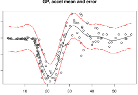
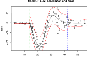
Figure 3: Motorcycle Dataset, fit (left) by a stationary process and right by our nonstationary model.

Figure 3 shows the data and the fits given by both a stationary GP (left) and the treed GP model (right), along with 90% credible intervals. For the treed GP, vertical lines illustrate a typical treed partition $\mathcal{T}$. Notice that the stationary GP is completely unable to capture the heteroscedasticity, and that the large variability in the central region drives both ends to be more wiggly (in particular, the transition from the flat left initial region requires an upward curve before descending). In contrast, the treed GP clearly reflects the differing levels of uncertainty, as well as allowing a flatter fit to the initial segment and a smoother fit to the final segment. 20,000 MCMC rounds yielded an average of 3.11 partitions in $\mathcal{T}$.

These results differ from those of Rasmussen & Ghahramani (2002). In particular, the error-bars they report for the leftmost region seem too large relative to the other regions. They use what they call an “infinite mixture of GP experts” which is a Dirichlet process mixture of GPs. They report that the posterior distribution uses between 3 and 10 experts to fit this dataset, with even 10-15 experts still having considerable posterior mass, although there are “roughly” three regions. Contrast this with the treed GP model which almost always partitions into three regions, occasionally four, rarely two. On speed grounds, the treed GP is also a winner. Running the mixture of GP experts model using a total of 11,000 MCMC rounds, discarding the first 1,000, took roughly one hour on a 1 GHz Pentium. Allowing treed GP to use 25,000 MCMC rounds, discarding the first 5,000, takes about 3 minutes on a 1.8 GHz Athalon.

We note that the mean fitted function in the right plot in Figure 3 is essentially that of a continuous function. Figure 4 shows examples of the fits from individual MCMC iterations that are eventually averaged. While the individual partition models are typically discontinuous, it is clear from Figure 3 that the mean fitted function is well-behaved.

Figure 4: Fits of the motorcycle accident data from individual MCMC iterations.

4.6 Limiting linear models

In some cases, a GP may not be needed within a partition, and a much simpler model, such as a linear model, may suffice. In particular, because of the linear mean function in our implementation of the GP, the standard linear model can be seen as a limiting case. The linear model is then more parsimonious, as well as much more computationally efficient. Use of a model-switching prior allows practical implementation. More details are available in Gramacy and Lee, (2008). The value of such an approach can be seen from the fit on the right side of Figure 3. The leftmost partition looks quite flat, and so could be fit just as well with a line rather than a GP. The center partition clearly requires a GP fit. The rightmost partition looks mostly linear, and would give a posterior which is a mix of a GP and linear model. Indeed, Figure 4 shows examples of the individual fits, and the leftmost section is nearly always flat, the rightmost section is often but not always flat, and the center section is typically curved but even there it can be essentially piecewise linear (the range parameter $d$ is estimated to be large, giving a nearly linear fit). Replacing the full GP with a linear model in a partition greatly reduces the computational resources required to update the model in that partition. Treed and non-treed Gaussian process with jumps to the limiting linear model are implemented in the tgp package on CRAN, and we take advantage of the full formulation in our analyses herein.

5 Rocket Booster Model Results

We fit our treed GP model to the rocket booster data using ten independent RJ-MCMC chains with 15,000 MCMC rounds each. The first 5,000 were discarded as burn-in, and every tenth thereafter was treated as a sample from the posterior distribution $\pi(\mathcal{T},\mbox{\boldmath$\theta$}|Z)$. In total, 10,000 samples were saved.

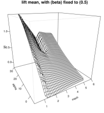
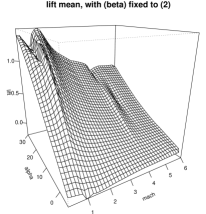
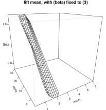
Figure 5: Posterior predictive mean surfaces of lift for all sideslip angles. Note that for levels 0.5 and 3 (center), Mach ranges only in $(1,5)$ and $(1.2,2.2)$

On a single 3.2 GHz Xeon processor this took about 60 hours. On the same machine, using the same (tuned) linear algebra libraries, inverting a single $3041\times 3041$ matrix takes about 17 seconds, so obtaining the same number of samples from a stationary GP would have taken a minimum of 708 hours. This is a gross underestimate because it assumes only one inverse is needed per MCMC round. Moreover, it does not count any of the $O(n^{2})$ operations like determinants of $\mathbf{K}$ (assuming a factorized $\mathbf{K}$ was saved in computing $\mathbf{K}^{-1}$) or multiplications like $\mathbf{Z}\mathbf{K}^{-1}\mathbf{Z}$ in (8), nor does it factor in the time needed to sample from the posterior predictive distribution.

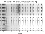
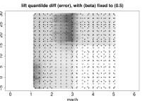
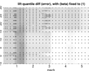
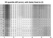
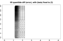
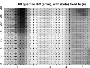
Figure 6: Posterior predictive variance surfaces of lift for all six sideslip angles. Dots show the locations of experimental runs. Darker shades are higher values.

Figures 5 & 6 summarize the posterior predictive distribution for the lift response for each of the six levels of sideslip angle. Figure 5 contains plots of the fitted mean lift surface by speed and angle of attack, and Figure 6 plots a measure of the estimated predictive uncertainty given by the difference in 95% and 5% quantiles of samples from the posterior predictive distribution. The treed GP works well here. Most of the space is nicely smooth, with the sharp transition at Mach one also well-modeled. Most of the potential false convergences have been smoothed out. But the estimated variability reflects both increased variability where the function is changing rapidly (e.g., near Mach one, particularly for higher sideslip levels) and especially where there are issues of possible false numerical convergence. Note that the uncertainty is not that high near Mach one at sideslip level zero because of the large number of samples taken in that region. We also note that the increased uncertainty seen in the top rows around Mach three and higher angles of attack is due to the noisy depression area in the data for sideslip level of one-half.

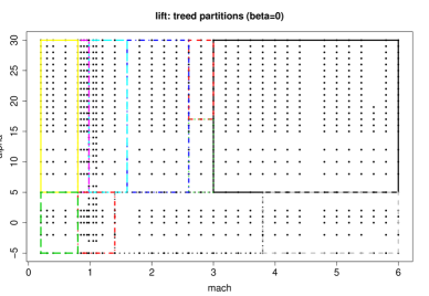
Figure 7: MAP treed partitions $\hat{\mathcal{T}}$ for the lift response at sideslip level zero.

Figure 7 shows the MAP treed partitions $\hat{\mathcal{T}}$ found during MCMC for the slice of sideslip level zero. Notice the aggressive partitioning near Mach one due to the regime shift between subsonic and supersonic speeds. Extra partitioning at low speeds and large angles of attack address the singularity outlined in Figure 1, and near Mach three due to the numerical instabilities at sideslip level one-half.

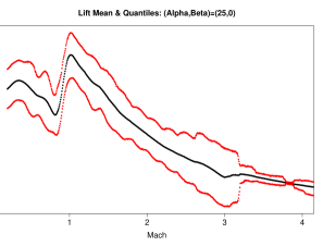
Figure 8: A slice of the mean fit with error bars as a function of Mach with alpha fixed to 25 and beta fixed to zero.

Figure 8 shows the mean fit and a 90% credible interval for once slice of predicting lift, with Mach on the $x$-axis and considering only angle of attack equal to 25 and slideslip angle equal to 0 (i.e., this is one slice from the upper left plot in Figure 5; this plot is from fitting the whole dataset, but we only plot one slice for visibility). The key item to note is that the fit is essentially continuous. The plot is made up only of points at fitted values, no interpolation or lines have been used.

Figure 9: Slices of the posterior predictive mean from individual MCMC iterations for the LGBB data with alpha fixed to 25 and beta fixed to zero.

In contrast, Figure 9 shows examples of the treed GP fits from individual MCMC iterations, which often have clear discontinuities from the partitioning structure. Thus as is typical, our mean fitted values are quite smooth, because they are an average, even though the individual components of the mean may not be continuous.

To measure goodness of fit we typically rely on qualitative visual barometers. For example, traces are used to asses mixing in the Markov chain, and posterior predictive slices and projections are inspected, as described above. For a more quantitative assessment we follow the suggestion of Gelfand, (1995) and use 10-fold cross validation. Posterior predictive quantiles are obtained for the input locations held-out of each fold, and the proportion of held-out responses that fall within the 90% predictive interval is recorded. For the LGBB data we found a proportion of 0.96 using the treed GP LLM model. Thus our model fits well, and if anything, our predictive intervals are slightly wider than necessary, so we appear to be fully accounting for uncertainty.

6 Conclusion

We developed the treed Gaussian process model for the rocket booster computer experiment, but it also has a wide range of uses as a simple and efficient method for nonstationary modeling. A fully Bayesian treatment of the treed GP model was laid out, treating the hierarchical parameterization of the correlation function $K(\cdot,\cdot)$ as a modular component, easily replaced by a different family of correlations. The limiting linear model parameterization of the GP can be both useful and accessible in terms of Bayesian posterior estimation and prediction, resulting in a uniquely nonstationary, semiparametric, tractable, and highly accurate model that contains the Bayesian treed linear model as a special case.

We believe that a large contribution of the treed GP will be in the domain of sequential design of computer experiments (Santner et al.,, 2003; Gramacy et al.,, 2004). Empirical evidence suggests that many computer experiments contain much linearity, as we have seen with large regions of the space for the rocket booster simulator. The Bayesian treed GP provides a full posterior predictive distribution (particularly a nonstationary and thus region-specific estimate of predictive variance) which can be used towards active learning in the input domain. Exploitation of these characteristics should lead to an efficient framework for the adaptive exploration of computer experiment parameter spaces.

References

- Abrahamsen, (1997) Abrahamsen, P. (1997). “A Review of Gaussian Random Fields and Correlation Functions.” Tech. Rep. 917, Norwegian Computing Center, Box 114 Blindern, N-0314 Oslo, Norway.
- Berger et al., (2001) Berger, J. O., de Oliveira, V., and Sansó, B. (2001). “Objective Bayesian Analysis of Spatially Correlated Data.” Journal of the American Statistical Association, 96, 456, 1361–1374.
- Breiman et al., (1984) Breiman, L., Friedman, J. H., Olshen, R., and Stone, C. (1984). Classification and Regression Trees. Belmont, CA: Wadsworth.
- Chipman et al., (1998) Chipman, H., George, E., and McCulloch, R. (1998). “Bayesian CART Model Search (with discussion).” Journal of the American Statistical Association, 93, 935–960.
- Chipman et al., (2002) — (2002). “Bayesian Treed Models.” Machine Learning, 48, 303–324.
- Cormen et al., (1990) Cormen, T. H., Leiserson, C. E., and Rivest, R. L. (1990). Introduction to Algorithms. The MIT EE & CS Series. MIT Press/McGraw Hill.
- Damian et al., (2001) Damian, D., Sampson, P. D., and Guttorp, P. (2001). “Bayesian Estimation of Semiparametric Nonstationary Spatial Covariance Structure.” Environmetrics, 12, 161–178.
- Denison et al., (2002) Denison, D., Adams, N., Holmes, C., and Hand, D. (2002). “Bayesian Partition Modelling.” Computational Statistics and Data Analysis, 38, 475–485.
- Denison et al., (1998) Denison, D., Mallick, B., and Smith, A. (1998). “A Bayesian CART Algorithm.” Biometrika, 85, 363–377.
- Fuentes, (2002) Fuentes, M. (2002). “Spectral Methods for Nonstationary Spatial Processes.” Biometrika, 89, 197–210.
- Gelfand, (1995) Gelfand, A. (1995). “Model Determination Using Sampling-Based Methods.” In Markov Chain Monte Carlo In Practice, eds. S. R. W. Gilks and D. Spiegelhalter, 145–161. London: Chapman Hall.
- Gilks et al., (1996) Gilks, W., Richardson, S., and Spiegelhalter, D. (1996). Markov Chain Monte Carlo in Practice. London: Chapman & Hall.
- Gramacy, (2005) Gramacy, R. B. (2005). “Bayesian Treed Gaussian Process Models.” Ph.D. thesis, University of California, Santa Cruz.
- Gramacy and Lee, (2008) Gramacy, R. B. and Lee, H. K. H. (2008). “Gaussian Processes and Limiting Linear Models.” Computational Statistics and Data Analysis, 53, 123–136.
- Gramacy et al., (2004) Gramacy, R. B., Lee, H. K. H., and Macready, W. (2004). “Parameter Space Exploration With Gaussian Process Trees.” In ICML, 353–360. Omnipress & ACM Digital Library.
- Higdon et al., (1999) Higdon, D., Swall, J., and Kern, J. (1999). “Non-Stationary Spatial Modeling.” In Bayesian Statistics 6, eds. J. M. Bernardo, J. O. Berger, A. P. Dawid, and A. F. M. Smith, 761–768. Oxford University Press.
- Hjort and Omre, (1994) Hjort, N. L. and Omre, H. (1994). “Topics in Spatial Statistics.” Scandinavian Journal of Statistics, 21, 289–357.
- Kennedy and O’Hagan, (2001) Kennedy, M. and O’Hagan, A. (2001). “Bayesian Calibration of Computer Models (with discussion).” Journal of the Royal Statistical Society, Series B, 63, 425–464.
- Kim et al., (2005) Kim, H.-M., Mallick, B. K., and Holmes, C. C. (2005). “Analyzing Nonstationary Spatial Data Using Piecewise Gaussian Processes.” Journal of the American Statistical Association, 100, 653–668.
- Matérn, (1986) Matérn, B. (1986). Spatial Variation. 2nd ed. New York: Springer-Verlag.
- Paciorek, (2003) Paciorek, C. (2003). “Nonstationary Gaussian Processes for Regression and Spatial Modelling.” Ph.D. thesis, Carnegie Mellon University, Pittsburgh, Pennsylvania.
- Rasmussen and Ghahramani, (2002) Rasmussen, C. and Ghahramani, Z. (2002). “Infinite Mixtures of Gaussian Process Experts.” In Advances in Neural Information Processing Systems, vol. 14, 881–888. MIT Press.
- Richardson and Green, (1997) Richardson, S. and Green, P. J. (1997). “On Bayesian Analysis of Mixtures With An Unknown Number of Components.” Journal of the Royal Statistical Society, Series B, Methodological, 59, 731–758.
- Rogers et al., (2003) Rogers, S. E., Aftosmis, M. J., Pandya, S. A., N. M. Chaderjian, E. T. T., and Ahmad, J. U. (2003). “Automated CFD Parameter Studies on Distributed Parallel Computers.” In 16th AIAA Computational Fluid Dynamics Conference. AIAA Paper 2003-4229.
- Sacks et al., (1989) Sacks, J., Welch, W. J., Mitchell, T. J., and Wynn, H. P. (1989). “Design and Analysis of Computer Experiments.” Statistical Science, 4, 409–435.
- Sampson and Guttorp, (1992) Sampson, P. D. and Guttorp, P. (1992). “Nonparametric Estimation of Nonstationary Spatial Covariance Structure.” Journal of the American Statistical Association, 87(417), 108–119.
- Santner et al., (2003) Santner, T. J., Williams, B. J., and Notz, W. I. (2003). The Design and Analysis of Computer Experiments. New York, NY: Springer-Verlag.
- Schmidt and O’Hagan, (2003) Schmidt, A. M. and O’Hagan, A. (2003). “Bayesian Inference for Nonstationary Spatial Covariance Structure via Spatial Deformations.” Journal of the Royal Statistical Society, Series B, 65, 745–758.
- R Development Core Team, (2004) R Development Core Team (2004). R: A language and environment for statistical computing. R Foundation for Statistical Computing, Vienna, Aus. ISBN 3-900051-00-3.
- Silverman, (1985) Silverman, B. W. (1985). “Some Aspects of the Spline Smoothing Approach to Non-Parametric Curve Fitting.” Journal of the Royal Statistical Society Series B, 47, 1–52.
- Stein, (1999) Stein, M. L. (1999). Interpolation of Spatial Data. New York, NY: Springer.
- Whaley and Petitet, (2004) Whaley, R. C. and Petitet, A. (2004). “ATLAS (Automatically Tuned Linear Algebra Software).”