The Pion Form Factor at Large Momentum Transfer
Abstract:
We present our calculations of the electromagnetic form factor of pions. We explore the properties of pion form factor at momentum transfer larger than previous studies by including more combinations of source and sink momenta and using more configurations.We fit our results using vector meson dominance (VMD) hypothesis.
1 Motivation
The pion form factor is often considered a good observable for studying the onset of the perturbative QCD (pQCD)regime in exclusive processes. There are several reasons: First, the asymptotic forms of the pion form factor at both large and small are known. At large it scales as [1, 2, 3, 4, 5, 6, 7, 8, 9]
| (1) |
while at small , the pion form factor can be well described by the Vector Meson Dominance (VMD) Model [10, 11, 12]
| (2) |
Therefore at some there must be a transition from the VMD behavior to the large scaling predicted by pQCD. Since the pion is the lightest hadron, the transition is expected to occur at lower than heavier hadrons, which makes it relatively easier to probe by both experiments and Lattice QCD (LQCD). Finally, there is no disconnected diagram on the lattice for the pion form factor. Thus the calculation is pretty straightforward. Previous LQCD studies on the pion form factor can be found in [13, 14, 15, 16] and the references therein.
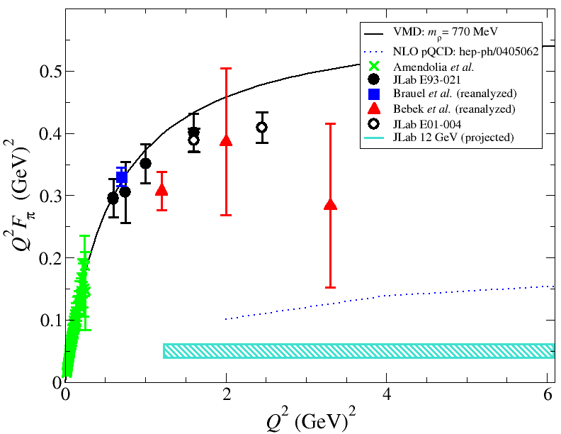
The current results from various experiments are shown in Fig. 1, including the latest results from Jefferson Lab (JLab) experiments E93-021 [17, 18] and E01-004 [19]. As we can indicate from the figure, the data points around start to show some hints of deviation from the VMD fit. This is the energy regime we would like to explore in our study.
2 Lattice Techniques
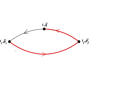
In this section we explain the techniques we used in our lattice calculations, namely the sequential source method (for calculating the quark propagator) and the ratio method (for the correlation functions). The pion electromagnetic form factor is obtained in LQCD by placing a pion creation operator (the “source”) at Euclidean time with momentum , a pion annihilation operator (the “sink”) at with momentum , and a current insertion at time with momentum transfer , as shown in Fig. 2. The standard quark propagator calculation provides the two propagator lines that originate from , the remaining propagator from is obtained by the sequential source method: completely specify the quantum numbers and at the sink, and contract the propagator from to with the annihilation operator to serve as the source vector of a second, sequential propagator inversion. The advantage of using the sequential source method is that various currents with different can be inserted at time without additional matrix inversions. The largest available lies in Breit frame ().
To obtain a simple expression on the lattice, we construct the pion form factor using the ratio method. The pion form factor is defined as
| (3) | |||
where is the chosen vector current. We can extract from some ratio of the three-point correlation function and the two-point functions. The three-point function can be written as
| (4) |
where ’s are operators with pion quantum numbers; and denote either “local”() or “smeared”(). Inserting complete sets of hadron states and requiring , gives
| (5) |
Similarly for the two-point correlator,
| (6) |
We can obtain from the following ratio
| (7) | |||||
where the indices , and can be either (local) or (smeared).
3 Simulation Details and Results
We use lattices generated by MILC [20], with volume and lattice spacing fm. The sea quark mass and the valence quark mass are tuned so that we get the same lightest pion mass [21]. The pion operators are fixed at time and , and the number of configurations used in this study is . We use five different sets of sink momenta: , and .
We present our results in terms of the square of the pion charge radius, obtained by the VMD fit:
| (8) |
as shown in Fig. 3. The first point on the left is from the data set with only zero sink momentum (), and for the next point we combined the data from both and , and for the third point we added in , and so on.
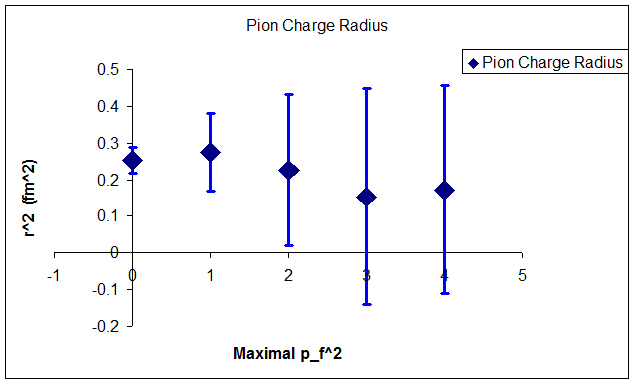
We can see from Fig. 3 that the error bars of increases as higher sink momenta are included. Since the pion charge radius is related to the slope of at low , we derive from the data set of zero sink momentum and , and check the consistency between the VMD fit and the data above to see if there is any deviation from the VMD model.
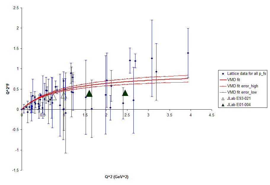
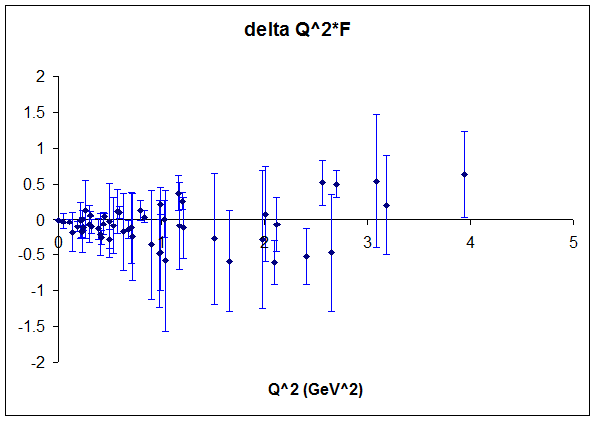
The result of this “consistency check” is presented in Fig. 4, where we plot against . While the quantity should approach a constant as predicted by VMD, we can see that there are some hints of deviation from the VMD model for points with . To further emphasize this observation, we define , and plot against in Fig. 5.
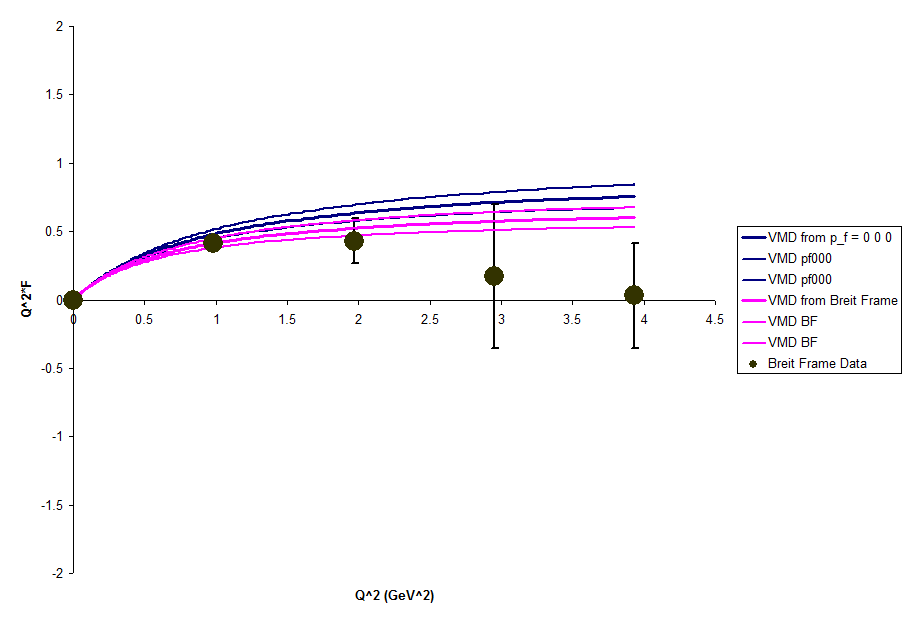
We also compared this VMD fits from low with that from the Breit frame (where), for the data points of the Breit frame have relatively small error bars at high . The result is shown in Fig. 6. The figure implies that the VMD fit from the Breit frame (the purple one) is about away from the fit of a single zero sink momentum (the blue one), hence exploring further in the Breit frame may be the correct direction for studying the pion form factor at higher momentum transfer.
4 Summary and Outlook
In this study we have acquired enough lattice data for to extract a reliable pion charge radius . By comparing the VMD fit from data with low and high , we’ve started to see some hints of discrepancy between data points at different momentum transfer, which may indicate the transition from the VMD model to pQCD, the goal we are seeking for. We also found that the VMD fit from the Breit frame is about away from the fit of a single zero sink momentum, and we infer that we may explore further in the high regime by studying the data from the Breit frame. We are generating four times more data to shrink the error bars in the Breit frame in the hope of a clearer and stronger evidence of the transition into the perturbative QCD regime.
In the meantime, the JLQCD Collaboration has also reported their calculation of the pion form factor based on all-to-all propagators. Interested readers may find details in their upcoming publication [22].
References
- [1] S. J. Brodsky and G. R. Farrar, Phys. Rev. Lett. 31, 1153 (1973).
- [2] S. J. Brodsky and G. R. Farrar, Phys. Rev. D 11, 1309 (1975).
- [3] G. R. Farrar and D. R. Jackson, Phys. Rev. Lett. 43, 246 (1979).
- [4] A. V. Radyushkin, arXiv:hep-ph/0410276.
- [5] A. V. Efremov and A. V. Radyushkin,in Proceedings of the XIX International Conference on High Energy Physics, Tokyo, Japan, August 23-30, 1978, edited by S. Homma(Physical Society of Japan,Tokyo,1979), jINR-E2-11535.
- [6] A. V. Efremov and A. V. Radyushkin, Theor. Math. Phys. 42, 97 (1980).
- [7] A. V. Efremov and A. V. Radyushkin, Phys. Lett. B 94, 245 (1980).
- [8] D. R. Jackson, Ph.D. thesis,California Institute of Technology (1977).
- [9] G. P. Lepage and S. J. Brodsky, Phys. Lett. B 87, 359 (1979).
- [10] W. G. Holladay, Phys. Rev. 101, 1198 (1956).
- [11] W. R. Frazer and J. R. Fulco, Phys. Rev. Lett. 2, 365 (1959).
- [12] W. R. Frazer and J. R. Fulco, Phys. Rev. 117, 1609 (1960).
- [13] F. D. R. Bonnet, R. G. Edwards, G. T. Fleming, R. Lewis and D. G. Richards [Lattice Hadron Physics Collaboration], Phys. Rev. D 72, 054506 (2005) [arXiv:hep-lat/0411028].
- [14] S. Hashimoto et al. [JLQCD Collaboration], PoS LAT2005, 336 (2006) [arXiv:hep-lat/0510085].
- [15] D. Brömmel et al., PoS LAT2005, 360 (2006) [arXiv:hep-lat/0509133].
- [16] D. Brömmel et al. [QCDSF/UKQCD Collaboration], Eur. Phys. J. C 51, 335 (2007) [arXiv:hep-lat/0608021].
- [17] J. Volmer et al., Phys. Rev. Lett. 86, 1713 (2001).
- [18] V. Tadevosyan et al., Phys. Rev. C 75, 055205 (2007).
- [19] T. Horn et al., Phys. Rev. Lett. 97, 192001 (2006).
- [20] C. W. Bernard et al., Phys. Rev. D 64, 054506 (2001) [arXiv:hep-lat/0104002].
- [21] Ph. Hägler et al. [LHPC Collaboration], arXiv:0705.4295 [hep-lat].
- [22] T. Kaneko et al. [JLQCD Collaboration], PoS LAT2007, 148 (2007).