Abstract

It is well know that the coronagraphic observations of halo CMEs are subject to projection effects. Viewing in the plane of the sky does not allow us to determine the crucial parameters defining geoeffectivness of CMEs, such as the velocity, width or source location. We assume that halo CMEs at the beginning phase of propagation have constant velocities, are symmetric and propagate with constant angular widths. Using these approximations and determining projected velocities and difference between times when CME appears on the opposite sides of the occulting disk we are able to get the necessary parameters. We present consideration for the whole halo CMEs from SOHO/LASCO catalog until the end of 2000. We show that the halo CMEs are in average much more faster and wider than the all CMEs from the SOHO/LASCO catalog.

1 Introduction

Space Weather is significantly controlled by coronal mass ejections (CMEs) which can affect the Earth in a different way. CMEs originating close to the central meridian, directed toward the Earth, excite the biggest scientific concern. In coronagraphic observations they appear as enhancement surrounding the entire occulting disk and they were called ‘halo CME’. Since the first identification by Howard et al. (1982) plenty of them were detected and now they are routinely recorded by the high sensitive SOHO/LASCO coronagraphs. In spite of large advantage over previous instruments, the SOHO/LASCO observations are still affected by a projection effect (Gopalswamy et al. 2000b). Viewing in the plane of the sky does not allow us to determine the crucial parameters defining geoeffectivness of CMEs, such as the velocity, width or source location. Prediction of the arrival of CME in the vicinity of Earth is critically important in space weather investigations. Basing on interplanetary shocks detected by Wind and the corresponding CMEs detected by SOHO, Gopalswamy et al. (2000a) developed and next (Gopalswamy, 2001) improved an empirical model to predict the arrival of CMEs at 1AU. The critical element affecting this model is the initial CME speed. The better prediction could be achieved if real initial velocities are used instead projected velocities determined from LASCO observations. Similarly, attempts made to estimate the projection effect based on the location of the solar source employ ad hoc assumptions on parameter such as the width of CMEs (Sheeley et al. 1999, Leblanc and Dulk, 2000). In the present paper we try to determine these crucial parameters defining geoeffectivness of CMEs, such as the velocity, width or source location. We assume that halo CMEs at the beginning phase of propagation have a constant velocities, are symmetric and propagate with constant angular widths. Using these approximations and determining projected velocities and difference between times when CME appears on the opposite sides of the occulting disk we are able to get necessary parameters. We present results for the whole halo CMEs from SOHO/LASCO catalog until the and of 2000.

2 The cone model of CME

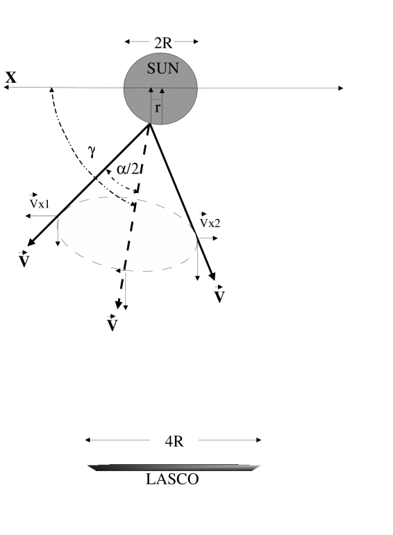
Figure 1: The schematic picture presenting our cone model of the halo CME.

Typical limb CMEs observed by the LASCO coronagraph look like ejected blobs of magnetized plasma with magnetic fields anchored to the sun surface. This allow them to keep almost cone shape during expansion through the C2 and C3 fields of view. The observed angular widths, for many limb events, remain nearly constant as a function of height (Webb et al. 1997, our founding during work on SOHO/LASCO catalog). Most of them propagate with constant radial frontal speed but many slow CMEs gradually accelerate and fast CMEs decelerate (St. Cyr et al., 2000; Sheeley et al 1999., Yashiro et al., 2002). Assuming that the halo CME propagate with a constant velocity and angular width we can reproduce it by the cone model with four free parameters such as the velocity, angular width and the orientation of the central axis. So we assume that bulk velocity of ejected blob is pointed radially and isotropically. In the Fig. 1. schematically we show the basic properties of our model. These assumptions should be true at the beginning phase of CME expansion at least. In the projection on the symmetry plane it looks like a triangle represented by solid thick arrows. The central axis of our CME is imaged by the dashed thick arrow. Its inclination to the plane of sky is equal $\gamma$. Each parts of this cone (triangle in projection) has a constant real velocity $V$. The CME with the angular width $\alpha$ is ejected from the Sun at distance $r$ from the central meridian. Opposite parts of CMEs have velocities, projected on the plane of sky, equal respectively $\vec{V}x1$ and $\vec{V}x2$. In the bottom of the picture we see the occulting disk of the LASCO/C2 coronagraph. We have to note that it is only schematic picture without a real scale. We may observe that if CME originates exactly in the center of the Sun it will appear at the same time around the entire occulting disk. But if the source location of CME is slightly shifted (=r)in respect to the center of the Sun (for example like in our picture) then CME will first appear at the left (east) side of the occulting disk and finally at the right (west) side of the occulting disk. Since this time we can see in the LASCO picture full halo CME ring but slightly asymmetric in respect to the occulting disk. The clue of this method is based on this asymmetry, in other words on the difference between times when CME appears at the opposite sides (first and finally appearance) of the occulting disk. Considering situation from our picture we can say that to see CME at the left (east) side of the occulting disk it has to travel, in the plane of sky, distance equal $2R-r$ with velocity $\vec{V}x1$. For this work CME needs time $T_{1}$ equal

$$T_{1}={(2R-r)\over\vec{V}x1}\qquad.$$

Similarly, CME will appear on the right (west) side of the occulting disk after time equal

$$T_{2}={(2R+r)\over\vec{V}x2}\qquad.$$

From these equations we determine the difference time

$$\Delta T=T_{2}-T_{1}={(2R+r)\over\vec{V}x2}-{(2R-r)\over\vec{V}x1}\qquad.$$

From the geometry of CME shown in the Fig. 1. we get the rest necessary equations

$$cos(\gamma)={r\over R}\qquad,$$

$$cos(\gamma-{\alpha\over 2})={Vx1\over V}\qquad.$$

$$cos(180^{o}-\gamma-{\alpha\over 2})={Vx2\over V}\qquad.$$

We have four equations and four parameters to determine $r$, $\alpha$, $V$ and $\gamma$. $Vx1$, $Vx2$ and $\Delta T$ we have to get from LASCO observations.

2.1 Determination parameters describing halo CMEs

Now we have to determine $Vx1$, $Vx2$ and $\Delta T$ from LASCO observations. It is not so easy because typically the halo CMEs are very faint and in addition their structure is very complicated. We consider the whole halo events from SOHO/LASCO catalog until the end of 2000. From LASCO observations we obtained two height-time plots for each halo CME from our sample. The first height-time plot is for this part of event which appears first from the occulting disk. It is extrapolated to estimate time ($T1$) when this part of CME, in the plane of sky, reaches heliocentric distance $=2R_{\odot}$ and to estimate velocity $Vx1$. The second height-time plot is used to determine the same parameters ($T2$ and $Vx2$) but in the opposite side of the occulting disk where the halo CME appears at last. An example of 1999/06/28 CME observed by LASCO is present in the Fig. 2 (figure is to big to see it in this archive). In the first panel at the time $T0$ we do not see any new event. In the next panel, in the north-west quadrant of the Sun, CME appears at time 07:31. From the height-time plot we determine $T1=07:19$ and $Vx1=635km/s$. In the next panel, the final part of CME appears in the south-west quadrant of the Sun. From this part we determined $T2=07:34$ and $Vx2=515km/s$. In the fourth panel we can see the full image of the halo CME at last. The thick solid arrow present the axis along which the respective parameters are determined. The position angle (PA = angle between north pole of the sun and part of the halo CME where the Vx1 is determined) is indicated also. So the difference time for this event will be $\Delta T=T2-T1=15min$. Now from equations (1, 2, 3 and 4) describing our CME model we can determine the $V$, width and parameter $r$.

3 Results

We made the same consideration for the rest events from our sample. The results are present in the three tables. Three first columns are got from the SOHO/LASCO catalog (date, time and projected speed from LASCO observations). Next, in four columns we have data received from our considerations of LASCO images ($PA,Vx1,Vx2,\Delta T$). Parameters estimated from our cone model $(r,\gamma,\alpha,V)$ are presented in columns 8,9,10 and 11. We also put, in a column 12, a short characteristic of a given event. Numbers from the range 0.0 until 3.0 describe quality of a given CME. The letter F informs that we have frontside, B backside and B? probably backside halo CME. If a halo CME is to faint to measure at list two hight-time points to determine velocity we could not estimate necessary parameters so we left empty space in our table and put quality $0$ in the column 12. Similarly, we could not determine the parameters for the symmetric halo CMEs. This situation appears when asymmetry in velocity is less than 10km/s minutes or in the difference time less than 10 minutes. In this case we put ‘Sym’ into column 12. In column 13, if it is possible, we identified the source location from GEOS X-flare onset.
DATE TIME SPEED PA Vx1 Vx2 $\Delta T$ r $\gamma$ $\alpha$ V Char Flare ${km\over s}$ Deg ${km\over s}$ ${km\over s}$ Min ${1\over R_{\odot}}$ Deg Deg ${km\over s}$ 1996/08/16 14:14:06 364 96 405 220 62 0.17 80 59 660 1.0,B? — 1996/11/07 23:20:05 497 114 412 361 18 0.16 80 133 429 1.0,B? — 1996/12/02 15:35:05 538 270 392 232 79 0.47 61 128 392 1.5,B? — 1997/01/06 15:10:42 136 182 100 85 75 0.13 82 105 117 0.5,F S20W03 1997/02/07 00:30:05 490 260 297 160 140 0.51 58 121 297 1.5,F S20W04 1997/04/07 14:27:44 875 126 956 551 23 0.42 65 139 954 2.0,F S30E19 1997/05/12 06:30:09 464 — — — — — — — — Sym N21W08 1997/07/30 04:45:47 104 276 94 85 81 0.25 75 146 95 1.0,B — 1997/08/30 01:30:35 405 65 397 163 103 0.21 78 56 590 1.0,F N30E17 1997/09/28 01:08:33 359 66 210 118 169 0.53 57 131 212 3.0,B — 1997/10/21 18:03:45 523 30 527 356 35 0.24 75 103 580 1.0,F N20E12 1997/10/23 11:26:50 503 — — — — — — — — 0.0,B — 1997/11/04 06:10:05 755 — — — — — — — — Sym S14W33 1997/11/06 12:10:41 1556 261 1524 765 34 0.82 34 153 2059 1.5,F S18W63 1997/11/17 08:27:05 611 — — — — — — — — Sym — 1997/12/18 23:47:31 417 68 321 270 40 0.36 68 158 325 2.5,B — 1998/01/02 23:28:20 438 258 281 142 197 0.93 20 165 602 2.0,B? — 1998/01/17 04:09:20 350 — — — — — — — — 0.0,B — 1998/01/21 06:37:25 361 176 387 265 80 0.71 44 159 468 0.5,F S57E19 1998/01/25 15:26:34 693 36 471 216 98 0.50 60 114 471 1.0,F N24E27 1998/03/29 03:48:00 1794 — — — — — — — — 0.0,B? — 1998/03/31 06:12:02 1992 167 1733 502 41 0.26 74 53 2591 3.0,B? — 1998/04/23 06:55:20 1618 113 1744 945 21 0.51 59 126 1744 3.0,F — 1998/04/27 08:56:06 1434 — — — — — — — — 0.0,F S16E50 1998/04/29 16:58:54 1374 16 1071 794 17 0.26 74 111 1134 2.0,F S17E20 1998/05/01 23:40:09 585 142 623 367 31 0.1 84 40 1427 2.0,F S18W05 1998/05/02 05:31:56 542 143 661 426 23 0.1 85 39 1612 2.0,F S20W17 1998/05/02 14:06:12 938 — — — — — — — — Sym S15W15 1998/06/04 02:04:45 1802 — — — — — — — — 0.0,B — 1998/06/05 12:01:53 320 223 170 109 215 0.78 39 159 227 1.0,F S23E43 1998/06/07 09:32:08 794 114 1117 834 17 0.4 66 143 1122 2.0,B — 1998/06/20 18:20:37 964 153 964 481 54 0.8 35 153 1285 2.0,B? — 1998/10/24 02:18:05 452 116 404 377 32 0.46 62 172 441 1.5,B? — 1998/11/04 04:54:07 527 0.0 390 158 114 0.25 75 62 541 1.5,F N17W01 1998/11/05 02:24:56 577 288 395 267 42 0.18 79 88 482 1.0,F N19W10 1998/11/05 20:58:59 1124 305 1092 378 55 0.35 69 75 1283 3.0,F N22W18 1998/11/24 02:30:05 1744 224 1856 628 43 0.88 27 153 2655 3.0,F S30W81 1998/11/26 03:42:05 488 — — — — — — — — 0.0 — 1998/12/18 18:21:50 1745 40 1758 532 50 0.68 47 120 1792 2.0,F N19E64 1999/04/04 04:30:07 1178 — — — — — — — — 0.0,F N18E72 1999/04/24 13:31:15 1495 307 1259 502 45 0.52 58 110 1261 2.0,B — 1999/05/03 06:06:05 1584 50 1392 345 61 0.61 51 110 1369 2.0,F N15E32

DATE	TIME	SPEED	PA	Vx1	Vx2	$\Delta T$	r	$\gamma$	$\alpha$	V	Char	Flare
		${km\over s}$	Deg	${km\over s}$	${km\over s}$	Min	${1\over R_{\odot}}$	Deg	Deg	${km\over s}$
1999/05/10	05:50:05	920	80	1080	513	33	0.27	74	76	1333	1.5,F	N16E19
1999/05/27	11:06:05	1691	311	1700	623	42	0.71	44	130	1821	1.5,B	—
1999/06/01	19:37:35	1772	351	1792	662	32	0.40	65	88	1902	1.5,B	—
1999/06/04	00:50:06	803	8	936	475	38	0.37	68	101	980	1.5,B?	—
1999/06/08	21:50:05	726	10	755	690	19	0.49	60	170	834	1.5,F	N30E03
1999/06/12	21:26:08	465	—	—	—	—	—	—	—	—	Sym	N22E37
1999/06/22	18:54:05	1133	—	—	—	—	—	—	—	—	0.0,F	N22E37
1999/06/23	06:06:05	450	—	—	—	—	—	—	—	—	Sym	S10E71
1999/06/23	07:31:24	1006	—	—	—	—	—	—	—	—	Sym	S12E78
1999/06/24	13:31:24	975	—	—	—	—	—	—	—	—	0.0,F	N29E13
1999/06/26	07:31:25	558	0	584	419	21	0.11	83	67	909	1.0,F	N25E00
1999/06/28	12:06:07	560	364	549	297	77	0.67	47	143	603	1.0,F	S27E55
1999/06/28	21:30:08	1083	—	—	—	—	—	—	—	—	0.0,F	S25E49
1999/06/29	05:54:06	589	—	—	—	—	—	—	—	—	0.0	—
1999/06/29	07:31:26	634	10	635	515	15	0.15	81	112	698	2.0,F	N18E07
1999/06/29	18:54:07	438	—	—	—	—	—	—	—	—	0.0,F	S14E01
1999/06/30	04:30:05	1049	—	—	—	—	—	—	—	—	0.0	—
1999/06/30	11:54:07	627	193	588	424	23	0.16	80	92	705	1.0,F	S15E00
1999/06/30	13:31:25	514	—	—	—	—	—	—	—	—	0.0	—
1999/07/06	17:06:05	899	350	1000	489	39	0.41	65	105	1026	1.0,B	—
1999/07/19	03:06:05	509	—	—	—	—	—	—	—	—	0.0,F	N15W13
1999/07/25	13:31:21	1389	306	1342	348	82	0.76	40	127	1466	2.0,F	N29W81
1999/07/28	05:30:05	457	—	—	—	—	—	—	—	—	0.0,F	S15E00
1999/07/28	09:06:05	456	—	—	—	—	—	—	—	—	0.0,F	S15E04
1999/08/07	23:50:05	219	—	—	—	—	—	—	—	—	0.0,F	S14E47
1999/08/09	03:26:05	369	—	—	—	—	—	—	—	—	0.0,F	S29W11
1999/10/14	09:26:05	1250	63	1362	830	33	0.82	34	157	1899	2.0,F	N15E40
1999/12/06	09:30:08	653	154	680	551	21	0.33	70	147	682	1.0,B?	—
1999/12/12	08:30:05	720	198	1118	797	21	0.50	59	147	1151	1.0,B	—
1999/12/20	18:06:05	1237	15	1237	783	23	0.28	73	74	2242	2.0,B	—
1999/12/22	02:30:05	482	14	753	525	42	0.75	40	162	984	1.5,F	N10E30
1999/12/22	19:31:22	605	24	605	515	44	0.65	69	141	1042	1.5,F	N24E19
2000/01/14	10:54:34	229	—	—	—	—	—	—	—	—	0.0,B	—
2000/01/18	17:54:05	739	—	—	—	—	—	—	—	—	0.0,F	S19E11
2000/01/25	23:54:06	222	—	—	—	—	—	—	—	—	0.0	—
2000/01/27	19:31:17	828	—	—	—	—	—	—	—	—	0.0,F	S09E71
2000/01/28	20:12:41	1177	—	—	—	—	—	—	—	—	0.0,F	S31W17
2000/02/03	12:30:05	735	—	—	—	—	—	—	—	—	0.0,B	—
2000/02/08	09:30:05	1079	55	938	732	28	0.63	50	162	1091	2.0,F	N25E26
2000/02/09	19:54:17	910	218	1124	693	25	0.44	63	128	1125	1.5,F	S17W40
2000/02/11	21:08:06	498	—	—	—	—	—	—	—	—	0.0	—
2000/02/12	04:31:20	1107	—	—	—	—	—	—	—	—	0.0,F	N26W23
2000/02/17	20:06:05	600	196	660	540	23	0.39	67	152	668	2.0,F	S27W10
2000/02/28	10:54:05	404	279	466	370	43	0.3	72	132	475	2.0,B?	—

DATE	TIME	SPEED	PA	Vx1	Vx2	$\Delta T$	r	$\gamma$	$\alpha$	V	Char	Flare
		${km\over s}$	Deg	${km\over s}$	${km\over s}$	Min	${1\over R_{\odot}}$	Deg	Deg	${km\over s}$
2000/03/01	03:30:05	529	217	628	488	38	0.64	49	162	737	2.0,B?	—
2000/03/03	05:30:07	793	—	—	—	—	—	—	—	—	0.0,F	S14W62
2000/03/29	10:54:30	949	—	—	—	—	—	—	—	—	0.0,B	—
2000/04/04	16:32:37	1188	304	1281	641	40	0.79	37	151	1645	2.0,F	N16W66
2000/04/10	00:30:05	383	—	—	—	—	—	—	—	—	0.0,F	S14W01
2000/04/23	12:54:05	1187	279	1309	533	46	0.65	49	127	1351	3.0,B	—
2000/05/03	02:06:05	693	—	—	—	—	—	—	—	—	Sym,B	—
2000/05/05	15:50:05	1594	269	1624	570	50	0.85	32	146	2154	2.0,F	S16W84
2000/05/12	23:26:05	2604	63	2056	699	36	0.62	51	116	2072	2.0,B	?—
2000/05/28	11:06:05	572	—	—	—	—	—	—	—	—	0.0,B?	—
2000/06/02	10:30:25	442	—	—	—	—	—	—	—	—	0.0,F	N10E23
2000/06/06	15:54:05	1108	6	1024	870	12	0.32	71	152	1028	2.5,F	N21E15
2000/06/07	16:30:05	842	—	—	—	—	—	—	—	—	0.0,F	N20E02
2000/06/10	17:08:05	1108	306	1376	710	32	0.64	50	138	1460	2.5,F	N22W37
2000/07/07	10:26:05	453	198	311	239	59	0.42	65	147	315	1.5,B?	—
2000/07/11	13:27:23	1078	51	1453	1093	18	0.68	47	162	1753	2.0,F	N18E27
2000/07/14	10:54:07	1674	—	—	—	—	—	—	—	—	0.0,F	N22E07
2000/07/27	19:54:06	905	—	—	—	—	—	—	—	—	0.0,F	N10E07
2000/08/09	16:30:05	702	—	—	—	—	—	—	—	—	0.0,F	N11W09
2000/09/12	11:54:05	1550	216	1250	966	18	0.58	54	159	1385	2.0,F	S12W18
2000/09/12	17:30:05	1053	47	1329	681	27	0.39	66	106	1366	2.0,B?	—
2000/09/15	15:26:05	481	—	—	—	—	—	—	—	—	0.0,F	N14E02
2000/09/15	21:50:07	257	—	—	—	—	—	—	—	—	0.0,F	N14E01
2000/09/16	05:18:14	1251	21	1256	946	12	0.27	74	126	1278	2.0,F	N14E04
2000/09/25	02:50:05	587	—	—	—	—	—	—	—	—	0.0,F	N15W28
2000/10/02	03:50:05	525	144	577	381	42	0.41	65	131	578	1.0,F	S08E05
2000/10/02	20:26:05	569	—	—	—	—	—	—	—	—	0.0,F	S08E05
2000/10/09	23:50:05	798	—	—	—	—	—	—	—	—	0.0,F	N02W18
2000/11/01	16:26:08	801	—	—	—	—	—	—	—	—	0.0,F	S17E39
2000/11/03	18:26:06	291	—	—	—	—	—	—	—	—	0.0,F	N02W02
2000/11/08	04:50:23	474	236	622	294	77	0.6	53	128	634	1.0,F	N10W77
2000/11/08	23:06:05	1345	—	—	—	—	—	—	—	—	0.0,F	N05W75
2000/11/15	23:54:05	826	—	—	—	—	—	—	—	—	0.0,B	—
2000/11/23	06:06:05	492	230	450	334	48	0.49	60	150	466	1.0,F	S22W33
2000/11/24	05:30:05	1074	352	996	734	21	0.45	62	147	1013	1.5,F	N22W02
2000/11/24	15:30:05	1245	324	1396	841	17	0.26	74	96	1556	3.0,F	N22W07
2000/11/24	22:06:05	1005	312	1105	575	37	0.56	55	130	1122	2.0,F	N21W14
2000/11/25	01:31:58	2519	75	2434	724	34	0.54	57	100	2452	2.0,F	N07E50
2000/11/25	09:30:17	675	—	—	—	—	—	—	—	—	0.0,B?	—
2000/11/25	19:31:57	671	—	—	—	—	—	—	—	—	0.0,F	N20W23
2000/11/26	17:06:05	1026	283	1240	785	25	0.58	54	144	1303	2.0,F	N18W38
2000/12/06	17:26:05	413	—	—	—	—	—	—	—	—	Sym,B	—
2000/12/18	11:50:05	510	—	—	—	—	—	—	—	—	0.0,F	N14E03
2000/12/28	12:06:05	930	—	—	—	—	—	—	—	—	Sym,B	—

3.1 Properties of the halo CMEs

In the three tables we present list of the halo CMEs covering period of time from August 1996 until the end of 2000. We have to note that not all halo CMEs look identical. We have to consider two types of halo CMEs. First, the classical full halo CMEs which appear to surround the occulting disk very fast in the C2 LASCO coronagraph. Generally they originate from close the disk center. Second, the wide limb CMEs which surround the entire occulting disk very late, often in the field of view of the C3 LASCO coronagraph. Sometimes limb events appears as halo due to deflections of pre-existing coronal structures by the fast CME. So we have to be very careful to distinguish between a real halo CME and a limb fast event deflecting coronal material. We were able to determine the respective parameters for 73th CMEs from our sample. The rest CMEs had to more complicated structures, were to faint or symmetric and it was to difficult to accomplish necessary measurements. In the three histograms (Fig. 3, Fig. 4, Fig. 5) we present distribution of $V$, $\alpha$, and $\gamma$. Here it is important to note the halo CMEs seem to be much wider and faster than typical events taken from the SOHO/LASCO catalog (Yashiro et al. 2002). The average wide of halo CME is approximately equal 120^o (more than two times that the value received from the SOHO/LASCO catalog). The narrowest CME has width equal $40^{o}$ and the widest one has the cone angle as large as $172^{o}$. The average speed of the halo CMEs is $1080km/s$ (abut two times more than the one from SOHO/LASCO catalog). The slowest one achieves velocity equal $95km/s$ when the fastest is ejected with velocity $2590km/s$. Fig. 5 show that the halo CMEs originate close to the sun center (with $\gamma\geq 60^{o}$ ) with maximum of distribution around $\gamma=65^{o}$. We have to remember that in our consideration the symmetric CMEs which start exactly from the sun center are not included. If we consider them the maximum of $\gamma$ distribution could be shifted to the central meridian. In the Fig. 6 we present the sky plane speeds against corrected (real) velocities. The solid line represents linear fit to the data points. The inclination of the linear fit suggests that the projection effect slightly increases with speed of CMEs. It is clear that the projection effect is important and in average the corrected speeds are 20 percents larger than the velocities measured in the plane of sky.

4 Summary

In this paper we present possibility to estimate the crucial parameters determining geoeffectiveness of the halo CMEs. The clue of this method is based on the difference between times when the halo CME appears at the opposite sides (first and finally appearance) of the occulting disk. We considered the whole events form SOHO/LASCO catalog until the end of 2000. We were able to determine the real velocity, width and source location for 73th CMEs from our sample. Unfortunately, 58 events were symmetric or too faint to do necessary considerations. Results are listed in the three successive tables. This list could be use for further statistical examination or to prediction of the arrival of CME in the vicinity of Earth. Presented results suggest that the halo CMEs represent a specific class of CMEs which are very wide and fast. Using our results we have to remember that the simple model has several shortcomings: (i) CMEs may be accelerating, moving with constant speed or decelerating at the beginning phase of propagation. This means the constant velocity we assumed may not hold. (ii) CMEs may expand in addition to radial motion. Then the measured sky-plane speed is a sum of the expansion speed and the projected radial speed. This also would imply that the CMEs may not be a rigid cone as we assumed (Gopalswamy et al. 2001) (iii) The cone symmetry also may not hold. CME originating from loop structure could be elongated. All these limits can be overcome by stereoscopic observations only. Unfortunately, at the present time they are not available yet. It is necessary to develop the model to get the better fit to observations. The first step to improve our model could be achieved by consideration of acceleration and expansion of CMEs.

Acknowledgments
This paper was done during work of Grzegorz Michalek at Center for Solar and Space Weather, Catholic University of America in Washington.
In this paper we used data from SOHO/LASCO CME catalog. This CME catalog is generated and maintained by the Center for Solar Physics and Space Weather, The Catholic University of America in cooperation with the Naval Research Laboratory and NASA. SOHO is a project of international cooperation between ESA and NASA.
Work done by Grzegorz Michalek was partly supported by Komitet Badań Naukowych through the grant PB 258/P03/99/17.

References

Gopalswamy, N., et al., Geophys. Res. Lett., 27, 145, 2000a
Gopalswamy, N., et al., Geophys. Res. Lett., 27, 1427, 2000b
Gopalswamy, N., et al., J. Geophys. Res., 106, 292907, 2001
Gopalswamy, N., 2001 Coronal Mass ejection:Initiation and Detection?????
Howard R.A., et al., Astrophys. J., 263, L101, 1982
Leblanc, Y., Dulk, G.A., J. Geophys. Res., 106, 25301, 2001
Sheeley, N.R., Jr., Walters, J.H., Wang, Y.-M., Howard, R.A., J. Geophys.
          Res., 104, 24739, 1999
St. Cyr, O.C., et al., J. Geophys. Res., 105, 18169, 2000
Webb, D.F., et al., J. Geophys. Res., 102, 24161, 1997
Yashiro, S., et al.,in preparation, 2002

Figure 2: The histogram showing distribution of $V$ for the halo CMEs.

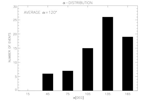
Figure 3: The histogram showing distribution of $\alpha$ for the halo CMEs.

Figure 4: The histogram showing distribution of $\gamma$ for the halo CMEs.

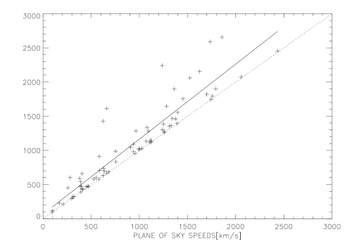
Figure 5: The plane of the sky speeds against the corrected (real) speeds. The solid line shows the linear fit to data