The piston dispersive shock wave problem

Abstract

The one-dimensional piston shock problem is a classical result of shock wave theory. In this work, the analogous dispersive shock wave (DSW) problem for a dispersive fluid described by the nonlinear Schrödinger equation is analyzed. Asymptotic solutions are calculated using Whitham averaging theory for a ”piston” (step potential) moving with uniform speed into a dispersive fluid at rest. These asymptotic results agree quantitatively with numerical simulations. It is shown that the behavior of these solutions is quite different from their classical counterparts. In particular, the shock structure depends on the speed of the piston. These results have direct application to Bose-Einstein condensates and the propagation of light through a nonlinear, defocusing medium.

The study of dispersive shock waves (DSWs) has gained interest with the recent experimental realization of DSWs in a Bose-Einstein condensate (BEC) Dutton et al. (2001); Hoefer et al. (2006) and the propagation of light through a nonlinear, defocusing medium Wan et al. (2007). Comparisons between classical, viscous shock waves (VSWs) and DSWs have been discussed in the context of single shocks Hoefer et al. (2006) and the interaction of two shocks Hoefer and Ablowitz (2007) yielding some appealing similarities but also important differences. Motivated by the classical VSW piston problem, here we consider the generation of a DSW by a piston moving into a dispersive fluid at rest.

The theoretical study of DSWs involves averaging a periodic wave over its period and allowing for slow variation of the wave’s parameters. This method, known as Whitham averaging Whitham (1965), has been successfully applied to many DSW problems including step initial data for the nonlinear Schrödinger (NLS) equation Gurevich and Krylov (1987); El et al. (1995), Bose-Einstein condensates Kamchatnov et al. (2004); Hoefer et al. (2006), fiber optics Kodama (1999), the generation of ultrashort lasers Biondini and Kodama (2006), and DSW interactions Hoefer and Ablowitz (2007). We also note that a dispersive piston shock problem arises as an asymptotic reduction of 2D, supersonic flow of a dispersive fluid around an obstacle El et al. (2004).

The piston shock problem is one of the canonical problems in the theory of VSWs. A uniform gas is held at rest in a long, cylindrical chamber with a piston at one end. When the piston is impulsively moved into the gas with constant speed, a region of higher density builds up between the piston and a shock front which propagates ahead of it. An elegant asymptotic solution to this problem is well known and relates the shock speed to the speed of the piston and the initial density of the gas (see e.g. Courant and Friedrichs (1948) and the discussion at the end of this work).

In this work, we consider the problem of a “piston” moving with constant speed into a steady, dispersive fluid: e. g. a Bose-Einstein condensate or light propagating through a nonlinear, defocusing medium. The piston in this case is a step potential that moves with uniform velocity. This potential could be realized in a BEC with a repulsive dipole beam and in nonlinear optics with a local change in the index of refraction. One expects, in analogy with the classical, viscous case, the generation of a dispersive shock wave. As we will show, this is indeed the case. There are two types of asymptotic behavior depending on the piston velocity. For smaller piston velocities, a region of larger density or intensity builds up between the piston and a DSW. However, for large enough piston velocities, a locally periodic wave is generated between the piston and the DSW which has no VSW correlate. The asymptotic results are verified by numerical simulations demonstrating quantitative agreement.

We consider the 1D NLS equation with a potential (also known as the Gross-Pitaevskii (GP) equation)

$$i\varepsilon\Psi_{t}=-\frac{\varepsilon^{2}}{2}\Psi_{xx}+V_{0}(x,t)\Psi+|\Psi|^{2}\Psi,\quad 0<\varepsilon\ll 1.$$ (1)

This equation models the mean field of a quasi-1D BEC Perez-Garcia et al. (1998) and the slowly varying envelope of the electromagnetic field propagating through a Kerr medium Boyd (2003) (where time $t$ is replaced by the propagation distance). The small parameter $\varepsilon$ is inversely proportional to the number of atoms in the BEC Hoefer et al. (2006) or, after rescaling, inversely proportional to the maximum initial intensity of the electromagnetic field. For all calculations in this work, we assume $\varepsilon=0.015$, a typical experimental value for BEC Hoefer et al. (2006). The piston problem is modeled with a temporally and spatially varying step potential given by

$$\begin{split}V_{0}(x,t)&=V_{max}H(v_{p}t-x),\quad H(y)=\left\{\begin{array}[]{cc}0&y<0\\ 1&y\geq 0\end{array}\right.,\end{split}$$

with strength $V_{max}$ and constant velocity $v_{p}$. The initial conditions are

$$\Psi(x,0)\to\sqrt{\rho_{R}}~{}\textrm{as}~{}x\to\infty,\quad\Psi(x,0)\to 0~{}\textrm{as}~{}x\to-\infty.$$

Because the strength of the piston is large, $V_{max}\gg\rho_{R}$, the density/intensity rapidly decay to zero near the origin. We assume that the wavefunction $\Psi$ is in the ground state of the step potential $V_{max}H(-x)$ when $t\leq 0$. For all calculations in this work, $\rho_{R}=0.133$.

It is useful to view eq. (1) in its hydrodynamic form by making the transformation $\Psi=\sqrt{\rho}e^{\frac{i}{\varepsilon}\int_{0}^{x}u(x^{\prime},t)\,\mathrm{d}x^{\prime}}$ and inserting this expression into the first two local conservation equations for the GP equation

$$\begin{split}\rho_{t}+(\rho u)_{x}&=0\\[5.69054pt] (\rho u)_{t}+\left(\rho u^{2}+\tfrac{1}{2}\rho^{2}\right)_{x}&=\frac{\varepsilon^{2}}{4}(\rho(\log\rho)_{xx})_{x}-\rho V_{0_{x}},\end{split}$$ (2)

where $\rho$ is the dispersive fluid “density” and $u$ is the dispersive fluid “velocity”. These equations are similar to the Navier-Stokes (NS) equations of fluid dynamics except that the viscous term of NS has been replaced by the dispersive term with coefficient $\varepsilon^{2}/4$.

Because the dispersive term in eq. (2) is small, one expects the generation of small wavelength $O(\varepsilon)$ oscillations near a steep gradient in the fluid variables. Witham’s method is to average an exact periodic solution over fast oscillations and assume that the wave’s parameters (amplitude, frequency, wavelength, etc.) vary slowly Whitham (1965).

We convert the piston DSW problem into a moving boundary value problem where appropriate boundary conditions are imposed at the piston front. First we solve the piston DSW problem assuming sufficiently small, positive piston velocities $v_{p}$. “Small” will be defined below.

We assume the piston strength is large for $x<v_{p}t$, so there is negligible density there. Assuming there is a jump from zero density to the nonzero value $\rho_{L}$ with a fluid velocity $u_{L}$ we integrate the first conservation law in eqs. (2) across the jump to find

$$-v_{p}\rho_{L}+\rho_{L}u_{L}=0.$$ (3)

This gives the first boundary condition at the piston

$$u(v_{p}t,t)\equiv u_{L}=v_{p},$$ (4)

the fluid velocity at the piston equals the piston velocity. We require a boundary condition for the density.

The theory of DSWs involves a system of quasi-linear, first order, hyperbolic equations known as the Whitham modulation equations. The Whitham equations describe the slow evolution of a periodic wave’s parameters and must be solved in order to find the asymptotic DSW solution. The simplest, non-trivial solutions to these equations are known as simple waves where only one dependent variable is varying in space and time, and the rest are constant. In analogy with gas dynamics, we assume a simple wave solution, but in this case to the Whitham equations. This determines a density $\rho_{L}$ at the piston. In order to connect to the uniform state ahead of the piston $\rho_{R}<\rho_{L}$, we must have a single DSW for $v_{p}$ sufficiently small ($v_{p}<2\sqrt{\rho_{R}}$). As we will show below, a “vacuum state” is created when $v_{p}\geq 2\sqrt{\rho_{R}}$, and we find a uniform traveling wave (TW) with speed $v_{p}$, instead of the constant density $\rho_{L}$, adjacent to the DSW. Later we verify with numerical simulations that these assumptions are reasonable. Now we derive the asymptotic piston DSW.

At the time $t=0^{+}$, we assume that there is a discontinuity in the fluid variables due to the impulsive motion of the piston at $t=0$

$$\rho(x,0^{+})=\left\{\begin{array}[]{cc}\rho_{L}&x=0\\ \rho_{R}&x>0\end{array}\right.,~{}u(x,0^{+})=\left\{\begin{array}[]{cc}u_{L}=v_{p}&x=0\\ u_{R}=0&x>0\end{array}\right..$$ (5)

This discontinuity is regularized by a slowly modulated, traveling wave, periodic solution to eq. (2) with $V(x,t)\equiv 0$ Gurevich and Krylov (1987)

$$\begin{split}\rho(x,t,\theta)&=\lambda_{3}-[\lambda_{3}-\lambda_{1}]\text{dn}^{2}(\theta;m),~{}m=\frac{\lambda_{2}-\lambda_{1}}{\lambda_{3}-\lambda_{1}}\\ u(x,t,\theta)&=V-\sigma\frac{\sqrt{\lambda_{1}\lambda_{2}\lambda_{3}}}{\rho(x,t,\theta)},~{}\sigma=\pm 1,~{}0<\lambda_{1}<\lambda_{2}<\lambda_{3}\\ \frac{\partial\theta}{\partial x}&=\sqrt{\lambda_{3}-\lambda_{1}}/\varepsilon,~{}\frac{\partial\theta}{\partial t}=-V\sqrt{\lambda_{3}-\lambda_{1}}/\varepsilon,\\ \end{split}$$ (6)

where the parameters $\lambda_{i}$, $i=1,2,3$ and $V$ satisfy

$$\begin{split}\lambda_{1}=&\tfrac{1}{16}(r_{1}-r_{2}-r_{3}+r_{4})^{2},~{}\lambda_{2}=\tfrac{1}{16}(-r_{1}+r_{2}-r_{3}+r_{4})^{2},\\ \lambda_{3}=&\tfrac{1}{16}(-r_{1}-r_{2}+r_{3}+r_{4})^{2},~{}V=\tfrac{1}{4}(r_{1}+r_{2}+r_{3}+r_{4}),\end{split}$$ (7)

and $r_{i}=r_{i}(x,t)$ evolve according to the Whitham equations

$$\begin{split}\frac{\partial r_{i}}{\partial t}+v_{i}(r_{1},r_{2},r_{3},r_{4})\frac{\partial r_{i}}{\partial x}=0,\quad i=1,2,3,4.\end{split}$$

The velocities $v_{i}$ are expressed in terms of complete elliptic integrals of the first and second kind Gurevich and Krylov (1987).

In order to find a simple wave solution to the Whitham equations, we require that only one of the parameters $r_{i}$ spatially varies and that the initial data for all the parameters $r_{i}$ properly characterizes the initial data in eq. (5) with the spatial average of eq. (6). We use the method of initial data regularization Kodama (1999); Biondini and Kodama (2006); Hoefer et al. (2006); Hoefer and Ablowitz (2007) to find

$$\begin{split}r_{1}&\equiv-2\sqrt{\rho_{R}},~{}r_{2}\equiv 2\sqrt{\rho_{R}},~{}r_{4}\equiv 2v_{p}+2\sqrt{\rho_{R}},\\ &r_{3}(x,0^{+})=\left\{\begin{array}[]{cc}2\sqrt{\rho_{R}}&x=0\\ 2v_{p}+2\sqrt{\rho_{R}}&x>0\end{array}\right.,~{}\sigma\equiv 1,\\ &\rho(v_{p}t,t)\equiv\rho_{L}=(\frac{1}{2}v_{p}+\sqrt{\rho_{R}})^{2}.\end{split}$$ (8)

The last equation, the boundary condition for the density at the piston, comes from the simple wave assumption. Equations (8) give rise to a self similar solution for $r_{3}$ satisfying the implicit relation

$$v_{3}(r_{1},r_{2},r_{3}(x,t),r_{4})=x/t.$$ (9)

Using a nonlinear root finder, eq. (9) is solved numerically for each $x$ and $t$. The values for $r_{i}$, $i=1,2,3,4$ are inserted into eqs. (7) and (6) to determine the asymptotic DSW solution. A pure DSW propagates ahead of the piston with trailing and leading edge speeds respectively Gurevich and Krylov (1987); Hoefer et al. (2006)

$$v_{s}^{-}=\frac{1}{2}v_{p}+\sqrt{\rho_{R}},~{}v_{s}^{+}=\frac{2v_{p}^{2}+4v_{p}\sqrt{\rho_{R}}+\rho_{R}}{v_{p}+\sqrt{\rho_{R}}}.$$ (10)

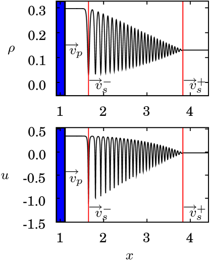
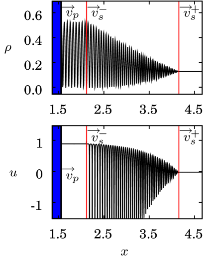
Figure 1: LEFT: Asymptotic piston DSW solution at time $t=3$ for $v_{p}=\sqrt{\rho_{R}}=0.365$. The vertical lines mark the left and right edges of the DSW moving with speeds $v_{s}^{-}=0.548$ and $v_{s}^{+}=1.278$ respectively. RIGHT: Asymptotic piston DSW solution at time $t=1.7$ when $v_{p}=2.5\sqrt{\rho_{R}}=0.912$. A locally periodic region connects the piston to the trailing edge of the DSW. The density minima in this region are approximately zero and the velocity is, theoretically, undefined (infinite) at these points. The density maxima are $4\rho_{R}=0.532$. DSW speeds are $v_{s}^{-}=1.245$, $v_{s}^{+}=2.452$.

Figure 1, left depicts the asymptotic piston DSW solution for a small piston velocity. The minimum values of the density and velocity occur at the trailing edge of the DSW and are Gurevich and Krylov (1987); Hoefer et al. (2006)

$$\rho_{min}=(\sqrt{\rho_{R}}-\frac{1}{2}v_{p})^{2},~{}u_{min}=-v_{p}(\frac{\sqrt{\rho_{R}}+\frac{1}{2}v_{p}}{\sqrt{\rho_{R}}-\frac{1}{2}v_{p}}).$$ (11)

The maximum values occur between the piston and the DSW: $\rho_{max}=\rho_{L}=(v_{p}/2+\sqrt{\rho_{R}})^{2}$, $u_{max}=u_{L}=v_{p}$ .

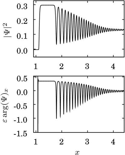
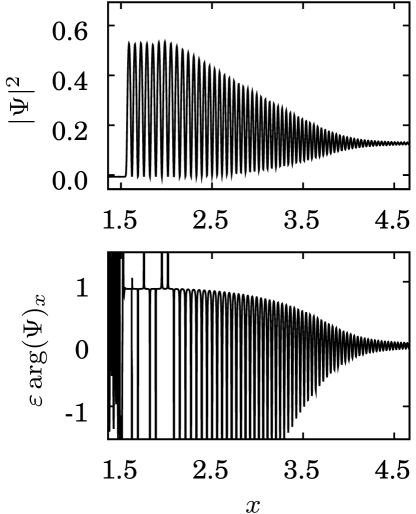
Figure 2: Numerical solutions to eq. (1) for the piston problem. LEFT: The density (upper) and velocity (lower) for the same parameters as in Fig. 1 LEFT. Numerically calculated trailing edge speed is $0.557$, approximately the theoretical value $0.548$. RIGHT: The density (upper) and velocity (lower) for the same parameters as in Fig. 1 RIGHT. Numerically calculated TW velocity of locally periodic wave is $0.912$, approximately the piston speed $0.913$.

It is possible for the piston velocity to be greater than the trailing DSW velocity calculated using eq. (10)

$$v_{p}\geq v_{s}^{-}\quad\text{if}\quad v_{p}\geq 2\sqrt{\rho_{R}}.$$

When $v_{p}=2\sqrt{\rho_{R}}$, $\rho$ can vanish (there is a so-called vacuum point) and a modification of the solution is required. To find a simple wave solution for large piston velocities, we must derive new conditions for the parameters $r_{i}$. We modify the DSW solution by introducing a locally periodic TW between the piston and the trailing edge of the DSW. When $v_{p}=2\sqrt{\rho_{R}}$, the DSW forms a vacuum point El et al. (1995); Hoefer et al. (2006) at the piston. The vacuum condition, $\rho=0$, is satisfied in eq. (6) when

$$\lambda_{1}=0~{}\Rightarrow~{}r_{1}-r_{2}-r_{3}+r_{4}=0~{}\Rightarrow~{}r_{4}-r_{3}=4\sqrt{\rho_{R}}.$$ (12)

Note that the fluid velocity is undefined at a vacuum point, even though the vacuum points have a well-defined propagation speed through the fluid. We assume that this condition holds for $v_{p}>2\sqrt{\rho_{R}}$ as well. One more condition is required to completely determine $r_{4}$ and $r_{3}(x=0,t=0^{+})$; $r_{1}$, $r_{2}$, and $r_{3}(x>0,0^{+})$ are determined by the initial data (5). Because there is a locally periodic TW between the piston and DSW, we assume that the velocity of the TW equals the piston velocity. This is the TW velocity condition

$$V=v_{p}~{}\Rightarrow~{}r_{1}+r_{2}+r_{3}+r_{4}=4v_{p}~{}\Rightarrow~{}r_{3}+r_{4}=4v_{p}.$$ (13)

Given the initial data in eq. (5) and the two conditions (12) and (13), only $r_{3}$ and $\sigma$ in the initial data of eq. (8) are altered

$$r_{3}(x,0^{+})=2v_{p}\mp 2\sqrt{\rho_{R}},~{}\sigma(x,0^{+})=\mp 1,~{}x\genfrac{}{}{0.0pt}{2}{=}{>}0.$$

Note that $\sigma=-1$ in the locally periodic region. Figure 1, right depicts the asymptotic DSW solution for $v_{p}>2\sqrt{\rho_{R}}$.

Several properties of this DSW solution are worth noting. The density between the piston and the DSW oscillates between the values

$$\rho_{min}=0\quad\text{and}\quad\rho_{max}=4\rho_{R},$$ (14)

independent of the piston velocity $v_{p}$ and the TW in this region propagates with the velocity $V=v_{p}$. Note that since the vacuum condition (12) holds everywhere inside the TW trailing the DSW, the velocity in this region, from eq. (6), is $u=V=v_{p}$ everywhere (except at the vacuum points where the velocity is undefined). The wavelength of the TW is $l=\frac{2\varepsilon}{v_{p}}K(4\rho_{R}/v_{p}^{2})$, where $K(m)$ and $E(m)$ are the complete elliptic integrals of the first and second kinds respectively. The DSW propagates with trailing edge speed (also the propagation speed of the rightmost vacuum point where $\sigma$ changes sign)

$$v_{s}^{-}=v_{p}+(v_{p}+3\sqrt{\rho_{R}})\left[\frac{v_{p}E(4\rho_{R}/v_{p}^{2})}{(v_{p}-2\sqrt{\rho_{R}})K(4\rho_{R}/v_{p}^{2})}-1\right]^{-1},$$

and leading edge speed $v_{s}^{+}$, the same as that given in eq. (10). The number of vacuum points increases linearly with time:

$$N_{vac}(t)\approx\left\lceil\frac{v_{s}^{-}-v_{p}}{l}t\right\rceil=\left\lceil\frac{(v_{s}^{-}-v_{p})v_{p}}{2\varepsilon K(4\rho_{R}/v_{p}^{2})}t\right\rceil.$$ (15)

We perform direct numerical simulations of eq. (1) to verify the assumptions we have made such as the boundary conditions (4), (8), the vacuum and TW velocity conditions (12), (13), and the trailing edge DSW speed $v_{s}^{-}$ of eq. (10). All of our assumptions are in excellent agreement with numerical simulation as shown in Fig. 3. Numerical simulations of eq. (1) were performed with the pseudo-spectral, Fourier method Weideman and Herbst (1986) with a grid spacing $\Delta x=0.004$, time step $\Delta t=0.0006$, parameter $V_{max}=5$, and a slightly smoothed step potential $V_{0}$. The initial data is relaxed in the presence of the potential $V_{0}$ and spatially localized by including a smoothed step potential with strength $V_{max}$ near the right boundary of the spatial domain.

Numerically calculated piston DSWs for both moderate $v_{p}=\sqrt{\rho_{R}}$ and large $v_{p}=2.5\sqrt{\rho_{R}}$ piston velocities are shown in Fig. 2. For the slower piston velocity in Fig. 2 left, the solution is similar to the asymptotic result in Fig. 1 left. The only difference is the variation in the density and velocity through the piston. In the model problem considered here, we assume that the density goes to zero immediately behind the piston. The piston DSW corresponding to the large piston velocity in Fig. 2 right is very similar to the asymptotic result in Fig. 1 right. The vacuum condition in eq. (12) predicts $u=v_{p}$ everywhere in the trailing wave region except at vacuum points where it is undefined. This is reflected in the numerical calculation as very large spikes in the velocity when the density approaches zero.

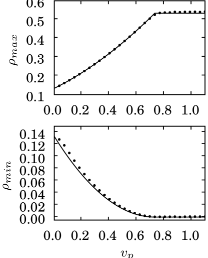
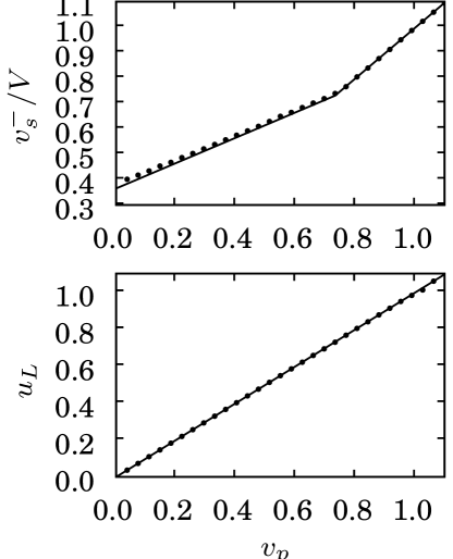
Figure 3: Comparisons of the analytical theory (solid curves) and numerical simulations (dots) for different DSW parameters as functions of the piston velocity $v_{p}$. LEFT: $\rho_{max}$ (top) and $\rho_{min}$ (bottom). Maximum absolute error in $\rho_{max}$ from eqs. (8) and (14) is 0.0088. Maximum absolute error in $\rho_{min}$ from eq. (11) is 0.010. RIGHT: Top depicts the speed of the trailing edge of the piston DSW for $v_{p}<2\sqrt{\rho_{R}}=0.73$ and TW velocity $V$ of locally periodic wave for $v_{p}\geq 2\sqrt{\rho_{R}}$. Bottom shows the validity of the boundary condition (4). Maximum absolute error in $v_{s}^{-}/V$ from eqs. (10) and (13) is 0.018. Maximum absolute error in $u_{L}$ from eq. (4) is 0.013.

The analogous piston viscous shock wave problem in shallow water is discussed in, e.g. Courant and Friedrichs (1948); the 1d equations are equivalent to eqs. (2) when $\varepsilon=0$, $V\equiv 0$ and a dissipative regularization is used whenever a shock forms. The asymptotic solution is found by assuming a simple wave and incorporating the boundary condition (4). In this case, one finds that the shock speed ($v_{s}$) is always larger than the piston speed ($v_{p}$), i.e. one finds $v_{s}-v_{p}=v_{p}\rho_{R}/(\rho_{L}-\rho_{R})>0$.

The analysis in this work shows that techniques from VSW theory, simple wave solutions and suitable jump conditions, are useful in the study of DSWs. Nevertheless, DSWs can lead to very different phenomena.