The CO Molecular Outflows of IRAS 16293–2422 Probed by the Submillimeter Array

Abstract

We have mapped the proto-binary source IRAS 16293–2422 in CO 2–1, ¹³CO 2–1, and CO 3–2 with the Submillimeter Array (SMA). The maps with resolution of 1$\farcs$5–5″ reveal a single small scale ($\sim$3000 AU) bipolar molecular outflow along the east-west direction. We found that the blueshifted emission of this small scale outflow mainly extends to the east and the redshifted emission to the west from the position of IRAS 16293A. A comparison with the morphology of the large scale outflows previously observed by single-dish telescopes at millimeter wavelengths suggests that the small scale outflow may be the inner part of the large scale ($\sim$15000 AU) E–W outflow. On the other hand, there is no clear counterpart of the large scale NE–SW outflow in our SMA maps. Comparing analytical models to the data suggests that the morphology and kinematics of the small scale outflow can be explained by a wide-angle wind with an inclination angle of $\sim$30°–40° with respect to the plane of the sky. The high resolution CO maps show that there are two compact, bright spots in the blueshifted velocity range. An LVG analysis shows that the one located 1″ to the east of source A is extremely dense, n(H₂) $\sim$10⁷ cm^-3, and warm, T${}_{\rm kin}>$ 55 K. The other one located 1″ southeast of source B has a higher temperature of T${}_{\rm kin}>$ 65 K but slightly lower density of n(H₂) $\sim$10⁶ cm^-3. It is likely that these bright spots are associated with the hot core-like emission observed toward IRAS 16293. Since both two bright spots are blueshifted from the systemic velocity and are offset from the protostellar positions, they are likely formed by shocks.

1 Introduction

Outflow phenomena have been recognized as an important phase in the star formation processes. It is generally accepted that when stars are formed by gravitational infall, outflows transfer excess angular momentum out of the system (e.g., Shu, Adams, & Lizano, 1987). Outflows are observed at various wavelengths from the radio to the ultraviolet, among which the millimeter/submillimeter bands probe the molecular outflows. Molecular outflows, recognized as high-velocity wings in CO and other molecular lines, are considered to be the ambient gas entrained or pushed by protostellar winds. By observing molecular outflows, we can determine their physical, kinematic and chemical properties, trace the mass-loss history of protostars, and probe the early phases of the star formation process (Arce et al. 2007, and references therein).

IRAS 16293–2422 (hereafter referred to as I16293) is a well-studied proto-binary system located in the nearby molecular cloud complex L 1689. The distance to L 1689 is often assumed to be 160 pc (Whittet, 1974), however some recent studies suggested a distance of $\sim$120 pc (de Geus et al., 1989; Knude & H$\o$g, 1998). In this paper we adopt 120 pc as the distance. The projected separation of the two protostars is $\sim$5″ (Mundy et al., 1992), which then corresponds to 600 AU. I16293 is classified as a Class 0 young stellar object (YSO) since this system is undetectable at wavelengths shorter than 10 $\mu$m and shows a spectral energy distribution (SED) with very low temperature (André & Monterle, 1994). The bolometric luminosity of I16293 is estimated to be $\sim$36 $L_{\odot}$ (Correia, Griffin, & Saraceno, 2004). I16293 is known to have a quadrupolar outflow (Walker et al., 1988; Mizuno et al., 1990); one bipolar pair extends along the east (blue) and west (red) (hereafter the E–W pair) directions, while the other one has an orientation from northeast (red) to southwest (blue) (hereafter the NE–SW pair) with an inclination angle of 30^∘–45^∘ (Hirano et al., 2001) or 65^∘ (Stark et al., 2004). The NE–SW pair is more collimated, and its axis crosses the position close to the SE continuum source IRAS 16293A (hereafter source A). Therefore this pair has been thought to be powered by source A (e.g., Walker et al., 1988; Mundy, Wootten, & Wilking, 1990). On the other hand, the E–W pair is not as well collimated and its axis, though not well defined, seems to pass to the north of source A, where the continuum source IRAS 16293B (hereafter source B) is the only possible driving YSO. Hence source B has often been assumed as the driving source of the E–W pair. Stark et al. (2004) showed that source B has very narrow line widths, a low luminosity, and is not evidently associated with high-velocity gas. They interpreted source B as a T–Tauri star that drove the E–W pair and that the E–W pair is now a fossil flow. However, these interpretations are based on observations at low angular resolution (i.e., $>$5″), that are insufficient to resolve the two protostars and reveal the relation between the quadrupolar outflow and the binary.

In fact, using higher angular resolution observations Chandler et al. (2005) proposed an alternative interpretation. They resolved source A into four components, two at 1 mm and another two at 7 mm, and suggested that two of them are responsible for driving the NE–SW and the E–W pair, respectively. In addition, Chandler et al. (2005) proposed that source B is actually much younger than previously interpreted and may have not yet begun the phase of mass loss. Their proposition was, however, made based on (1) the dust continuum morphology and proper motions of source A, and (2) the velocity structures of emission of H₂CO, H₂S, and SO, rather than CO, which is a much better tracer of the overall outflow structure free from chemical peculiarities and shocks.

In order to study the molecular outflows in the vicinity of I16293 in more detail, we have carried out CO 2–1, ¹³CO 2–1, and CO 3–2 observations at higher angular resolutions using the Submillimeter Array (SMA). Our SMA observations provide sufficient angular and spectral resolution in the CO lines to resolve the kinematics and the structure of the outflow in the central region of I16293. In this paper, we summarize the observational details in §2; present our SMA CO 2–1, ¹³CO 2–1, and CO 3–2 results in §3; discuss the outflow driving mechanism, physical parameters of the outflow, and the kinematics in the vicinity of I16293 in §4.

2 Observations

The Submillimeter Array (SMA) (Ho, Moran, & Lo, 2004) observations of the CO J=2–1 (230.538 GHz), CO 3–2 (345.796 GHz), and ¹³CO 2–1 (220.399 GHz) transitions were carried out during February 2003 to February 2005. The phase tracking center was $\alpha$(J2000) = 16^h32^m22.91^s, $\delta$(J2000) = $-$24^∘28^′35.52″. The bandwidth of the spectral correlator was 656 MHz in 2003 and 2 GHz in 2005. The frequency resolution used was 812.5 kHz, corresponding to the velocity resolution of 1.06 km s^-1 at 230 GHz and 0.70 km s^-1 at 345 GHz. The field of view of the array is $\sim$54″ at 230 GHz and $\sim$36″ at 345 GHz. The CO 2–1 and ¹³CO 2–1 lines were observed simultaneously on 18 February 2005 with 6 antennas, providing 15 baselines ranging from 10 to 70 m. The CO 3–2 data were observed on February 26 and April 23 in 2003 with 4 and 5 antennas, respectively, providing 10 independent baselines ranging from 12 to 120 m. We note that the CO 3–2 observations provide fewer short baselines than the CO 2–1 observations, therefore the CO 3–2 data are less sensitive to extended structures.

The visibility data were calibrated using the MIR software package originally developed for Owens Valley Radio Observatory (Scoville et al., 1993; Qi, 2005) and modified for the SMA. The absolute flux calibration and bandpass calibration were done by observing Callisto (on 2003 February 26), Ganymede (on 2003 April 23), and Uranus (on 2005 February 18). The uncertainty in the absolute flux scale is estimated to be $\sim$10%. The visibility phase and amplitude calibration was achieved by observing the quasars NRAO 530 (J1733-130) in 2003 and J1743–038 in 2005. The continuum level was measured from line-free channels in the calibrated visibility data. The MIRIAD and the NRAO AIPS packages were used to make the spectral images and for further analysis. The maps were restored using uniform weighting, resulting in synthesized beam sizes of 4$\farcs$7$\times$2$\farcs$5 with a position angle of 0.0^∘ for the CO 2–1, 4$\farcs$9$\times$2$\farcs$6 with a position angle of 1.5^∘ for the ¹³CO 2–1, and 1$\farcs$6$\times$1$\farcs$4 with a position angle of 26.2^∘ for the CO 3–2. The rms noise levels of the channel maps with $\sim$1 km s^-1 width are $\sim$0.15 Jy beam^-1 for the CO 2–1, $\sim$0.13 Jy beam^-1 for the ¹³CO 2–1, and $\sim$0.3 Jy beam^-1 for the CO 3–2.

3 Results

3.1 CO 2–1

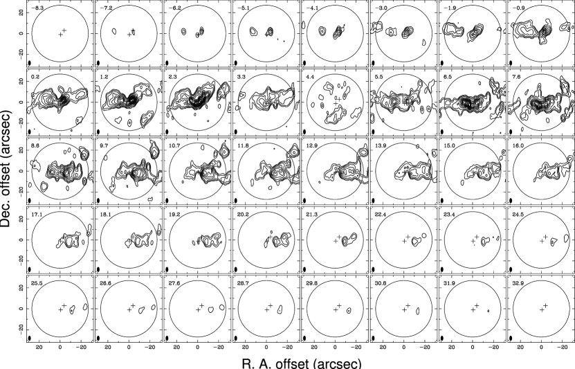
Figure 1: Velocity channel maps of the CO 2–1 emission. Offsets (in arcseconds) are with respect to the phase tracking center, $\alpha=$ 16^h32^m22.91^s and $\delta=$ $-$24^∘28^′35.52″(J2000). The contour levels correspond to $-$5$\sigma$, 5$\sigma$, 10$\sigma$, 20$\sigma$, then increase in every 20$\sigma$ step. The 1$\sigma$ level is 0.15 Jy beam^-1. The crosses indicate the positions of the continuum sources A and B; the open circle is the SMA field of view at 230 GHz, and the filled ellipse indicates the synthesized beam. Note that the primary beam correction is not applied to the data.

Fig. 1 shows the velocity channel maps of the CO 2–1 emission uncorrected for the primary beam attenuation. The CO 2–1 emission is shown in the channels from $V_{\rm LSR}$ = $-$7.2 km s^-1 to 31.9 km s^-1. In most of the channels, the spatial distribution of the CO 2–1 emission is elongated along the east-west direction. It is likely that this elongated CO emission originates from the molecular outflow previously imaged on larger scales (Stark et al., 2004). The CO emission at $V_{\rm LSR}$ = 4.4 km s^-1 is scattered over the field of view. Since this velocity channel is close to the cloud systemic velocity of $V_{\rm LSR}$ = 4.0 km s^-1 (Mizuno et al., 1990), most of the emission has been resolved out due to the lack of short baselines. The CO distribution at $V_{\rm LSR}$ = 3.3 km s^-1 and $V_{\rm LSR}$ = 5.5 km s^-1 shows the east-west elongation, suggesting that the CO emission at these channels comes from the outflowing gas even though the velocity offset from the systemic velocity is small. Therefore, we infer that the CO 2–1 emission seen in the channels from $V_{\rm LSR}$ = $-$7.2 km s^-1 to 3.3 km s^-1 is the blueshifted outflow component and that in the channels from $V_{\rm LSR}$ = 5.5 km s^-1 to 31.9 km s^-1 is the redshifted outflow component.

The blueshifted emission is extended to the east of source A and the west of source B as well. The eastern component is seen in most of the blueshifted channels from $V_{\rm LSR}$ = $-$7.2 km s^-1 to 3.3 km s^-1, while the western component is in the velocity range from $V_{\rm LSR}$ = $-$0.9 km s^-1 to 3.3 km s^-1, and is closer to the systemic velocity compared to the eastern component. As shown in the velocity channels from $V_{\rm LSR}$ = $-$0.9 km s^-1 to 1.2 km s^-1, the eastern blueshifted component has a fan shape pointing to source A with a position angle of $\sim$75^∘.

The redshifted emission extends to the east and the west of source A. The eastern redshifted component mostly overlaps with the eastern blue emission. The western redshifted component has a fan shape structure with its apex at the position of source A at P.A. $\sim$90^∘. This structure appears from $V_{\rm LSR}$ = 8.6 km s^-1, and the emission moves away from the source as the velocity increases.

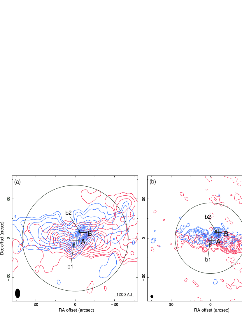
Figure 2: a: Integrated blueshifted (blue contours) and redshifted (red contours) CO 2–1 maps. The emission is integrated over the velocity channels from $V_{\rm LSR}=-$7.2 km s^-1 to 3.3 km s^-1 on the blueshifted side and from $V_{\rm LSR}=$ 5.5 km s^-1 to 31.9 km s^-1 on the redshifted side. Contours are drawn at $-$5$\sigma$, 5$\sigma$, 10$\sigma$, 20$\sigma$, then every 20$\sigma$ step. The 1$\sigma$ levels are 0.6 Jy beam^-1 km s^-1 for the blueshifted component and 0.9 Jy beam^-1 km s^-1 for the redshifted component. The two crosses denote the positions of the two continuum sources. Positions of the two prominent compact components are labeled (b1 and b2). The open circle indicates the field of view at 230 GHz, and the filled ellipse indicates the synthesized beam size. b: Same as Fig. 2a for the CO 3–2. The emission is integrated over the velocity channels from $V_{\rm LSR}=-$7.5 km s^-1 to 3.5 km s^-1 on the blueshifted side, and from $V_{\rm LSR}=$5.5 km s^-1 to 31.5 km s^-1 on the redshifted side. Contour levels are 3$\sigma$, 5$\sigma$, and every 5$\sigma$ steps. The 1$\sigma$ levels are 1.4 Jy beam^-1 km s^-1 for the blueshifted component and 2.3 Jy beam^-1 km s^-1 for the redshifted component. The open circle is the field of view at 345 GHz, and the solid oval indicates the synthesized beam size. Note that the primary beam correction is not applied to the data.

The total integrated intensity (zeroth moment) maps of the blueshifted and redshifted CO 2–1 line emission are presented in Fig. 2a (uncorrected for primary beam attenuation). In the blueshifted component, there are two prominent peaks 1″ to the east of source A (labeled b1) and 1″ southeast of source B (labeled b2). The peak brightness temperature of CO 2–1 emission at b1 and b2 are 57 K and 63 K, respectively. These two peaks are seen in all the blueshifted channels (Fig. 1) starting from $V_{\rm LSR}$ = $-$6.2 km s^-1. We note that both b1 and b2 have not been resolved in the previous CO outflow maps observed with the single-dish telescopes (Stark et al., 2004).

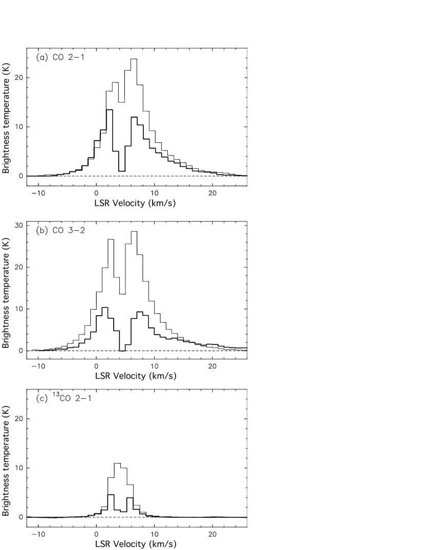
Figure 3: A comparison of the CO 2–1 (a), CO 3–2 (b) and ¹³CO 2–1 (c) spectra observed with the SMA (black histograms) and the JCMT (grey histograms) at the pointing center. The SMA data were first primary beam corrected, and the spectra were smoothed to have the same angular resolution as the JCMT data, i.e., 14″ for the CO 3–2 and 21″ for the CO and ¹³CO 2–1. The JCMT spectra are resampled to have the same velocity resolution as that of the SMA data and converted into brightness temperature by assuming the main beam efficienciies, ${\eta}_{\rm MB}$, to be 0.69 for the CO 2–1 and ¹³CO 2–1, and 0.63 for the CO 3–2.

In Fig. 3a we compare the CO 2–1 spectrum observed by the SMA with that observed by the JCMT. We have applied the primary beam correction, smoothed the SMA map to have a 21″ Gaussian beam, which is same as the JCMT beam at 230 GHz, and obtained the spectrum at the phase tracking center. The JCMT spectrum was resampled to have the same velocity resolution as the SMA data. To convert the antenna temperature $T_{\rm A}$* into brightness temperature, we adopted a main beam efficiency, ${\eta}_{\rm MB}$, of 0.69 for the JCMT at 230 GHz. It is shown that the SMA recovered most of the flux in the velocity range lower than $V_{\rm LSR}\sim$2 km s^-1, indicating that most of the blueshifted emission in this velocity range comes from the compact regions labeled b1 and b2. The SMA spectrum is slightly brighter than the JCMT spectrum in several channels, probably due to the calibration uncertainties in both the SMA and JCMT data. In the redshifted velocity range, the SMA recovered $\sim$70% of the flux at $V_{\rm LSR}>10$ km s^-1. The flux in the velocity range close to the systemic velocity is recovered $\sim$60% except the channel of the deep absorption dip at $V_{\rm LSR}=$ 4.4 km s^-1. At this velocity, absorption caused by the foreground cloud also contributes to the total absence of emission in the interferometric map because the JCMT spectrum also shows a deep absorption dip at the same velocity.

3.2 CO 3–2

The CO 3–2 total integrated intensity (zeroth moment) map is shown in Fig. 2b (uncorrected for primary beam attenuation). The emission is integrated over the velocity channels from $V_{\rm LSR}=$ $-$7.5 km s^-1 to 3.5 km s^-1 on the blueshifted side, and from $V_{\rm LSR}=$ 5.5 km s^-1 to 31.5 km s^-1 on the redshifted side. There is no significant emission in the velocity channel centered at $V_{\rm LSR}=$ 4.5 km s^-1. The CO 3–2 emission in this velocity range arises from the extended ambient cloud and is poorly sampled by the uv coverage of the CO 3–2 data. There are two bright blueshifted components, one located 2″ southeast of source A and the other located 1″ southeast of source B, that are likely to be the counterparts of b1 and b2 identified in the CO 2–1 map (see Fig. 2a). The peak brightness temperature of CO 3–2 emission is 39 K at b1 and 55 K at b2. These two components are connected by faint emission. The blueshifted emission extending toward the northeast with a P.A. of $\sim$70^∘ corresponds to the eastern blueshifted emission in the CO 2–1 map. As in the case of CO 2–1, the redshifted emission extends to the east and west of source A.

In order to estimate the missing flux, we have smoothed the SMA CO 3–2 map to 14″ resolution, which is the HPBW of the JCMT at 345 GHz, and compared the spectrum at the phase tracking center with that obtained by the JCMT (Fig. 3b). The primary beam correction was applied to the SMA CO 3–2 map before it was smoothed. The JCMT spectrum was converted into the brightness temperature unit by assuming ${\eta}_{\rm MB}=0.63$ at 345 GHz. Fig. 3b shows that the missing flux of the SMA CO 3–2 data is larger than that of the CO 2–1 except for the high-velocity part of the redshifted wing at $V_{\rm LSR}~{}\gtrsim$ 14 km s^-1, where most of the flux is recovered by the SMA. The SMA recovered $\sim$50% of the CO 3–2 flux in the velocity ranges $-$9.0 $<V_{\rm LSR}<$ 2.0 km s^-1 and 6.0 $<V_{\rm LSR}<$ 13.0 km s^-1. That more missing flux is evident in the CO 3–2 data than the CO 2–1 data is likely due to it containing fewer short baselines, as mentioned in §2.

3.3 ¹³CO 2–1

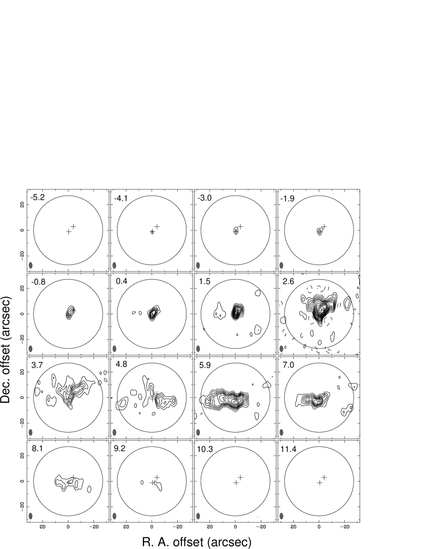
Figure 4: Velocity channel maps of the ¹³CO 2–1 emission. The contours start at $-$5$\sigma$ and are drawn every 5$\sigma$ step until 30$\sigma$, and every 10$\sigma$ in the range above 30$\sigma$. The 1$\sigma$ level is 0.13 Jy beam^-1. The crosses indicate the positions of the continuum sources A and B; the open circle is the SMA field of view at 230 GHz. Note that the primary beam correction is not applied to the data.

Fig. 3c compares the ¹³CO spectrum observed with the SMA and that observed with the JCMT. The SMA spectrum was obtained after we corrected for the primary beam attenuation and smoothed to 21″ resolution. Due to a software problem, the velocity values of the ¹³CO 2–1 data were not recorded correctly. We found that the ¹³CO 2–1 spectrum observed with the SMA was blueshifted by $\sim$1 km s^-1 with respect to that observed with the JCMT. Therefore, we calibrated the velocity of each channel in the SMA data using the ¹³CO 2–1 spectrum observed with the JCMT. Most of the ¹³CO 2–1 flux is recovered by the SMA at $V_{\rm LSR}<$ 2.0 km s^-1. The velocity channel maps of the ¹³CO 2–1 emission presented in Fig. 4 (uncorrected for primary beam attenuation) show that emission in this velocity range mainly comes from the compact source close to source A. It is likely that this component corresponds to b1 in the CO 2–1 map. On the other hand, the brightest component b2 in the CO 2–1 map is less significant in the ¹³CO 2–1. It is identified as a northwestern extension of the emission in the velocity channels from $-$0.8 to 1.5 km s^-1. The ¹³CO emission extends to the east of source A in the redshifted velocity channels at $V_{\rm LSR}$ = 5.9 km s^-1 and 7.0 km s^-1, and extends to the east and west of source A at $V_{\rm LSR}$ = 8.1 km s^-1. It should be noted that a similar structure is seen in the velocity channel maps of the CO 2–1 (see Fig. 1), suggesting that the ¹³CO 2–1 emission in this velocity range arises from the dense part of the outflow. The ¹³CO 2–1 flux recovered by the SMA is 60–70% in the velocity channels from $V_{\rm LSR}$ = 5.9 km s^-1 to 9.2 km s^-1. In the velocity channels at $V_{\rm LSR}$ = 2.6 km s^-1 and 3.7 km s^-1, the ¹³CO 2–1 map shows a V-shaped structure. Since the southwestern and southeastern edges of the ¹³CO 2–1 correspond to the northern edges of the western and eastern lobes, respectively, it is likely that the ¹³CO 2–1 emission in this velocity range comes from the envelope excavated by the outflow. Note that the primary beam correction is not applied to the images shown in Fig. 4.

4 Discussion

4.1 Outflows in the vicinity of IRAS 16293–2422

4.1.1 Driving source

As was shown in §3, the CO 2–1 and 3–2 maps observed with the SMA clearly show small scale outflow emission in the vicinity of I16293. It is quite natural to assume that the CO 2–1 and 3–2 outflow emission has the same origin. Each of the CO 2–1 and 3–2 outflows has a blueshifted component extending to the east and a redshifted component extending to the west of source A (see Fig. 2a and 2b). In the CO 2–1 channel maps, both the eastern blueshifted component and the western redshifted component show fan-shaped patterns with their apexes pointing toward source A. Although the eastern redshifted component is less clearly extending from the position of source A, its coincidence with the eastern blueshifted emission suggests that the eastern blue- and redshifted components represent the front side and the back side of a single outflow lobe, respectively. Such an outflow lobe showing both blue- and redshifted emissions together is likely to be an outflow with a wide opening angle and an axis close to the plane of the sky (Cabrit & Bertout, 1986). These morphological characteristics of the small scale outflow suggest that it is most likely driven by source A.

The direction of the outflow axis is rather difficult to define clearly. The western redshifted lobe in CO 2–1 shows a position angle of almost $-$90^∘, while the blue- and redshifted eastern lobes show position angles of $\sim$75^∘. The axis of the CO 3–2 outflow is approximately along a position angle of 80^∘. These results suggest that the axis of the small scale outflow is approximately the east-west direction. The difference in direction between the blue- and redshifted components of the CO 2–1 emission, and the CO 2–1 and 3–2 emission, could also indicate that the high velocity gas comprises emission from two or more outflows. There may be an interaction between the wind or jet driving the large scale NE–SW outflow and the molecular gas, as indicated by the offset of shock-tracing molecule line emission peaks to the NE of source A (Chandler et al. 2005). However, the bulk of the CO emission we observe is consistent with a predominantly E–W outflow.

4.1.2 Comparisons with the large scale outflows

It is important to know the relationship between the small scale ($\sim$3000 AU) outflow observed with the SMA and the large scale ($\sim$15000 AU) outflows previously observed with single-dish telescopes even though the size scales are quite different between them. We should note that the missing flux and the single field of view in the SMA observations prevent us from directly relating the two types of outflows on these very different scales. Nevertheless, morphological comparisons of the small and large scale outflows could allow us to infer their relationship.

Single-dish observations showed two large scale outflows; one is the E–W pair and the other is the NE–SW pair (Walker et al., 1988; Mizuno et al., 1990; Lis et al., 2002; Stark et al., 2004). The blue- and redshifted lobes of the E–W pair are located to the east and the west, respectively, showing the same velocity trend as the small scale outflow. The outflow axes of these two outflows are also similar. These facts naturally suggest that the small scale outflow is the inner part of the large scale E–W pair, and that the bulk of the CO emission observed by the SMA is due to the E–W outflow. If this is the case, then the E–W pair is not a fossil flow but a currently active one, and the driving source of the E–W pair is most likely to be source A.

Do the SMA maps show any counterparts of the NE–SW pair? Chandler et al. (2005) proposed that the driving source of the NE–SW pair is one of the radio sources, A2, based on its bipolar morphology along the NE–SW direction in their 43 GHz map. However, our SMA maps show no counterpart of the NE–SW pair, if we consider the small scale outflow mapped with the SMA as the inner part of the E–W pair. One possible reason for why there is no counterpart of the NE–SW pair in the SMA maps is that the NE–SW outflow lobes are located outside the SMA field of view at both 230 and 345 GHz. In fact, single-dish maps (Mizuno et al., 1990; Lis et al., 2002; Stark et al., 2004) show that both blue- and redshifted lobes are detached by $\sim$1′ from the centroid of I16293. This implies that the NE–SW pair is older than the E–W pair, so the NE–SW pair has already cleaned out the gas along its travel direction. However this interpretation is totally different from those of previous studies, where the NE–SW pair is considered younger than the E–W pair. On the other hand, the NE–SW pair is better collimated than the E–W pair. Observations of CO outflows of YSOs at different evolutionary stages suggest that the opening angle of the outflow lobe becomes larger as the central source evolves (e.g., Arce & Sargent, 2006). If we take this into account, it is natural to consider that the well-collimated NE–SW pair is younger than the E–W pair. It is possible that the small scale counterpart of the NE–SW pair is absent because this outflow is currently inactive due to its episodic nature. Eposodic outflows have been found in several YSOs, such as L1157 (e.g., Gueth et al., 1996). Since there is no counterpart of the NE–SW pair in our SMA maps, we are unable to determine if the NE–SW outflow is driven by source A of B, and to support or refute the different claims by previous studies regarding this flow (Stark et al., 2004; Chandler et al., 2005).

4.2 Kinematics of the small scale outflow

Many models have been proposed to explain the relation between molecular outflows and protostellar jets. Of these, two scenarios are considered plausible: (1) the jet-driven model, where molecular outflows consist of ambient gas swept up by the bow shock of the jet head (Raga & Cabrit, 1993; Masson & Chernin, 1992; Chernin et al., 1994), and (2) the wind-driven model, where molecular outflows are the swept-up gas entrained by wide-angle magnetized wind (Shu et al., 1991, 2000; Li & Shu, 1996). These scenarios have different kinematical features in a Position–Velocity (P–V) diagram obtained from a cut along the outflow axis. The jet-driven model will produce a convex structure in such a P–V diagram with high velocity components at the jet head; while the wind-driven model will introduce a parabolic structure that originates from the central star (e.g., Lee et al., 2000).

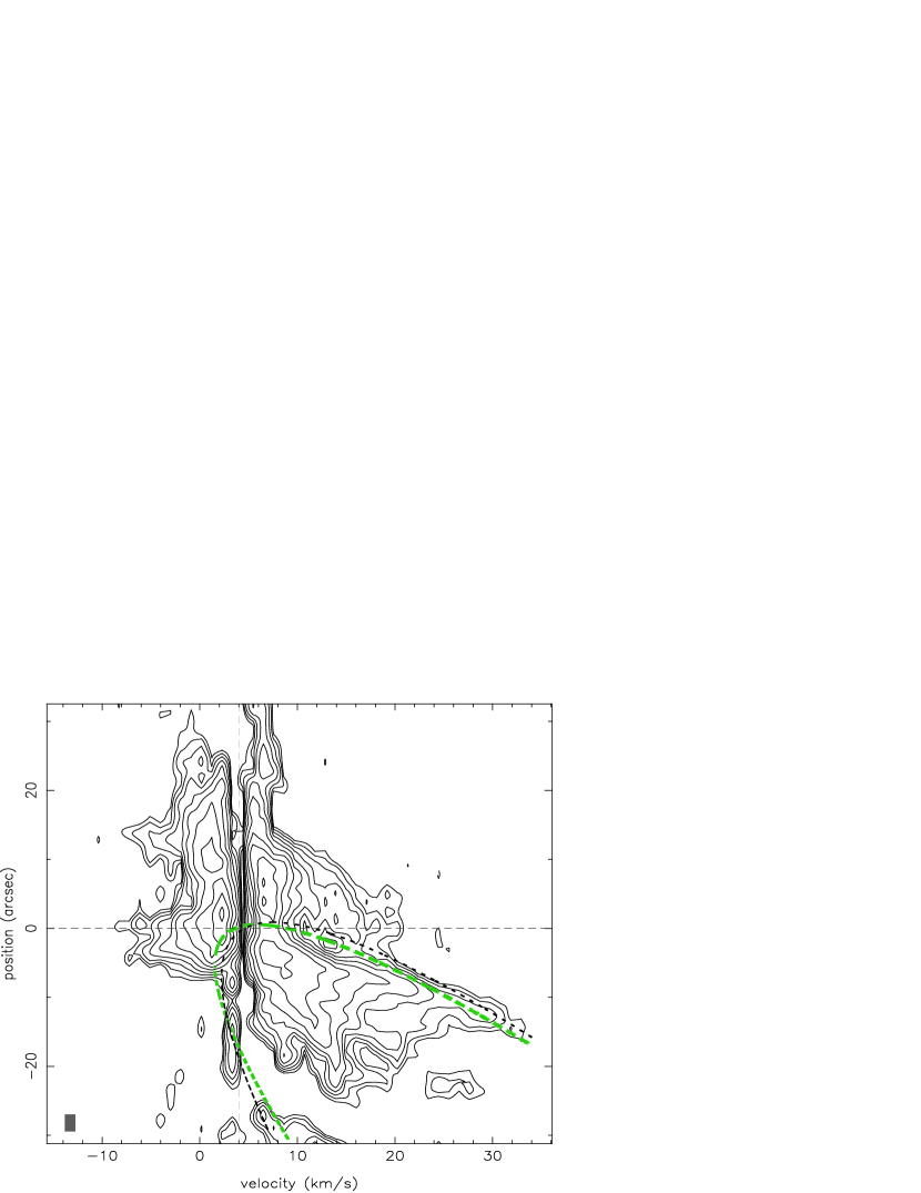
Figure 5: Position-velocity (P–V) diagram of the CO 2–1 along a cut at P.A. = 90^∘ through the position of source A. Contours are logarithmic at: 0.90, 1.43, 2.26, 3.58, 5.68, 9.00, 14.3, 22.6, and 35.8 K. The horizontal thin dashed line is the position of source A; while the vertical thin dashed line labels the systemic velocity V_sys=4.0 km s^-1. The green curve: wide-angle wind model curve produced by i=30^∘, $C$=0.20 arcsec^-1, and v₀=1.30 km s^-1 arcsec^-1. The black curve: wide-angle wind model curve produced by i=40^∘, $C$=0.10 arcsec^-1, and v₀=0.80 km s^-1 arcsec^-1. The filled square at the bottom left denotes the spacial and velocity resolution.

In a CO 2–1 P–V diagram, extracted along the outflow axis at P.A. = 90^∘ (Fig. 5), we found that the western redshifted lobe shows a parabolic shape, as is expected from the wind-driven model. We therefore adopted the simplified analytical model of a wind-driven shell proposed by Lee et al. (2000) to study the kinematics of the small scale outflow. In the cylindrical coordinate system, the structure and velocity of the shell can be written as follows:

$$z=CR^{2},{\it v}_{R}={\it v}_{0}R,{\it v}_{z}={\it v}_{0}z,$$ (1)

where $z$ is the distance along the outflow axis; $R$ is the radial size of the outflow perpendicular to $z$ ; $C$ and $v_{0}$ are free parameters that describe the spatial and velocity distributions of the outflow shell, respectively.

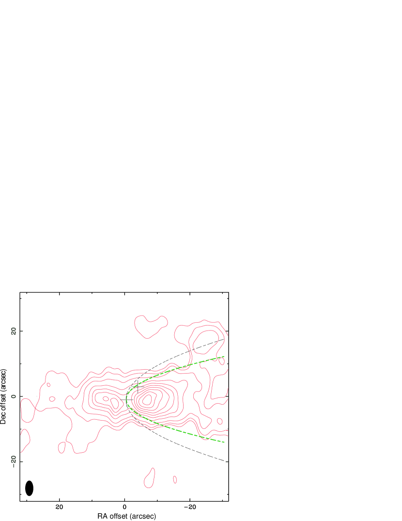
Figure 6: Outflow shell model curves overlaid onto the redshifted CO 2–1 emission. The green line and the black line delineate the curves with $C$ = 0.20 arcsec^-1 and $C$ = 0.10 arcsec^-1, respectively. Both curves were produced by assuming the inclination angle of the axis from the plane of the sky to be 30^∘.

First, we generated the model curve that delineates the outflow shell feature (see Fig. 6), to determine the free parameter $C$. In Fig. 6 the green line and the black line delineate the curves produced by $C=$ 0.20 arcsec^-1 and $C=$ 0.10 arcsec^-1, respectively. Both curves assume the inclination angle of the axis from the plane of the sky, i to be 30^∘. However, the curve is insensitive to the inclination angle if i is smaller than 40^∘. Since both eastern and western lobes have opening angles of 60^∘–80^∘, and are accompanied by the CO emission component with opposite velocity shifts (i.e. the eastern blue lobe is accompanied by the redshifted component and the western red lobe by the blueshifted component), it is unlikely that the inclination angle is larger than 40^∘. Next, we determined v₀ and i by comparing the velocity pattern of the model curve with the observed P-V diagram. The green curve in Fig. 5 was produced by i = 30^∘, $C=$ 0.20 arcsec^-1, and v₀ = 1.3 km s^-1 arcsec^-1; while the dashed curve was produced by i = 40^∘, $C=$ 0.10 arcsec^-1, and v₀ = 0.8 km s^-1 arcsec^-1. A wind-driven outflow model predicts the “Hubble law” velocity structure, that is the velocity increases as the emission moves away from the central source (e.g., Shu et al., 1991; Lee et al., 2000). As we have mentioned in §3.1, the redshifted lobe of the small scale outflow has this signature. Hence, our simple modeling qualitatively indicates that the driving mechanism for the small scale outflow could be a wide-angle wind inclined to the plane of the sky by $\sim$30^∘ to 40^∘. The dynamical age of the small scale outflow is given by 1/v₀ and is 450–700 years.

It should be noted that the wind-driven model does not contradict to the evidence of a precessing jet presented by Chandler et al. (2005). Recent numerical simulations of magnetocentrifugal winds predict an on-axis density enhancement within the $X$-wind type of wide opening angle wind (Li & Shu, 1996; Shang et al., 2002, 2006), and so it is possible to have a jet-like feature in such a model that does not show up in CO observations.

4.3 Physical parameters of the small scale outflow

We estimated the outflow mass using the CO 2–1 and ¹³CO 2–1 data cubes corrected for the primary beam attenuation and assuming LTE conditions. Since the peak brightness temperature of the CO emission reaches $\sim$50 K, we assumed 50 K as an excitation temperature. We adopted an H₂ to CO abundance ratio of 10⁴ and a mean atomic weight of the gas of 1.36. A comparison between the channel maps of CO 2–1 (Fig. 1) and those of ¹³CO 2–1 (Fig. 4) suggests that the CO 2–1 emission is significantly optically thick in the low-velocity redshifted component at $V_{\rm LSR}\sim$5–9 km s^-1 and the low-velocity blueshifted component at $V_{\rm LSR}\sim$0–2 km s^-1. The ¹³CO 2–1 emission is also detected in the positions of the bright spots b1 and b2; however, we excluded these components from our calculation. The physical conditions of these bright spots are discussed in the next subsection. At velocities where the ¹³CO emission is detectable, we estimated the optical depth of the CO 2–1 line using the following equation:

$$\frac{S_{\nu}(\rm{CO})}{S_{\nu}(^{13}\rm{CO})}=\frac{[\rm{CO}]}{[^{13}\rm{CO}]}\left(\frac{1-e^{-\tau}}{\tau}\right),$$ (2)

where [CO]/[¹³CO] is the abundance ratio between CO and ¹³CO that is assumed to be 77 (Wilson & Rood, 1994). The optical depth of the CO 2–1 emission in the low-velocity redshifted component is estimated to be $\sim$3–36 in the western lobe and $\sim$6–24 in the eastern lobe, and that of the low-velocity blueshifted component is $\sim$2–17 in the eastern lobe. Outflow masses in the optically thick velocity channels were corrected using:

$$M_{thick}=\sum m(v_{i})=m^{\prime}(v_{i})\left(\frac{\tau_{i}}{1-e^{-\tau(v_{i})}}\right),$$ (3)

where m^′(v_i) is the mass at velocity v_i without optical depth correction; m($v_{i}$) is the mass after optical depth correction; $\tau_{i}$ represents the optical depth of CO 2–1 at velocity v_i. Outside the velocity ranges where the ¹³CO emission was observed, we assumed that the CO emission is optically thin, and obtained the mass by $M_{thin}=\sum m^{\prime}(v_{i})$. The total mass of the outflow was obtained by $M_{total}=M_{thin}+M_{thick}$. Table 1 summarizes the masses of the blueshifted and redshifted components in the eastern and western lobes. The optically thick part of the spectrum dominates the outflow mass calculations. The outflow masses are underestimated by an order of magnitude without the correction for optical depth. Since significant flux is missed in the low velocity range due to the lack of short baseline data and absorption by foreground clouds, the masses derived here are lower limits. In both eastern and western lobes, the redshifted component is significantly more massive than the blueshifted component. This suggests that dense ambient gas exists behind the outflow lobes, so that the blueshifted component in the front can expand rather freely, while the redshifted component in the back needs to push more material.

The dynamical parameters of the flow are summarized in Table 2. Table 2 gives two kinds of values; one is corrected for the inclination effect ($i=$ 35^∘) and the other is without this correction (uncorrected). The inclination angle of 35^∘ is chosen based on the kinematical modeling described in the previous section. In order to compare the energies of the small scale outflow with those of the large scale E–W outflow observed with single-dish telescopes, we estimated the momentum supply rate and the stellar mass loss rate. These dynamical quantities can be derived reasonably well even though the map is incomplete (e.g. Bontemps et al., 1996). The momentum supply rate and the mass loss rate of the small scale outflow lobes are estimated to be $\sim$2$\times$10^-4 $M_{\odot}$ km s^-1 yr^-1 and 9.0$\times$10^-7 $M_{\odot}$ yr^-1, respectively. The CO 1–0 single-dish observational result of I16293 (Mizuno et al., 1990) scaled to a distance of 120 pc suggests that the momentum supply rate and the mass loss rate of the large scale E–W outflow are $\sim$1.6$\times$10^-4 $M_{\odot}$ km s^-1 yr^-1 and $\sim$8.0$\times$ 10^-7 $M_{\odot}$ yr^-1 in the eastern lobe, while those of the western lobe are $\sim$1.1$\times$10^-4 $M_{\odot}$ km s^-1 yr^-1 and $\sim$5.6$\times$10^-7 $M_{\odot}$ yr^-1, respectively. Although the parameters we derived from the SMA data are lower limits, it is likely that the small scale outflow has comparable momentum and energy with the large scale E–W outflow. This may imply that the E–W outflow has been fairly constant in time, if the compact outflow is the inner part of the large scale E–W outflow.

4.4 Nature of the bright, compact components

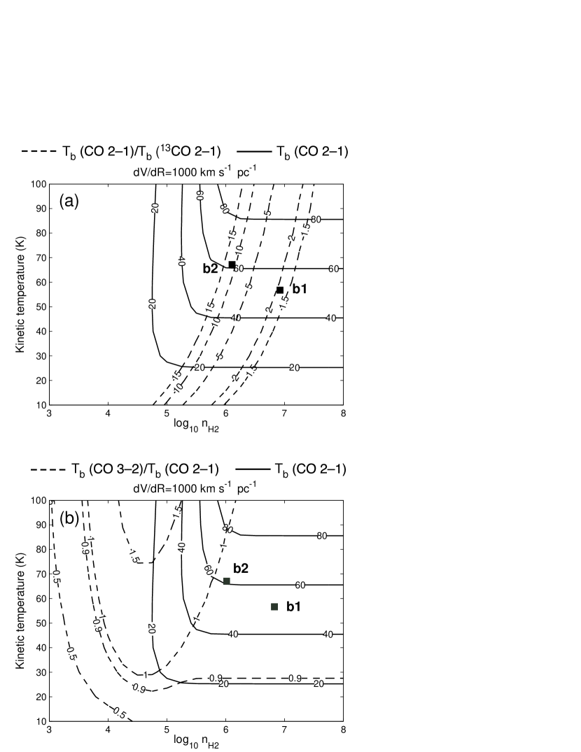
Figure 7: a: Curves of constant line ratios of CO 2–1/¹³CO 2–1 (dashed lines) and constant CO 2–1 intensity (solid lines) as a function of the kinetic temperature and the H₂ number density for $dv/dr$ = 1000 km s^-1 pc^-1. The filled squares denote the corresponding observed values of b1 and b2. b: Curves of constant line ratios of CO 3–2/CO 2–1 (dashed lines) and constant CO 2–1 intensity (solid lines). The locations of b1 and b2 in this diagram correspond to the physical conditions derived from CO 2–1 and ¹³CO 2–1 data.

As shown in §3, the high resolution CO maps reveal two bright and compact components, labeled b1 and b2, at blueshifted velocities (see Fig. 1 and Fig. 2). In order to investigate the nature of b1 and b2, we carried out an LVG calculation (Goldreich & Kwan, 1974; Scoville & Solomon, 1974) using the code developed by Oka et al. (1998). The velocity gradient $dv/dr$ is assumed to be 1000 km s^-1 pc^-1 as estimated from the CO 2–1 line width of $\sim$ 7 km s^-1 and the size of $\sim$0.005 pc of b1 and b2. The LVG calculation result is shown in Fig. 7. Fig. 7a shows the iso-intensity contours of the CO 2–1 line (solid contours) and iso-line ratio contours of CO 2–1/¹³CO 2–1 (dashed contours) as a function of kinetic temperature and H₂ number density. Fig. 7b shows the CO 2–1 iso-intensity contours (solid contours) and iso-line ratio contours of CO 2–1/¹³CO 2–1 (dashed contours).

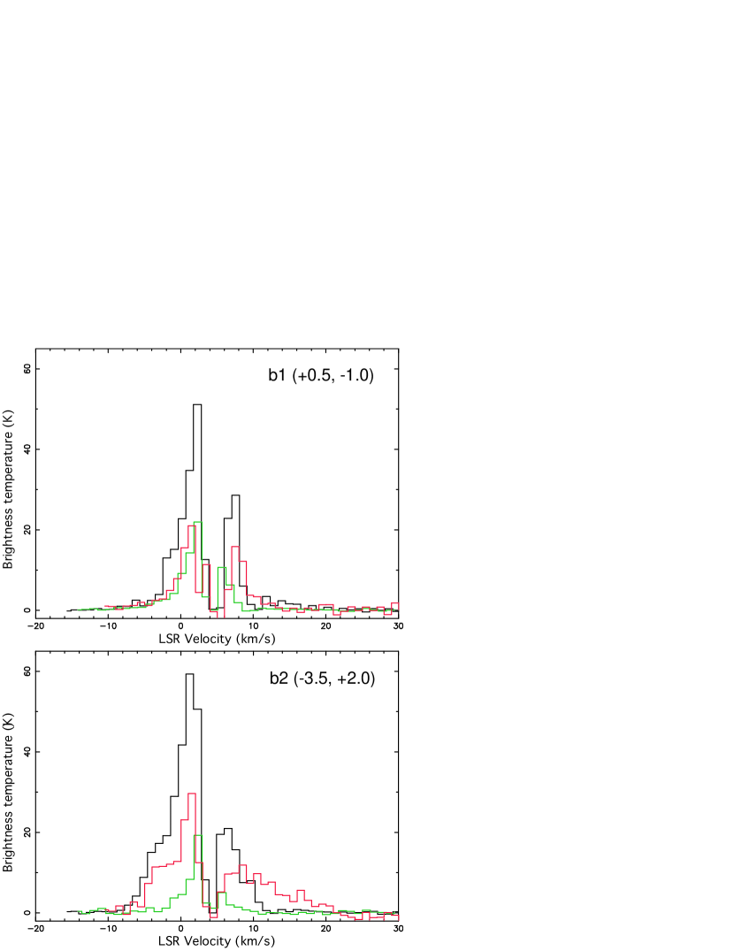
Figure 8: Line profiles of the CO 2–1 (black line), ¹³CO 2–1 (green line) and CO 3–2 (red line) at the compact components b1 and b2. The position offsets of each component with respect to the phase tracking center are labeled in arcseconds at the top right.

In order to compare the CO 3–2, CO 2–1, and ¹³CO 2–1 lines at the positions b1 and b2, we made the maps of these three lines using the visibility data in the range from 10 k$\lambda$ to 52 k$\lambda$, corresponding to the uv range common for the three data sets. The beam sizes in uniform weighting of the CO 3–2, CO 2–1, and ¹³CO 2–1 maps were 3$\farcs$1$\times$2$\farcs$6 (P.A. 5.2^∘), 4$\farcs$7$\times$2$\farcs$5 (P.A. $-$3.0^∘), and 4$\farcs$8$\times$2$\farcs$6 (P.A. 1.5^∘), respectively. In spite of the same uv range limit, the beam size of the CO 3–2 map is different from those of the CO 2–1 and ¹³CO 2–1 due to differet uv coverages. Therefore, we convolved the three maps to the same beam size, i.e. 4$\farcs$9$\times$2$\farcs$7 with a P.A. of 0.0^∘ after the correction of the primary beam attenuation. The CO 3–2, 2–1 and ¹³CO 2–1 spectra obtained at the positions of b1 and b2 are shown in Fig. 8. The brightness temperature of CO 2–1 at the position of b1 is $T_{\rm B}\sim$50 K, and that at b2 is $T_{\rm B}\sim$60 K. The CO 2–1 flux integrated over the velocity range from $V_{\rm LSR}$ = $-$8 km s^-1 to 2 km s^-1 is 102.2 K km s^-1 at b1 and 207.5 K km s^-1 at b2. The ¹³CO 2–1 flux integrated over the same velocity range is 55.9 K km s^-1 at b1 and 18.7 K km s^-1 at b2. Since most of the CO and ¹³CO 2–1 fluxes in this velocity range were recovered by the SMA, the effect of missing flux should not be significant. The CO 2–1/¹³CO 2–1 intensity ratio of 1.8 at b1 suggests that this component is warm ($T_{\rm kin}\sim$55 K) and extremely dense ($n(\rm H_{2})\sim$10⁷ cm^-3). On the other hand, the CO 2–1/¹³CO 2–1 ratio at the position of b2 is $\sim$11, suggesting that b2 is slightly warmer ($T_{\rm kin}\sim$65 K) but less denser ($n(\rm H_{2})\sim$10⁶ cm^-3) than b1.

The CO 3–2 flux integrated over the same velocity range as CO 2–1 is 58.4 K km s^-1 at b1 and 105.6 K km s^-1 at b2. The CO 3–2/2–1 ratio at the positions of b1 and b2 calculated from the integrated intensity values are 0.57 and 0.51, respectively. On the other hand, Fig. 7 shows that the line ratio should be $\gtrsim$0.9 if the CO 2–1 intensity is brighter than 20 K. However, in contrast to CO 2–1, only $\sim$50% of the CO 3–2 flux in this velocity range was recovered by the SMA. If we assume that most of the CO 3–2 flux within the central 14″ region arises from the compact sources b1 and b2, their actual flux values might be twice the calculated values. If we take this effect into account, the CO 3–2/2–1 ratio might be close to 1 at both b1 and b2. Therefore, the CO 3–2 results do not contradict the physical conditions inferred for b1 and b2 from the CO and ¹³CO 2–1 data. We should note that there are two effects that could contribute to a low CO 3–2/2–1 ratio. If the CO emission is assumed to be in LTE and optically thick, the CO 3–2 emission has a higher optical depth than CO 2–1. Therefore if there are temperature gradients due to internal heating sources, the CO 3–2 emission will tend to trace outer and cooler gas. Even for a uniform temperature, the $\tau=$ 1 surface of the CO 3–2 emission with higher optical depth will be more extended and more flux will be resolved out by the interferometer, independent of the other uv coverage issues.

It should also be noted that the kinetic temperature and density derived here are the averaged values over the beam area of 4$\farcs$9$\times$2$\farcs$7. Since the bright spots b1 and b2 are compact, the CO 2–1 brightness temperature at b1 and b2 might be higher if we observe with higher angular resolution. Indeed, the brightness temperatures of CO 2–1 and CO 3–2 at b1 and b2 measured in the higher resolution maps are higher than those of the spectra shown in Fig. 8. Therefore it is possible that the kinetic temperatures at b1 and b2 are higher than those estimated here.

Complex molecules, such as HCOOCH₃ and C₂H₃CN, have been detected toward both source A and source B (Kuan et al., 2004; Chandler et al., 2005). The estimated kinetic temperatures ($>$55 K at b1 and $>$65 K at b2) are consistent with the rotational temperature of $\sim$100 K derived from the analysis of the SMA HCOOCH₃ data (Kuan et al., 2004). Since the bright components b1 and b2 are close to source A and B, respectively, it is likely that these warm and dense components are associated with hot core-like emission. Our CO 2–1 and 3–2 maps show that both b1 and b2 are blueshifted from the systemic velocity and are offset from the positions of continuum peaks. These results support the idea that shocks play an important role in forming hot cores around low mass protostars (e.g. van Dishoeck et al., 1995; Chandler et al., 2005). As discussed in Chandler et al. (2005), it is likely that an interaction between the jet from source A and extremely dense ($\sim$10⁷ cm^-3) gas at b1 contributes to the observed rich chemistry in this region. On the other hand, it is unclear how the b2 component is formed. This component is also seen in HCN 4–3 emission at blueshifted velocities from $-$2.62 to +0.65 km s^-1 (Takakuwa et al., 2007). In addition, high resolution H₂CO, SO, and H₂S maps presented by Chandler et al. (2005) show the local emission peaks close to b2 rather than the continuum peak of source B. Since the sulphur-bearing molecules and H₂CO are known to be enhanced in shocks (e.g. Bachiller et al., 2001), the component b2 is also likely to be a shocked region. If source B is a protostar in the earlier stage than source A as argued by Wootten (1989) and Chandler et al. (2005), b2 may be a spatially compact outflow from source B that can interact with dense envelope gas and produce shocks. Another possibility is that b2 indicates the shock produced by the interaction between the outflow from source A and the envelope surrounding source B.

5 Conclusions

We have carried out CO 2–1 ¹³CO 2–1, and CO 3–2 observations of the proto-binary system IRAS 16293-2422 with a resolution of 1$\farcs$5–5″ using the Submillimeter Array (SMA), which are about a factor of 5 better than previous observations in these lines. Our observations reveal the detailed structures of molecular outflows close to the binary system. Our main results are summarized as follows:

1. The high resolution images of CO 2–1 and CO 3–2 show a compact bipolar outflow along the east-west direction in the vicinity of the binary. The center of this small scale outflow is close to source A, suggesting that source A is the driving source. If we interpret this small scale outflow as the inner part of the large scale E–W pair of the quadrupolar outflow, the E–W pair is a currently active outflow rather than a fossil flow. On the other hand, there is no clear counterpart of the large scale NE–SW pair in our interferometric maps.

2. The shape and velocity structure of the western redshifted lobe are well described by an analytical model suggesting that the small scale E–W pair could be driven by a wide-angle wind with an inclination angle of $\sim$30^∘–40^∘.

3. There are two compact and bright spots at blueshifted velocities. One is located 1″ east of source A (labeled b1) and the other is 1″ southeast of source B (labeled b2). An LVG analysis shows that b1 is extremely dense, n(H₂) $\sim$10⁷ cm^-3 and warm T${}_{\rm kin}>$ 55 K, while component b2 has a higher temperature of T${}_{\rm kin}>$ 65 K but slightly lower density of n(H₂) $\sim$10⁶ cm^-3. It is likely that these bright spots are produced by means of shocks and are associated with hot core-like activity observed toward both source A and source B.

Table 1: Masses of the small-scale outflow

	Eastern lobe	Western lobe
Component	(10-3 $M_{\odot}$)	(10-3 $M_{\odot}$)
Blue	5.4	1.1
Red	19.1	12.5
Total	24.5	13.6

Table 2: Dynamical parameters of the small-scale outflow

	Eastern lobe			Western lobe
Parameters	i=35∘	uncorrected		i=35∘	uncorrected
Momentum (M⊙ km s-1)	10.8$\times$10-2	6.2$\times$10-2		9.1 $\times$10-2	5.2$\times$10-2
Kinetic energy (erg)	12.1$\times$1042	4.0$\times$1042		21.9$\times$1042	7.0$\times$1042
Dynamical timescale (yr)	600	850		500	700
Mass loss rate (M⊙ yr-1)	9.0$\times$10-7	3.6$\times$10-7		9.0$\times$10-7	3.6$\times$10-7
Momentum supply rate (M⊙ km s-1 yr-1)	1.8$\times$10-4	7.2$\times$10-5		1.8$\times$10-4	7.3$\times$10-5
Mechanical luminosity (L⊙)	0.31	7.2$\times$10-2		0.42	9.6$\times$10-2

References

- André & Monterle (1994) André, P., & Montmerle, T. 1994, ApJ, 420, 837
- Arce & Sargent (2006) Arce, H.G., & Sargent, A.I. 2006, ApJ, 646, 1070
- Arce et al. (2007) Arce, H. G., Shepherd, D., Gueth, F., Lee, C. -F., Bachiller, R., Rosen, A., & Beuther, H. 2007, Protostars and Planets V, Edited by B. Reipurth, D. Jewiit, and K. Keil, (Tucson: Univ. Arizona Press), 245
- Bachiller et al. (2001) Bachiller, R., Pérez Gutiérrez, M., Kumar, M. S. N., & Tafalla, M. 2001, A&A, 372, 899
- Bontemps et al. (1996) Bontemps, S., André, P., Terebey, S. & Cabrit, S. 1996, A&A, 311, 858
- Cabrit & Bertout (1986) Cabrit, S., & Bertout, C. 1986, ApJ, 307, 313
- Chandler et al. (2005) Chandler, C. J., Brogan, C. L., Shirley, Y. L., & Loinard, L. 2005, ApJ, 632, 371
- Chernin et al. (1994) Chernin, L. M., Masson, C. R., Gouveia dal Pino, E. M., & Benz, W. 1994, ApJ, 426, 204
- Correia, Griffin, & Saraceno (2004) Correia, J. C., Griffin, M., & Saraceno, P. 2004, A&A, 418, 607
- de Geus et al. (1989) de Geus, E.J., deZeeuw, P.T., & Lub, J. 1989, A&A, 216, 44
- Goldreich & Kwan (1974) Goldreich, P. & Kwan, J. 1974, ApJ, 189, 441
- Gueth et al. (1996) Gueth, F., Guilloteau, S., & Bachiller, R. 1996, A&A, 307, 891
- Hirano et al. (2001) Hirano, N., Mikami, H., Umemoto, T., Yamamoto, S., & Taniguchi, Y. 2001, ApJ, 547, 899
- Ho, Moran, & Lo (2004) Ho, Paul T. P., Moran, James M., & Lo, Kwok Yung 2004, ApJ, 616, L1
- Knude & Hg (1998) Knude, J. & Høg, E. 1998, A&A, 338, 897
- Kuan et al. (2004) Kuan, Y. -J. et al. 2004, ApJ, 616, L27
- Lee et al. (2000) Lee, C. -F., Mundy, L. G., Reipurth, B., Ostriker, E. C., & Stone, J. M. 2000, ApJ, 542, 925
- Li & Shu (1996) Li, Z. -Y. & Shu, F. H. 1996, ApJ, 472, 211
- Lis et al. (2002) Lis, D.C., Gerin, M., Phillips, T.G., & Motte, F. 2002, ApJ, 569, 322
- Masson & Chernin (1992) Masson, C. R. & Chernin, L. M. 1992, ApJ, 414, 230
- Mizuno et al. (1990) Mizuno, A., Fukui, Y., Iwata, T., & Nozawa, S. 1990, ApJ, 356, 184
- Mundy et al. (1992) Mundy, L. G., Wootten, A., Wilking, B. A., Blake, G. A., & Sargent, G. I. 1992, ApJ, 385, 306
- Mundy, Wootten, & Wilking (1990) Mundy, L. G., Wootten, H. A., & Wilking, B. A. 1990, ApJ, 352, 159
- Oka et al. (1998) Oka, T., Hasegawa, T., Hayashi, M., Handa, T., & Sakamoto, S. 1998, ApJ, 493, 730
- Qi (2005) Qi, C. 2005, http://cfa-www.harvard.edu/cqi/mircookbook.html
- Raga & Cabrit (1993) Raga, A. & Cabrit, S. 1993, A&A, 278, 267
- Scoville & Solomon (1974) Scoville, N. Z. & Solomon, P. M. 1974, ApJ, 187, L67
- Scoville et al. (1993) Scoville, N. Z., Carlstrom, J. E., Chandler, C. J., Phillips, J. A., Scott, S. L., Tilanus, R. P. J., & Wang, Z. 1993, PASP, 105, 1482
- Shang et al. (2006) Shang, H., Allen, A., Li, Z.-Y., Liu, C.-F., Chou, M.-Y., & Anderson, J. 2006, ApJ, 649, 845
- Shang et al. (2002) Shang, H., Glassgold, A.E., Shu, F.H., & Lizano, S. 2002, ApJ, 564, 853
- Shu, Adams, & Lizano (1987) Shu, F. H., Adams, F. C., & Lizano, S. 1987, ARA&A, 25, 23
- Shu et al. (1991) Shu, F. H., Ruden, S. P., Lada, C. J., & Lizano, S. 1991, ApJ, 370, L31
- Shu et al. (2000) Shu, F. H., Najita, J., Shang, H., & Li, Z. -Y. 2000, in Protostars and Planets IV, ed. V. Mannings, A. P. Boss, & S. S. Russell (Tucson: Univ. Arizona Press), 789
- Stark et al. (2004) Stark, R., et al. 2004, ApJ, 608, 341
- Takakuwa et al. (2007) Takakuwa, S. et al. 2007, ApJ, 662, 431
- van Dishoeck et al. (1995) van Dishoeck, E. F., Blake, G. A., Jansen, D. J., & Groesbeck, T. D. 1995, ApJ, 447, 760
- Walker et al. (1988) Walker, C. K., Lada, C. J., Young, E. T., & Margulis, M. 1988, ApJ, 332, 335
- Whittet (1974) Whittet, D.C.B. 1974, MNRAS, 168, 371
- Wilson & Rood (1994) Wilson, T., L., & Rood, R., T. 1994, ARA&A, 32, 191
- Wootten (1989) Wootten, A. 1989, ApJ, 337, 858