X-ray Emission from Magnetically Torqued Disks of Oe/Be Stars

Abstract

The near Main Sequence B stars show a sharp drop-off in their X-ray to bolometric luminosity ratio in going from B1 to later spectral types. Here we focus attention on the subset of these stars which are also Oe/Be stars, to test the concept that the disks of these stars form by magnetic channeling of wind material toward the equator. Calculations are made of the X-rays expected from the Magnetically Torqued Disk (MTD) model for Be stars discussed by Cassinelli et al. (2002), by Maheswaran (2003), and by Brown et al. (2004). In this model, the wind outflow from Be stars is channeled and torqued by a magnetic field such that the flows from the upper and lower hemispheres of the star collide as they approach the equatorial zone. X-rays are produced by the material that enters the shocks above and below the disk region and radiatively cools and compresses in moving toward the MTD central plane. It differs from the Babel & Montemerle (1997) model in having a weaker B field and a large centrifugal effect. The dominant parameters in the model are the $\beta$ value of the velocity law, the rotation rate of the star, $S_{o}$, and the ratio of the magnetic field energy density to the disk gravitational energy density, $\gamma$.

The model predictions are compared with the $ROSAT$ observations obtained for an O9.5 star $\zeta$ Oph from Berghöfer  et al. (1996) and for 7 Be stars from Cohen et al. (1997). Two types of fitting models were used to compare predictions with observations of X-ray luminosities versus spectral types. In the first model we choose an estimate of the spin rate parameter $S_{o}$ from observed $v~{}\sin i$ values, and choose $\gamma$ using the threshold magnetic field value derived in Cassinelli et al. (2002), then the $\beta$ value is adjusted to fit the observations. For all but one case, the $\beta$ value was found somewhat larger than unity, a typical value derived for radially streaming stellar winds. This value, appropriate to a slowly accelerating wind, might be an indication that the magnetic field modifies the dynamics of the outflow from the star. In the second fitting model, we choose $\beta$ to be unity, $\gamma$ as in the first model, and adjust $S_{o}$ to fit the observations. For these comparisons with the X-ray observations we find that $S_{o}$ is in the range 0.49 to 0.88, which agrees with traditional estimates of the rotation rate of Be stars, but is below the breakup values that are required in recent non-magnetic models for Be star disks (Townsend et al. 2004).

Extra considerations are also given here to the well studied Oe star $\zeta$ Oph for which we have $Chandra$ observations of the X-ray line profiles of the triad of He-like lines from the ion Mg XI. We find that a reasonably good fit is made to the observed Mg XI line profiles. The lines are predicted to form primarily at radial distance of about two stellar radii in the disk, and the ratio of the forbidden to intercombination lines (i.e., $f/i$) that is a diagnostic of source distances, agrees with this prediction. In addition, the lines are broad, with HWHM of about 400 $\rm{km\;s^{-1}}$. Again this is in compatibility with the model predictions for the disk rotation of this star.

Thus the X-ray properties add to the list of observables which can be explained within the context of the MTD concept. This list already includes the H$\alpha$ equivalent widths and white light polarization of Be stars. We do not include here the disk density correction due to gravity, neglected in Cassinelli et al. (2002) but included in Maheswaran (2003). This will likely increase the H$\alpha$ and polarization predictions but have little or no effect on the X-rays which are generated in the upstream region. Thus the X-rays are not sensitive to the cooled disk region where Keplerization of the disk material might be occurring. Nonetheless the process by which matter and angular momentum are added to the disk are equally important and this study indicates that X-ray properties are consistent with the overall MTD concept.

1 Introduction

In a survey of the X-ray emission of near Main-Sequence B stars (or B V stars), Cassinelli et al. (1994) and Cohen et al. (1997) found a departure from the canonical “law” relating X-ray luminosity to the bolometric luminosity for hot star X-rays: $L_{x}/L_{B}=10^{-7}$. This relation holds for stars throughout the O spectral range and extends to about B1 V. However, beyond that there is a sharp drop in the ratio values in going to B3 V by about 2 orders of magnitude. Cohen et al. (1997) investigated if the sharp decrease could be explained merely by the reduction of the wind outflow from these stars, and found that this could indeed explain the initial decrease in the X-ray luminosity, but that in going to even later B V stars another problem arose. The emission measures of the X-ray producing material at spectral type B3 V and later become larger than the predicted wind emission measures for B stars for the smooth wind case. Cohen et al. (1997) suggested that this could be the first indication that the late B stars lie at the transition to the outer atmospheric structure of cool stars, for which surface magnetic fields control the X-ray properties. These ideas were based on a spherical radial outflow picture for B stars.

In fact, B stars are known to be rather rapid rotators. Bjorkman & Cassinelli (1993) developed the Wind Compressed Disk (WCD) model, which suggested the wind from a rapidly rotating star would orbit towards the equatorial region where it would shock and compress the incident gas. The model had success in explaining the polarization properties of emission line Be stars (Wood et al. 1997). WCD was also supported, initially, by hydrodynamic simulations performed by Owocki, Cranmer & Blondin (1994). However, in a more detailed consideration of the flow to the equator idea, Owocki, Cranmer & Gayley (1996) found that non-radial line forces in a rotating and distorted star tend to impede the flow to the equator and produce a bipolar flow instead. Hence, the cause of the disks that exist around Be stars as opposed to polar plumes, has become a topic of much debate among theorists.

Observers also found problems with the WCD idea. Hanuschik et al. (1996) found in their observations of equator-on Be stars, that the mass outflow speeds detectable in the disks were negligible compared with the steady but slow equatorial outflows predicted by the WCD model, though no one seems ever to have predicted whether in fact the WCD material is dense enough to be detectable in this way. Even more interesting was their observational conclusion that the azimuthal speed of the inner disk material was larger than the angular speed of the star from which the disk presumably originated (as it must be to remain in Keplerian orbit unless supported by other forces.) Specifically, observations of the equator-on Be star $\beta^{1}$ Mon showed that the Fe II line emission arising from the disk is broader than the $v~{}\sin i$ value derived from photospheric lines. Hanuschik et al.  (1996) suggested that the equatorial disk material was in Keplerian motion about the star. In the context of any Keplerian paradigm, it is especially important to note that in order to form a Keplerian disk, there needs to be an increase in the specific angular momentum of the matter after it leaves the star. The mechanism for providing that additional angular momentum is currently an unresolved subject of debate (e.g. Baade & Ud-Doula 2005, and Brown & Cassinelli 2005).

Transfer of mass and torquing of the outflow could be produced by magnetic fields rooted in the star’s surface, as is well-known from magnetic rotator theory (Lamers & Cassinelli 1999 Ch. 9). The existence of magnetic fields in hot stars is now well established (Donati et al. 2001, 2002). Thus, the Magnetically Torqued Disk (MTD) model was proposed by Cassinelli et al. (2002) for the disks around Be stars. In this model, the star is pictured as having a co-aligned dipolar field that both channels and torques the wind from the star towards a disk. Being that the detailed structure of the magnetic fields of these stars has not yet been determined, it seems reasonable to use the pure dipole as the most conservative hypothesis. Minimal magnetic fields were derived from the need to torque the outflow and the much denser disk material to Keplerian speeds, and the fields required were compared with upper and lower limits for hot star fields that had been derived by Maheswaran & Cassinelli (1988, 1992). For stars of spectral class B2 V (which correspond to the most common class of Be stars), the field required to torque the dense disk is about 300 Gauss while that required to torque the wind is only around 10 Gauss. This difference is because the field needed to torque a wind is proportional to the square root of the density, and the density of the wind is about 3 orders of magnitude lower than the density at the equatorial plane in the disk. The fact that the higher figure is comparable to the fields that have now been derived from multi-line Zeeman effect measurements of the very slowly rotating star $\beta$ Cephei (Donati et al. 2001) shows that both the flow and the disk will in reality undergo MTD torquing for this star. In other stars, the magnetic fields (whose strengths have not yet been measured) may lie in an intermediate regime in which the wind material would be torqued to high specific angular momentum while being channeled, but have entirely Keplerian dynamics in the denser disk (Owocki et al. 2005). The MTD model was shown to produce the H$\alpha$ emission observed in Be stars (Doazan et al. 1991), and also the level of intrinsic polarization seen (Quirrenbach et al. 1998). It is important to note that only a fraction of B stars are Be stars, and those stars identified as Be stars only spend a fraction of their time in a state with identifiable Be-star features. Therefore it is not necessary for a theoretical paradigm to cause a magnetically torqued disk for all possible sets of stellar and magnetic parameters, it is only necessary for a disk model to encompass a wide enough range of parameter space so as to make it reasonable that some stars show disks some of the time. Detailed comparison with observations will only be possible when the “duty cycles” of Be stars and the Be star fraction have been better determined observationally.

In the original MTD model, the stellar wind mass flux and wind speed distribution were taken to be uniform over the stellar surface. However, in the case of a rapidly rotating star, this assumption is invalid since the rotation results in gravity darkening (Von Zeipel 1924) and reduces the wind mass flux and the terminal speed in the equatorial region (Owocki et al. 1998). By incorporating Gravity Darkening into the MTD model (MTDGD), Brown et al. (2004) derived several important disk properties such as, the dependence of the disk mass density distribution on its extent, the total number of disk particles, and the functional dependencies of the emission measure and polarization on the rotation rate ($S_{o}$) and wind velocity law ($\beta$). In contrast to what had been expected, they found that the critical rotation (or $S_{o}=1$) is not optimal for creation of hot star disks.

One important omission in the basic MTD formulation, as well as in MTDGD to date was the erroneous neglect of gravity in the disk density structure - see Brown & Cassinelli (2005). Though $g_{z}\propto z$ is zero in the equatorial plane, its increase with $z$ enhances the density in the disk and causes it to grow with time. It will likely increase the H$\alpha$ and polarization predictions. In turn, this will result eventually in radial escape of disk material, though whether this is slow and steady or episodic as claimed by Owocki & ud-Doula (2003) is not yet clear.

Other computational and analytic attempts to model disks similar to those envisioned here have met with mixed results. Owocki & ud-Doula (2003) criticized the MTD idea because the model was found to be unstable in their MHD simulations. However, the numerical simulations by Keppens & Goedbloed (1999, 2000), and Matt et al. (2000) demonstrated the existence of disks around some hot stars like post-AGB stars. Also Maheswaran (2003) has studied this scenario using analytic MHD and finds results that the magnetically torqued disks are likely to be persistent, which cast doubt on the numerical simulations of Owocki & ud-Doula (2003). Thus further work is needed to test the basic ideas of the MTD and MTDGD models, either thorough numerical and analytic MHD calculations, or using observational diagnostics from radio to X-ray wavelengths.

In this paper, however, we are primarily concerned with X-ray emission from the MTDGD models, emission which occurs well upstream of the dense disk, and explain the X-ray anomalies associated with Be stars. This will be little affected by the density in the disk itself though our use of MTD to find the outer disk radius will make our X-ray source emission measure estimates a little too high. A successful model should be able to explain the drop-off at B2 Ve, the apparently excessive X-rays of late BV stars, while using disk parameters consistent with theory and the entire set of observational data. This process can then be inverted to use X-ray properties of a star to derive limits on its wind, disk, and rotational properties. In Section 2, we describe how X-ray emission is produced by the model. The effects of model parameters on X-ray emission are discussed in Section 3. Comparisons of model predictions with both $ROSAT$ and $Chandra$ observations are presented in Section 4. The discussion and conclusions are presented in Section 5.

2 Model for X-ray emission

The basic concept for X-ray production by MTDGD models is that there are shock heated regions above and below an equatorial disk where the winds from the upper and lower hemispheres of the star collide. To establish the X-ray emission properties we need to make model predictions of the density and temperature structure in the post-shock regions. The disk and pre-disk densities are dependent on the mass and momentum flux from the corresponding latitude zones of the stellar surface which are funneled via magnetic flow tubes to the disk. The temperature depends on the speed at which the matter collides with the shocks at the disk boundaries. We treat these aspects in turn, and then discuss how we combine various parts of the heated disk to determine the resultant X-ray spectrum and total X-ray luminosity.

As in the previous MTD papers the dimensionless rotation rate of the star $S_{o}$ is defined as the Keplerian fraction by

$$S_{o}=\sqrt{\Omega_{o}^{2}R^{3}/GM},$$ (1)

for stellar angular velocity $\Omega_{o}$. This determines the inner and outer boundary locations of the disk and the effects of rotational Gravity Darkening on the disk. The ratio $\gamma$, which, together with $S_{o}$ determines the effect of the magnetic field on the disk and wind, was defined as

$$\gamma=\left(\frac{B_{o}^{2}/8\pi}{GM\rho_{o}/2R}\right)^{1/2}$$ (2)

where $\rho_{o}=[\dot{M}/(4\pi R^{2}v_{\infty})](v_{\infty}/c_{s})^{2}$ is the characteristic density of the cool gas at the equatorial plane and $\mbox{$\dot{M}$}/(4\pi R^{2}\mbox{$v_{\infty}$})$ is the characteristic density for the wind. Therefore, $\gamma$ is a measure of the magnetic field energy density relative to the gravitational energy density of the wind material near the star. So a unit value for $\gamma$ provides an indication of the minimal field needed to form a disk. The field then determines the latitude range of the stellar flow that forms a disk, and the inner and outer radii.

The mass flux from the base of the wind is given in MTDGD theory by

$$F_{m}(x)=\frac{\mbox{$\dot{M}$}}{4\pi R^{2}(1-\frac{2}{3}S_{o}^{2})}x^{-3}\{1-S_{o}^{2}[1-(1-\frac{1}{x})^{2}]\},$$ (3)

and the wind speed

$$v_{w}(x)=\mbox{$v_{\infty}$}\left(1-\frac{1}{x}\right)^{\beta}\left(1-S_{o}^{2}\left[1-(1-\frac{1}{x})^{2}\right]\right)^{1/2},$$ (4)

where $x$ is the radial distance in the disk from the center of the star in units of the stellar radius (i.e. $r/R_{\star}$), $v_{\infty}$ is the terminal velocity of the wind flow if it were unimpeded to infinity. Thus from $F_{m}$, the pre-shock mass density approaching the disk is

$$\rho_{w}=\frac{F_{m}}{v_{w}}=\frac{\mbox{$\dot{M}$}}{4\pi R^{2}v_{\infty}}x^{-3}\left(1-\frac{1}{x}\right)^{-\beta}\frac{\left(1-S_{o}^{2}\left[1-(1-\frac{1}{x})^{2}\right]\right)^{1/2}}{1-\frac{2}{3}S_{o}^{2}}.$$ (5)

We assume the disk is formed by the shock-compression above and below the equatorial plane. Note, for simplicity, here strong, normal shocks are assumed, while the time-variable structures in the disks and the radiative overstability in the shocks (e.g., Pittard et al. 2005) are not taken into account in the model. Resultant shock temperatures greater than $10^{6}$ K will produce X-ray emission.

In terms of the jump conditions, at the top of the disk the shock density is four times the wind density, namely

$$\rho_{s}=4\rho_{w}.$$ (6)

The temperature at the wind interface of the shocked disk is given by

$$T_{s}(x)=1.44\times 10^{7}~{}v_{8}^{2}(x),$$ (7)

where $T_{s}$ is the shock temperature in degrees K and $v_{8}$ is the incident wind speed in $10^{8}$ cm s^-1.

According to the standard X-ray models by Hillier et al. (1993) and later by Feldmeier et al. (1997), the energy emitted per second per Hz from a volume $dV$ in all directions is given by

$$d\epsilon_{\nu}=n_{p}n_{e}\hat{\Lambda}_{\nu}\left(T_{s}\right)dV,$$ (8)

where $n_{p}$ is the proton density, $n_{e}$ the electron density, $T_{s}$ is the temperature reached at the wind-disk shock located at $(r,\phi,z)$, using cylindrical geometry where $r$ is the radial distance in the equatorial plane, $\phi$ is the azimuthal angle and $z$ is the distance above the equatorial plane. $\hat{\Lambda}_{\nu}$ in the above equation (eq. 8) is determined by averaging across the cooling length as given by Feldmeier et al. (1997) as

$$\hat{\Lambda}_{\nu}\left(T_{s}\right)=\frac{1}{l_{c}}\int_{z}^{z-l_{c}}{\hat{f}}^{2}(z^{\prime})\Lambda_{\nu}\left(T_{s}(z^{\prime}){\hat{g}}(z^{\prime})\right)dz^{\prime},$$ (9)

where $\Lambda_{\nu}$ is the frequency dependent cooling function of a hot plasma, $z$ is the location of the shock front, and $z^{\prime}$ is the coordinate in the cooling layer of extent $l_{c}$ which is related to the velocity and density of post-shock gas, and the chemical composition. The functions $\hat{f}$ and $\hat{g}$ describe the normalized density and temperature stratification in the post-shock region, respectively. Note, we neglect the plasma motions in the post-shock flow which can generate small-scale magnetic structure that may provide some magnetic support and thus reduce the post-shock compression.

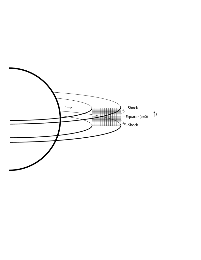
Figure 1: A diagram which indicates the geometry of the shocked-disk model (not-to-scale).

In our treatment, we use the functional forms of $\hat{f}$ and $\hat{g}$ for the temperature and density stratifications, respectively, as defined in Feldmeier et al. (1997) who considered plane parallel shock fronts. However, here the cooling layer above disk of Be stars is split into many concentric rings (e.g. $\sim$ 200 rings) along the disk radial extent and each ring is sliced into vertical sub-layers (e.g. $\sim$100 sub-layers), as is described in Fig. 1. Thus, each sub-layer has a specific density and temperature, which are assumed constant throughout the sub-layer. With these, one may obtain the emission measure for each ring and sub-layer from

$$\Delta(\mbox{$EM$})_{i}=n_{e}n_{p}\Delta V_{i}=\frac{\rho^{2}_{i}}{m^{2}_{H}\mu_{e}\mu_{p}}\Delta V_{i},$$ (10)

where $\Delta V_{i}$ and $\rho_{i}$ are the volume and mass density of the $i$th sub-layer, respectively. $\mu_{e}$ and $\mu_{p}$ are mean particle weights per electron and proton, respectively. Then, the X-ray emission from each ring and sub-layer is given (with $\Delta V_{i}=2\pi r_{i}\Delta z_{i}\Delta r_{i}$) by

$$\Delta L_{\nu,i}=\Delta(\mbox{$EM$})_{i}~{}\Lambda_{\nu}(T_{i}),$$ (11)

where $\Lambda_{\nu}(T_{i})$ is the cooling function at temperature $T$, frequency $\nu$ and chemical abundance (assumed solar), as given by Astrophysical Plasma Emission Database (APED) described by Smith et al. (1998).

The total X-ray emission for the entire shocked disk is found by summing the emission over all the rings and sub-layers and by multiplying by two to account for the upper and lower shock fronts of the disk,

$$L_{\nu}=2\sum_{i}\Delta L_{\nu,i}.$$ (12)

Integrating over the frequency range concerned, we obtain the X-ray luminosity

$$L_{x}=\int_{\nu_{1}}^{\nu_{2}}L_{\nu}d\nu,$$ (13)

where $\nu_{1}$ and $\nu_{2}$ are the lower and upper X-ray frequencies in the energy band of the instrument, such as 0.1 keV to 2.4 keV in the case of $ROSAT$, for example.

Calculations were carried out with sufficient numbers of rings and sub-layers so that the results were no longer dependent on the specific number of rings and sub-layers.

3 Effects of Model Parameters on X-ray Emission

The MTDGD models have been carried out for main sequence stars with given effective temperatures, mass loss rates, and terminal velocities. Our interest is in the X-ray properties at each spectral class as they are affected by the unknown wind velocity profiles, the stellar rotation rate and the magnetic fields. Thus, there are essentially three free parameters for any given spectral type, the $\beta$ value of the velocity law, the rotation rate parameter $S_{o}$, and the value of $\gamma$. For other properties that can affect the X-ray emission, such as the mass loss rate and terminal velocity, we choose values typical for each spectral type as in previous papers dealing with the MTD model.

Each of the three model parameters (i.e., $\beta$, $S_{o}$, and $\gamma$) affects the X-ray emission measure and $L_{x}/L_{B}$ ratio in different ways. To explain these various effects, we discuss the results from our modeling of the star $\zeta$ Oph, for which we find the following:

1. Changing the velocity law $\beta$ value can significantly affect the $L_{x}/L_{B}$ ratio. Changing $\beta$ has a small effect on the disk extent but it significantly affects the X-ray source as a result of the dependence of the cooling length on the wind velocity as parameterized with $\beta$. The cooling length depends on velocity as: $l_{c}\propto v_{w}^{4}/\rho_{s}\propto v_{w}^{5}$ (see Feldmeier et al. 1997). Therefore, the overall effect on the emission measure is $\mbox{$EM$}\propto\rho_{s}^{2}l_{c}\propto\rho^{2}_{s}v_{w}^{4}/\rho_{s}\propto v^{3}_{w}$. If, for example, $\beta$ is increased, meaning that a more slowly accelerating wind is incident upon the disk, then the emission measure from shock regions becomes lower and in turn $L_{x}/L_{B}$ is made lower, as is shown in Figs 2 and 3 for various $\beta$.

2. Changing $\gamma$ also gives rise to a change in $L_{x}/L_{B}$. Increasing $\gamma$ leads to an increase in the radial extent of the disk, and the extension occurs primarily outwardly away from the star. Thus there is a greater radial range of emitting material channeled to the disk. In Fig. 2, we show the dependence of $L_{x}/L_{B}$ on the magnetic parameter $\gamma$.

3. Increasing the rotation rate parameter $S_{o}$ affects the $L_{x}/L_{B}$ in three ways: (a) while the rotation rate is smaller than a turn-over value (for example, for given values of $\beta=1$ and $\gamma=1.5$, this turn-over value is $S_{o}\sim 0.5$), the gravity darkening is negligible, so increasing rotation helps to form the disk. Hence, the greater the rotation rate the larger the amount of matter channeled to the disk; (b) as the rotation rate increases further, the disk inner radius gets closer to the star, therefore a slower and denser (so cooler) wind reaches the disk. Hence, we find a situation similar to that discussed above regarding the $\beta$ value, and $L_{x}/L_{B}$ actually decreases; (c) if $S_{o}$ is increased even further, beyond a turn-over value, the gravity darkening effect plays an important role in significantly reducing the mass flow to the disk from equatorial regions on the star, and of course $L_{x}/L_{B}$ decreases significantly. Figs 2 and 3 also show this trend for given $\gamma$ and $\beta$.

In the tentative test, we show that when determining the $L_{x}/L_{B}$ from the model, we have to assume two of the three free parameters fixed to some values, then find how the $L_{x}/L_{B}$ varies with the remained one and whether the value of the remained one is appropriate for given the observed value of $L_{x}/L_{B}$. Figs. 2 and 3 show the varying trends, and imply the probable values for these three free parameters. Strictly, the ranges of the parameters could only really be solved by using a search to define the surface in 3-D ($S_{o}$, $\gamma$ and $\beta$) space with which fits are acceptable. Such a search will be carried out in the future and it may be more tightly constrained by fitting not only the X-ray luminosity but also the X-ray spectral hardness. From the above results, we might derive for our program stars like $\zeta$ Oph a least square formula that would look like: $L_{x}=k*S_{o}^{p}\,\gamma^{q}\,\beta^{w}$, where constant $k$ is a certain fraction of the wind kinetic energy converted to X-rays and the precise amount depends on the spin rate $S_{o}$, B and $\beta$. By doing a numerical partial derivative for each power to fit our results, we would find the range of the three powers $p\sim 1-4$, $q\sim 5-8$, and $w\sim 2-5$, which shows $L_{x}$ seems to be super dependent on the value of $\gamma$. This may explain why we are able to fit all the stars so exactly by our model.

4 Model Calculations and Comparisons with Observations

The physical quantities of the 8 program stars are listed in Table 1. We ran several models with considerations and compared the results with observations. The comparisons are shown as follows.

4.1 Comparisons with $ROSAT$ observations

For all program stars, we took MTDGD models to compute $L_{x}$ in three energy bands of $ROSAT$: soft (0.1–0.4 keV), hard (0.5–2.0 keV) and entire (0.1–2.4 keV) and got the hardness ratio HR=(H-S)/(H+S), the emission measure, and the ratio of X-ray to bolometric luminosity log $L_{x}/L_{B}$, which can be compared with the $ROSAT$ observations. In these calculations, we can choose various parameters of $\beta$, $S_{o}$ and $\gamma$. But for simplicity, we always use the minimal magnetic fields to $\gamma$ as given by Cassinelli et al. (2002), then fix either $\beta$ or $S_{o}$ and let the other one be adjustable. Note, in fact, what we did is to adjust parameters $S_{o}$ and $\beta$ until the fit is perfect. Hence we are assuming the model and inferring a range in $S_{o}$ and $\beta$ that is acceptable.

From the calculations with the MTDGD model, we achieve the observed X-ray $L_{x}/L_{B}$ ratio, within the allowed range of adjustments of the model’s free parameters. In fitting the observed log $L_{x}/L_{B}$, we have taken into account the following two different approaches.

In the first approach, we use the observed projected velocity $v~{}\sin i$ and used the average value of $<{\rm sin}~{}i>$ for a random set of inclination angles to estimate a surface rotation speed. This allows us to estimate the rotation rate $S_{o}$ of each star. This kind of approach has been used by Chandrasekhar & Münch (1950) and later by many authors such as Porter (1996) to analyze the rotation of Be stars. Also in the first approach to comparing the models with observations, we used the threshold (i.e. minimal) magnetic field given by Cassinelli et al. (2002) as our tentative field strength. Thus, for this case, we have one adjustable parameter — the velocity law index $\beta$ — to provide a fit to the observations. As is seen in Table 2, with the exception of just one star, the value of $\beta$ needed for the program stars is larger than unity. These values correspond to slowly accelerating winds as compared with estimates of $\beta$ for spherical winds. The calculation results are shown in Table 2 in which we can see that the model results of the emission measure and $L_{x}/L_{B}$ fit the observations quite well for a given set of free parameters. We plot figures with $L_{x}/L_{B}$ versus spectral type as in Fig. 4 and $L_{x}/L_{B}$ versus magnetic field B and $S_{o}$ as in Fig. 5 in terms of the model results in Table 2. We also list the derived hardness ratio of X-rays with regards to certain disk properties in the table and find it marginally in agreement with observations. We see that the hardness ratio of $\zeta$ Oph ($HR_{t}=0.630$) fit the observation ($HR_{o}=0.908$) marginally well. Unfortunately, the observational hardness ratios for other program stars are not available from $ROSAT$, but we still list the model results in the table for comparisons in the future.

As a second approach, we follow the radiative-driven wind theory and simply assume $\beta=1$, then we can fit the observed $L_{x}/L_{B}$ by adjusting the remaining parameter $S_{o}$. Note, the threshold field used here is determined by $\beta$ and $S_{o}$ for a given star as in Cassinelli et al. (2002). The calculation results are shown in Table 3 in which we can find that the range of $S_{o}$ for the various stars is from 0.49 to 0.88. This range is consistent with traditional values of the rotation rates for Be stars (Underhill & Doazan, 1982; Slettebak & Snow, 1987).

Thus we have found in using two approaches that the MTDGD models provide good fits to the X-ray observations. If one could find either a better way for estimating $S_{o}$ or $\beta$ for these channeled winds, then it would in principle be possible to derive new information on the process by which co-rotating magnetic fields actually produce disks. It is at least clear that the idea that angular momentum is transferred to disks by magnetic fields is broadly consistent, when Gravity Darkening is included, with the X-ray observations of Oe/Be stars.

4.2 Comparisons with $Chandra$ observations of $\zeta$ Oph

The Oe star $\zeta$ Oph has been observed at high spectral resolution with the $Chandra$ Satellite (Waldron 2005). The interpretation of the X-ray emission line profiles using emission line ratio diagnostics has led to a significantly improved understanding of the nature of the X-ray sources. This is especially in comparison with the information we had from earlier studies using low spectral resolution satellites. The observed line widths now provide information about the spread in line of sight velocities associated with the X-ray sources. The $f/i$ line ratios obtained from He-like ion $fir$ (forbidden, intercombination, resonance) emission lines provides a diagnostic of the radial locations of the shock source regions for these ions (e.g., Kahn et al. 2001; Waldron & Cassinelli 2001, 2007). Here we use the MTDGD model for $\zeta$ Oph to find the source region associated with the ion Mg XI and compare the line profile that would form in this region versus observations of the line from the $Chandra$ High Energy Transmission Grating Spectrometer (HETGS).

The primary goal of this exercise is to demonstrate that the MTDGD concept can reproduce the general properties of the Mg XI $fir$ lines without adjusting fitting parameters. The MTDGD predicts that the Mg XI emitting region is an annular region above the disk at a determined radius where temperatures reach values of order 5 MK at which Mg XI can form. We find that this is at about 1.8 $R_{*}$. The model that is used to calculate the line profile assumes a ring of emission at 1.8 $R_{*}$ and uses the post-shock density and temperature at that location. For comparison, the MTDGD radial location is about 22% larger than the source location obtained by Gagne et al. (2005) (1.2 to 1.4 $R_{*}$) in their model of the young magnetic O-star $\theta^{1}$ Ori C. From model predictions from Table 2, we know the value of $S_{o}$ and thus the angular speed at the Mg XI formation region. From Table 1 we know the value of $v~{}\sin i$ of the surface. Thus we can use the observed line width, assumed to be from the orbital velocity of the source region to derive the inclination factor $\sin i$. This corresponds to an angle $i=53^{\circ}$. The predicted X-ray source temperature of the ring of emission is determined from equation 7 using the incident wind speed determined by $v_{\infty}$ from Table 1 and assuming $\beta=1.29$. This yields $\rm T=4.94$ MK, which is near the temperature of 5 MK at which the Mg XI ion has its maximum ion fraction.

A key feature of our model line calculations is that we include “real” temperature and density dependent line emissivities which means that there is only “one” normalization applied to the total line complex calculation (i.e., we do not apply individual line normalizations). Our emissivities are determined by the MEKAL plasma emission code (Mewe et al. 1995). The main advantage of this code is that it allows one to explore density sensitive lines which is an important aspect in studies of the He-like fir line formation process in early-type stars. It is well established that the observed behavior of the He-like $fir$ lines, in particular the relative strengths of the $i$- and $f$-lines (i.e., the $f/i$ line ratio), is not due to density effects, but instead is dependent on the strength of the EUV/UV photospheric flux (e.g., Kahn et al. 2001; Waldron & Cassinelli 2001, 2007). Although current emissivity codes do not provide a means for determining line emission dependencies on EUV/UV flux (as first demonstrated by Blumenthal et al. 1972), one of us (Waldron) developed a special algorithm to simulate the $f/i$ ratio dependence on EUV/UV. Since we know how the $f/i$ ratio dependence separately on density and on EUV/UV flux, by equating these two relationships we can determine, what we call, an “effective EUV density” for any radial wind location for a given input photospheric EUV/UV flux. This effective EUV density is then used in the MEKAL code to determine the relative strengths of the $i$- and $f$-lines. We point out that the actual value of this effective EUV density is “not” an actual physical density, it is only a parameter that is used to simulate the effects of the EUV/UV flux on the $f/i$ ratio.

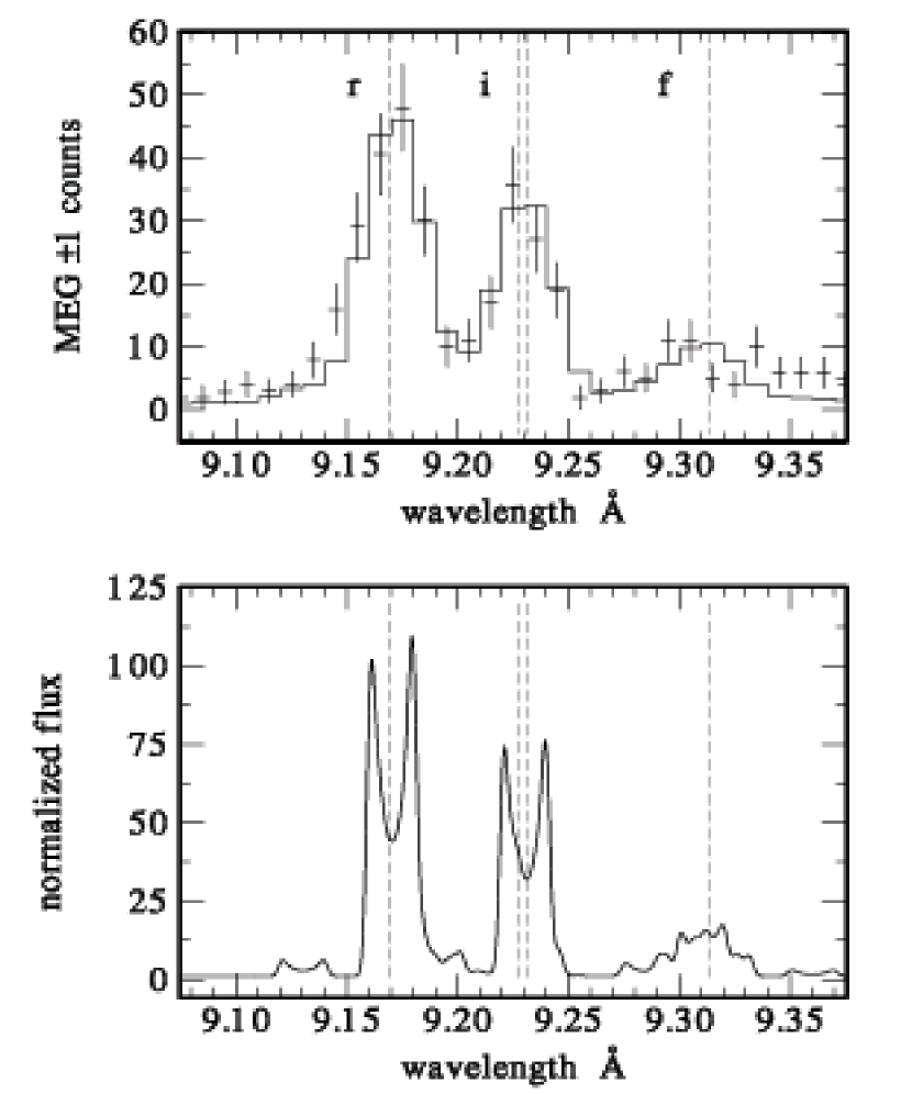
Figure 6: The top panel MTDGD model best fit to the $Chandra$ HETGS MEG +/-1 first order count spectrum of $\zeta$ Oph in the region of the He-like Mg XI $fir$ lines. The resultant chi-square to the number of degrees of freedom (DOF), i.e., $\chi^{2}$/DOF , is equal to 33.1/30. The bottom panel shows the predicted MTDGD model normalized observed flux that was used to generate the model count spectrum (top panel). The characteristic double peaked lines expected from a disk-type structure are clearly evident in the $r$- and $i$-lines. The $f$- line shows the effect of several weaker satellite lines. The vertical lines show the rest wavelengths of the $r$-, $i$-, and $f$-lines.

The model Mg XI $fir$ emission lines are calculated by a simple $\phi$ integration since the radial position of the emission zone is fixed. The emission is attenuated by the radial and $\phi$ dependent line-of-sight cool stellar wind X-ray continuum optical depth through the disk, including the effects of stellar occultation. The model X-ray emission includes all emissivities in a given wavelength region, e.g., the $fir$ lines, their satellite lines, any other lines that may be present, and the continuum. Once we specify the location and temperature of the disk distributed X-ray plasma (as determined by the MTDGD model), along with the effective EUV density as determined by a known photospheric flux, there is basically only one single free parameter, the normalization factor obtained from the fit which gives the total emission measure of the integrated disk distributed X-ray sources (i.e., a measure of $n_{e}^{2}$ times the volume of the X-ray emitting plasma). The predicted HETGS MEG+/-1 counts are compared to the observed counts in the top panel of Fig. 6 (using a bin size of 0.01 $\rm{\AA}$). The bottom panel of Fig. 6 shows the predicted input normalized model flux used to generate the model MEG+/-1 first order counts by using the extracted Ancillary Response File (ARF) and Redistribution Matrix File (RMF) appropriated for the $\zeta$ Oph data. The most obvious feature seen in the $r$- and $i$-lines is the characteristic double peaked line as expected from viewing a disk collection of sources seen at a large inclination angle. Since there is no radial velocity component in our model, the blue and red peaks should have the same strength. However, we see that the red peak of the $r$-line is slightly larger than the blue peak, which we attribute to the presence of several weaker satellite lines red-ward of the $r$-line. The most notable effect of other lines is seen in the vicinity of the $f$-line where we see that the double-peaked characteristic in the $f$-line is masked by these other lines. We also see that there is a slight emission excess on the blue-side of the $r$-line profile which suggests that the disk confined X-ray sources may have an outward radial velocity component of a few hundred $\rm{km\;s^{-1}}$, or perhaps the wind region above the disk might have standard radiation driven wind shocks that are contributing to the overall emission. Nevertheless, we conclude that the MTDGD model can reproduce the observed Mg XI $fir$ line shapes and line strengths, and more importantly, the model predicts an $f/i$ ratio that is very good agreement with the observations. Although this model fit to the HETGS data predicts a log EM of 54.52 which is approximately 40% larger than the observed emission measure derived from $ROSAT$ observations as listed in Table 2. An explanation for this small difference is that $\zeta$ Oph is a variable X-ray source (Waldron 2005) and at the time of the $Chandra$ observation the X-ray flux is about 40% larger than when the star was observed with $ROSAT$.

5 Discussion and Conclusions

The magnetically torqued disk model including gravity darkening effects or MTDGD, has here been tested to see if it can explain the basic X-ray properties of Oe/Be stars for which the model was developed. We had already found in the original papers on the MTD concept by Cassinelli et al. (2002) and Brown et al. (2004) that the idea of mass in Be disks is channeled by magnetic fields is consistent with the H$\alpha$ luminosities of Be stars and that the mass in the disks as derived from polarization observations is also explainable, though we again note that inclusion of $g_{z}$ will likely increase these in the model.

We have used a model that explains how matter can enter a disk with sufficient angular momentum to explain the quasi-Keplerian disks of Be stars, and the model uses field strengths that are comparable to those being found for other B stars. However an essential property of the MTDGD model is that it requires that X-rays be produced owing to the abrupt braking of the wind at the shock fronts. In summary, the paper contains several interesting results. (a) The paper tests the prediction that X-rays should be produced by the impact of channeled winds onto a disk. These X-rays would probably not be predicted from other current Be star models such as those in which the disk is produced by an extraction of angular momentum from the surface of a critically rotating star. (b) The model was based on the assumption that Be stars are rotating at their traditional values of about 70 percent critical and these rotation rates were found to be sufficient to explain the X-ray emission within the context of the MTD picture. (c) The model was found to require fields of order $10^{2}$ Gauss for Be stars, and our results show that these are adequate for the broad band X-ray production. (d) Broad band $ROSAT$ X-ray fluxes can be produced from B1 to B8 with MTDGD model parameters. (e) Fits are achievable even for the late B8 stars without invoking the presence of a dwarf M companion. (f) The model predicted that the Helium-like ion Mg XI had an $\rm R_{fir}$ about 1.8 stellar radii, which agrees well with where that line emission is expected to arise in $\zeta$ Oph with $Chandra$ observations, i.e., the $fir$ lines are predicted to occur there and to be broad, with a half width of about 400 $\rm{km\;s^{-1}}$ and the temperature structure is consistent with the formation of the Mg XI line.

Our discussion thus far has dealt with understanding the fundamental properties of Be stars as revealed by the $ROSAT$ and $Chandra$ observations. We have raised several questions during this paper that can now be addressed. (1) For our latest star B7 IVe, we found that the observed $ROSAT$ level of X-rays could be produced if the velocity law had value $\beta=0.77$. This small value for $\beta$ means that the channeled wind is colliding with the disk at a larger fraction of terminal wind speed than is the case for our other stars, which have $\beta$ values ranging from 1.3 to 2.8. The other required parameters for this star seem plausible: $B\sim 50$ Gauss, $S_{o}\sim 0.6$, (in the first of our two fitting procedures). Cohen et al. (1997) suggested that the emission measure needed to explain X-rays from late B stars were excessive, and that perhaps X-rays from magnetically confined region at the base of the wind are needed. So from our model of this star it appears that a magnetically confined X-ray formation region at the base is not needed. A bipolar magnetic field could instead just be torquing and channeling the wind toward the disk via X-ray emitting shocks. (2) The sharp drop-off of the X-ray luminosity beyond about B2 V, also seems to be explainable with a plausible range of our $\beta$, $S_{o}$, and magnetic field values of about 685 to 130 Gauss for our B2 and B3 stars.

It appears that the MTDGD model has the ability to answer two of the more difficult questions concerning existing X-ray observations of Be stars, with plausible parameters. The model can explain the X-ray luminosity across the B spectral band and it can explain reasonably well the observed line profile results from $Chandra$. Finally, it is important to note that our model results are not dependent on the nature of the high density regions on the equatorial plane for which there is controversy regarding field wrapping and magnetic breakouts. This is because our models are in effect providing information only about the X-ray formation regions at the boundaries of the disk, and the flow through these boundaries occurs before the matter reaches the cooled compressed region near the equatorial plane. We are not requiring that the gas be controlled by a strong field all the way to the equatorial plane, and in fact think that the gas is no longer dominated by the field in that region and is free to acquire a quasi-Keplerian orbital motion. The needed angular momentum had been transferred to the gas in the pre-shock magnetically torqued and channeled MTD flow.

Table 1: The Quantities of Program Stars

Star	Spectral	log$L_{B}$	$T_{e}$	$R_{\ast}$	$M_{\ast}$	$\dot{M}$	$v_{\infty}$	Distance	$v\sin i$
Name	Type	($L_{\odot}$)	(K)	($R_{\odot}$)	($M_{\odot}$)	($M_{\odot}$ yr-1)	(km s-1)	(pc)	(km s-1)
$\zeta$ Oph	O9.5 Vn	5.04	31600	8.00	25.0	$4.0\times 10^{-8}$	1500	154	385
$\kappa$ CMa	B1.5 IVe	4.21	24690	6.84	12.9	$4.2\times 10^{-9}$	1560	308	200
$\eta$ Cen	B1.5 Ve	3.99	24690	5.31	11.2	$1.5\times 10^{-9}$	1660	110	345
$\delta$ Cen	B2 IVe	4.01	23010	6.31	9.8	$2.0\times 10^{-9}$	1310	138	155
$\mu$ Cen	B2 IV-Ve	3.89	23010	5.50	10.4	$8.5\times 10^{-10}$	1470	163	180
$\alpha$ Ara	B2 Ve	3.77	23010	4.79	9.8	$4.5\times 10^{-10}$	1540	122	315
$\alpha$ Eri	B3 Ve	3.33	19320	4.07	6.9	$4.2\times 10^{-11}$	1330	27	250
$\alpha$ Col	B7 IVe	2.45	12790	3.39	3.7	$3.0\times 10^{-12}$	1250	44	210

Table 2: The Derived Quantities of Program Stars for a fixed value of $S_{o}$ and $\gamma$ with $\beta$ varied to fit the log $L_{x}/L_{B}$ ratio

							Theoretical			Observational
Star			B		$X_{i}$	$X_{o}$	log	log		log	log
Name	$\beta$	$S_{o}$	(Gauss)	$\gamma$	($R_{\ast}$)	($R_{\ast}$)	EMt	$L_{xt}/L_{B}$	HRt	EMo	$L_{xo}/L_{B}$
$\zeta$ Oph	1.29	0.64	2072	1.60	1.35	1.86	53.91	-7.47	0.630	54.30	-7.47
$\kappa$ CMa	2.43	0.42	917	2.09	1.78	2.47	52.65	-7.94	0.521	52.60	-7.94
$\eta$ Cen	1.53	0.69	514	1.39	1.28	1.81	51.99	-8.43	0.397	51.90	-8.42
$\delta$ Cen	2.81	0.36	684	2.42	1.98	2.77	51.90	-8.57	0.264	51.77	-8.57
$\mu$ Cen	1.34	0.38	685	2.77	1.91	2.55	53.07	-7.01	0.913	52.83	-7.01
$\alpha$ Ara	1.61	0.64	326	1.48	1.35	1.88	51.42	-8.78	0.358	51.33	-8.78
$\alpha$ Eri	1.45	0.56	130	1.78	1.47	2.01	50.80	-8.89	0.558	50.77	-8.89
$\alpha$ Col	0.77	0.59	44	1.95	1.42	1.89	50.41	-8.28	0.838	50.50	-8.28

Table 3: The Derived Quantities of Program Stars for a fixed value of $\beta$ and $\gamma$ with $S_{o}$ varied to fit the log $L_{x}/L_{B}$ ratio

							Theoretical			Observational
Star			B		$X_{i}$	$X_{o}$	log	log		log	log
Name	$\beta$	$S_{o}$	(Gauss)	$\gamma$	($R_{\ast}$)	($R_{\ast}$)	EMt	$L_{xt}/L_{B}$	HRt	EMo	$L_{xo}/L_{B}$
$\zeta$ Oph	1.0	0.752	1922	1.49	1.21	1.72	53.91	-7.47	0.636	54.30	-7.47
$\kappa$ CMa	1.0	0.821	604	1.38	1.14	1.68	52.65	-7.94	0.526	52.60	-7.94
$\eta$ Cen	1.0	0.879	477	1.30	1.09	1.66	51.98	-8.42	0.440	51.90	-8.42
$\delta$ Cen	1.0	0.815	392	1.38	1.15	1.68	51.90	-8.57	0.250	51.77	-8.57
$\mu$ Cen	1.0	0.495	546	2.21	1.60	2.11	53.08	-7.01	0.906	52.83	-7.01
$\alpha$ Ara	1.0	0.858	291	1.32	1.11	1.67	51.41	-8.78	0.390	51.33	-8.78
$\alpha$ Eri	1.0	0.725	112	1.54	1.24	1.74	50.81	-8.89	0.561	50.77	-8.89
$\alpha$ Col	1.0	0.488	50	2.24	1.61	2.13	50.41	-8.28	0.850	50.50	-8.28

Figure 2: The upper panel of the figure is the MTDGD model results for log $L_{x}/L_{B}$ versus magnetic field B (i.e. $\gamma$) in Gauss for $\zeta$ Oph stellar parameters and for $\beta=1$ with the various $S_{o}$ indicated in the figure. The curves show that log $L_{x}/L_{B}$ increases with increasing field strength. This is because larger magnetic fields give rise to more matter being torqued and channeled into the disk. Also note that as $S_{o}$ increases, log $L_{x}/L_{B}$ decreases and this is due to the gravity darkening effects. Note, the horizontal line in the figure indicates the observational value of log $L_{x}/L_{B}=-7.47$ for $\zeta$ Oph from $ROSAT$. The lower panel of the figure is the same as that in the upper panel but now $\beta=1.5$ instead.

Figure 3: The MTDGD model results of Log $L_{x}/L_{B}$ versus $S_{o}$ for a given magnetic field $B=1935$ Gauss (which corresponds to $\gamma=1.5$) as is needed for $\zeta$ Oph, and various $\beta$ indicated in the figure. The curves show that as $S_{o}$ initially increases from small values, the rotation helps to form the disk, and the larger the rotation rate the greater the X-ray emission. However, when $S_{o}$ is larger than a turn-over value, the gravity darkening plays a dominant role and leads to a decrease in the X-ray emission. Note also that $L_{x}/L_{B}$ tends to be larger for the smaller $\beta$ values, which correspond to faster wind impacting the inner parts of the disk. The horizontal line indicates the observational value of log $L_{x}/L_{B}=-7.47$ for $\zeta$ Oph as obtained from $ROSAT$.

Figure 4: Log $L_{x}/L_{B}$ versus spectral type. The model and observational results with opened circle for the former and filled triangle for the later, are plotted with the star names marked in the figure. The data used is from Table 2. Note, we actually adjust parameters $S_{o}$, $\gamma$, and $\beta$ until the fit is perfect so that we infer a range in $S_{o}$, $\gamma$, and $\beta$ that is acceptable.

Figure 5: The upper panel shows Log $L_{x}/L_{B}$ versus the magnetic fields needed to produce from the MTDGD models discussed in this paper. In the lower panel is shown the X-ray ratio versus the rotation rate parameter $S_{o}$ that we find is needed. The star names are marked in the figures. The B-star spectral type is included with each star’s name in parentheses. The data used is taken from Table 2. Note again we in fact adjust parameters $S_{o}$, $\gamma$, and $\beta$ in a range that is acceptable until the fit is perfect.

References

- Babel & Montmerle (1997) Babel, J. E., & Montmerle, T. 1997, A&A, 323, 121
- Baade & Ud-Doula (2005) Baade, D., & Ud-Doula, A. 2005, in ASP Conf. Ser. 337, the Nature and Evolution of Disks Around Hot Stars, ed. R. Ignace & K. G. Gayley, 129
- Berghöfer et al. (1996) Berghöfer , T. W., Schmitt, J. H. M. M., & Cassinelli, J. P. 1996, A&AS, 118, 481
- Bjorkman & Cassinelli (1993) Bjorkman, J. E., & Cassinelli, J. P. 1993, ApJ, 409, 429
- Blumenthal et al (1972) Blumenthal, G. R., Drake, G. W. F., & Tucker, W. H. 1972, ApJ, 172, 205
- Brown et al. (2004) Brown, J. C., Telfer, D., Li, Q., Hanuschik, R., Cassinelli, J. P., & Kholtygin, A. 2004, MNRAS, 252, 1061
- Brown & Cassinelli (2005) Brown, J. C., & Cassinelli, J. P. 2005, in ASP Conf. Ser. 337, the Nature and Evolution of Disks Around Hot Stars, ed. R. Ignace & K. G. Gayley, 88
- Cassinelli et al. (2002) Cassinelli, J. P., Cohen, D. H., MacFarlane, J. J., Sanders, W. T., & Welsh, B. Y. 1994, ApJ, 421, 705
- Cassinelli et al. (2001) Cassinelli, J. P., Miller, N. A., Waldron, W. L., MacFarlane, J. J., & Cohen, D. H. 2001, ApJ, 554, L55
- Cassinelli et al. (2002) Cassinelli, J. P., Brown, J. C., Maheswaran, M., Miller, N. A., & Telfer, D. C. 2002, ApJ, 578, 951
- Cassinelli et al. (2001) Cassinelli, J. P., Miller, N. A., Waldron, W. L., MacFarlane, J. J., & Cohen, D. H. 2001, ApJ, 554, L55
- Chandrasekhar & Münch (1950) Chandrasekhar, S. & Münch, G. 1950, ApJ, 111, 142
- Cohen et al. (1997) Cohen, D. H., Cassinelli, J. P., & Maheswaran, M. 1997, ApJ, 487, 867
- Cohen et al. (2003) Cohen, D. H., de Messieres, G. E., MacFarlane, J. J., Miller, N. A., Cassinelli, J. P., Owocki, S. P., & Liedahl, D. A. 2003, ApJ, 586, 495
- Doazan et al. (1991) Doazan, V., Sedmak, G., Barylak, M., & Rusconi, L. 1991, A Be Star Atlas of Far-UV and Optical High Resolution Spectra, ed. B. Batrick (ESA SP-1147)
- Donati et al. (2001) Donati, J. F., Wade, G. A., Babel, J., Henrichs, H. F., de Jong, J. A., Harries, T. J. 2001, MNRAS, 326, 1265
- Donati et al. (2002) Donati, J. Babel, J. Harries, T. J., Howarth, I.D., Petit, P., & Semel, M. 2002, MNRAS, 333, 55
- Fremat et al. (2005) Fremat Y., Zorec J.,Hubert, A. M., & Floquet M. 2005, arXiv:astro-ph/0503381
- Gagn et al (2005) Gagn, M., Oksala, M. E., Cohen, D. H., Tonnesen, S. K., ud-Doula, A., Owocki, S. P., Townsend, R. H. D., & MacFarlane, J. J. 2005, ApJ, 682, 586
- Hillier et al. (1993) Feldmeier, A., Kudritzki, R. P., Palsa, R., Pauldrach, A. W., & Puls, J. 1997, A&A, 320, 899
- Hanuschik et al. (1996) Hanuschik, R. W., Hummel, W., Sutorius, E., Dietle, O., & Thimm, 1996, A&AS, 116, 309
- Hillier et al. (1993) Hillier, D. J., Kudritzki, R. P., Pauldrach, A. W., Baade, D., Cassinelli, J. P., Puls, J., & Schmitt, J. H. M. M. 1993, A&A, 276, 117
- Howarth & Prinja (1989) Howarth, I. D., & Prinja R. K. 1989, ApJS, 69, 527
- Kahn et al (2001) Kahn, S. M., Leutenegger, M. A., Cottam, J., Rauw, G., Vreux, J. -M., den Boggende, A. J. F., Mewe, R., & Gudel, M. 2001, A&A, 365, L312
- Keppens & Goedbloed (1999) Keppens, R., Goedbloed, J. P. 1999, A&A, 343, 251
- Keppens & Goedbloed (2000) Keppens, R., Goedbloed, J. P., 2000, ApJ, 530, 1036
- Lamers & Cassinelli (1999) Lamers, H. G. J. L. M., & Cassinelli, J. P. 1999, Introduction to Stellar Winds (Cambridge: Cambidge Univ. Press), Ch. 9
- Lee et al. (1991) Lee, U., Saio, H., & Osaki, Y. 1991, MNRAS, 250, 432
- MacGregor (2003) MacGregor, K. B. & Cassinelli, J. P. 2003, ApJ, 586, 480
- Maheswaran (2003) Maheswaran, M. 2003, ApJ, 592, 1156
- Maheswaran & Cassinelli (1992) Maheswaran, M., & Cassinelli, J. C. P. 1994, ApJ, 386, 695
- Maheswaran & Cassinelli (1988) Maheswaran, M., & Cassinelli, J. C. P., 1988, ApJ, 335, 931
- Matt et al. (2000) Matt, S., Balick, B., Winglee, R., & Goodson, A. 2000, ApJ, 545, 965
- Mewe et al (1995) Mewe, R., Kaastra, J. S., & Liedahl, D. A. 1995, Legacy, Vol. 6 (HEASARC)
- Owocki, Cranmer, & Blondin (1994) Owocki, S. P., Cranmer, S. R., & Blondin, J. M. 1994, ApJ, 424, 887
- Owocki, Cranmer, & Gayley (1996) Owocki, S. P., Cranmer, S. R., & Gayley, K. G. 1996, ApJ, 472, L115
- Owocki, Townsend, & Ud-Doula (2005) Owocki, S., Townsend, R., & Ud-Doula, A. 2005, in AIP Conference Proceedings, Volume 784, MAGNETIC FIELDS IN THE UNIVERSE: From Laboratory and Stars to Primordial Structures, 239-252
- Owocki & ud-Doula (2003) Owocki, S. P., & ud-Doula, A. 2003, in ASP Conf. Ser. 305, Magnetic Fields in O, B,and A Stars: Origin and Connection to Pulsation, Rotation and Mass Loss, Ed. L. A. Balona, H. F. Henrichs, & R. Medupe (San Francisco: ASP), 350
- Pittard (2005) Pittard, J. M., Dobson, M. S., Durisen, R. H., Dyson, J. E., Hartquist, T. W., & O’Brien, J. T. 2005, A&A, 438, 11
- Porter (1996) Porter, J. M. 1996, MNRAS, 280, L31
- Quirrenbach (1997) Quirrenbach, A., Bjorkman, K. S., Bjorkman, J. E., Hummel, C. A., Buscher, D. F., Armstrong, J. T., Mozurkewich, D., Elias, N. M., II, & Babler, B. L. 1997, ApJ, 479, 477
- Slettebak & Snow (1987) Slettebak, A., & Snow, T. P. eds. 1987, IAU Colloq. 92, Physics of Be Stars (Cambridge: Cambridge Univ. Press)
- Smith et al. (1998) Smith, R. K., Brickhouse, N. S., Raymond, J. C., & Liedahl, D. A. 1998, in Proceedings of the First XMM Workshop on ”Science with XMM”, Noordwijk, The Netherlands: ESA
- Stelzer, et al. (2005) Stelzer, B., Flaccomio, E., Montmerle, T., Micela, G., Sciortino, S., Favata, F., Preibisch, T., & Feigelson, E. D. 2005, arXiv:astro-ph/0505503
- Struve (1931) Struve, O. 1931, ApJ, 73, 94
- Townsend et al. (2004) Townsend, R. H. D., Owocki, S. P., & Howarth, I. D. 2004, MNRAS, 350, 189
- Underhill & Doazan (1982) Underhill, A., & Doazan, V. eds. 1982, B Stars with and without Emission Lines (NASA SP-456, Washington: NASA)
- Waldron & Cassinelli (2001) Waldron, W. L., & Cassinelli, J. P. 2001, ApJ, 548, L45
- Waldron et al. (2004) Waldron, W. L., Cassinelli, J. P., Miller, N. A., MacFarlane, J. J., & Reiter, J. C. 2004, ApJ, 616, 542
- Waldron et al. (2005) Waldron, W. L. 2005, in ASP Conf. Ser., 337, the Nature and Evolution of Disks Around Hot Stars, Ed. R. Ignace & K. G. Gayley, 329
- Waldron & Cassinelli (2007) Waldron, W. L., & Cassinelli, J. P. 2007, ApJ, in press
- Wood et al. (1997) Wood, K., Bjorkman, K. S., & Bjorkman, J. E. 1997, ApJ, 477, 926
- Von Zeipel (1924) Von Zeipel, H., 1924, MNRAS, 84, 665