On the Whitham Equations for the Defocusing Complex Modified KdV Equation

Abstract

We study the Whitham equations for the defocusing complex modified KdV (mKdV) equation. These Whitham equations are quasilinear hyperbolic equations and they describe the averaged dynamics of the rapid oscillations which appear in the solution of the mKdV equation when the dispersive parameter is small. The oscillations are referred to as dispersive shocks. The Whitham equations for the mKdV equation are neither strictly hyperbolic nor genuinely nonlinear. We are interested in the solutions of the Whitham equations when the initial values are given by a step function. We also compare the results with those of the defocusing nonlinear Schrödinger (NLS) equation. For the NLS equation, the Whitham equations are strictly hyperbolic and genuinely nonlinear. We show that the weak hyperbolicity of the mKdV-Whitham equations is responsible for an additional structure in the dispersive shocks which has not been found in the NLS case.

1 Introduction

In [11, 12], Pierce and Tian studied the self-similar solutions of the Whitham equations which describe the zero dispersion limits of the KdV hierarchy. The main feature of the Whitham equations for the higher members of the hierarchy, of which the KdV equation is the first member, is that these Whitham equations are neither strictly hyperbolic nor genuinely nonlinear. This is in sharp contrast to the case of the KdV equation whose Whitham equations are strictly hyperbolic and genuinely nonlinear . In this paper, we extend their studies to the case of the complex modified KdV equation, which is the second member of the defocusing nonlinear Schrödinger hierarchy. The Whitham equations for the defocusing NLS equation are strictly hyperbolic and genuinely nonlinear, and they have been studied extensively (see for examples, [4, 6, 7, 10, 13]). However, for the mKdV equation, the Whitham equations are neither strictly hyperbolic nor genuinely nonlinear.

Let us begin with a brief description of the zero dispersion limit of the solution of the NLS equation

$$\sqrt{-1}\ \epsilon\frac{\partial\psi}{\partial t}+2\epsilon^{2}\frac{\partial^{2}\psi}{\partial x^{2}}-4|\psi|^{2}\psi=0\ ,$$ (1)

with the initial data

$$\psi(x,0)=A_{0}(x)\exp\left(\sqrt{-1}\ \frac{S_{0}(x)}{\epsilon}\right)\ .$$

Here $A_{0}(x)$ and $S_{0}(x)$ are real functions that are independent of $\epsilon$. Writing the solution $\psi(x,t;\epsilon)=A(x,t;\epsilon)\exp\left(\sqrt{-1}\ \frac{S(x,t;\epsilon)}{\epsilon}\right)$, and using the notation $\rho(x,t;\epsilon)=A^{2}(x,t;\epsilon)$, $v(x,t;\epsilon)={\partial S(x,t,\epsilon)/\partial x}$, one obtains the conservation form of the defocusing NLS equation

$$\left\{\begin{array}[]{lllll}&\displaystyle{\frac{\partial\rho}{\partial t}+\frac{\partial}{\partial x}(4\rho v)}=0\ ,\\ &\displaystyle{\frac{\partial}{\partial t}(\rho v)+\frac{\partial}{\partial x}\left(4\rho v^{2}+2\rho^{2}\right)=\epsilon^{2}\frac{\partial}{\partial x}\left(\rho\frac{\partial^{2}}{\partial x^{2}}\ln\rho\right)}\ .\end{array}\right.$$ (2)

The mass density $\rho=|\psi|^{2}$ and momentum density $\rho v=\frac{\sqrt{-1}}{2}(\psi\psi^{*}_{x}-\psi^{*}\psi_{x})$ have weak limits as $\epsilon\rightarrow 0$ [6]. These limits satisfy a $2\times 2$ system of hyperbolic equations

$$\left\{\begin{array}[]{lllll}&\displaystyle{\frac{\partial\rho}{\partial t}+\frac{\partial}{\partial x}(4\rho v)}=0\ ,\\ &\displaystyle{\frac{\partial}{\partial t}(\rho v)+\frac{\partial}{\partial x}\left(4\rho v^{2}+2\rho^{2}\right)=0}\ ,\end{array}\right.$$ (3)

until its solution develops a shock. System (3) can be rewritten in the diagonal form for $\rho\neq 0$,

$$\frac{\partial}{\partial t}\begin{pmatrix}{\alpha}\\ {\beta}\end{pmatrix}+2\begin{pmatrix}3{\alpha}+{\beta}&0\\ 0&{\alpha}+3{\beta}\end{pmatrix}\frac{\partial}{\partial x}\begin{pmatrix}{\alpha}\\ {\beta}\end{pmatrix}=0\ ,$$ (4)

where the Riemann invariants ${\alpha}$ and ${\beta}$ are given by

$$\alpha={v\over 2}+\sqrt{\rho}\ ,\quad\beta={v\over 2}-\sqrt{\rho}\ .$$ (5)

As a simple example, we consider the case with $\alpha=a=$constant. System (4) reduces to a single equation

$$\frac{\partial\beta}{\partial t}+2(a+3\beta)\frac{\partial\beta}{\partial x}=0\,.$$ (6)

The solution is given by the implicit form

$$\beta(x,t)=f(x-2(a+3\beta)t)\ ,$$

where $f(x)=\beta(x,0)$ is the initial data for $\beta$. One can easily see that if $\beta(x,0)$ decreases in some region, then $\beta(x,t)$ develops a shock in a finite time, i.e., $\partial\beta/\partial x$ becomes singular.

After the shock formation in the solution of (3) or (4), the weak limits are described by the NLS-Whitham equations, which can also be put in the Riemann invariant form [4, 6, 7, 10]

$$\frac{\partial u_{i}}{\partial t}+\lambda_{g,i}(u_{1},\ldots,u_{2g+2})\frac{\partial u_{i}}{\partial x}=0\ ,\quad i=1,2,\ldots,{2g+2}\ ,$$ (7)

where $\lambda_{g,i}$ are expressed in terms of complete hyperelliptic integrals of genus $g$ [8]. Here the number $g$ is exactly the number of phases in the NLS oscillations with small dispersion. Accordingly, the zero phase $g=0$ corresponds to no oscillations, and single and higher phases $g\geq 1$ correspond to the NLS oscillations. System (4) is viewed as the zero phase Whitham equations. The solution of the Whitham equations (7) for $g\geq 1$ then describes the averaged motion of the oscillations appearing in the solution of (1) (see e.g. [7]).

Let us discuss the most important $g=1$ case in more detail. We note that it is well known that the KdV oscillatory solution, in the single phase regime, can be approximately described by the KdV periodic solution when the dispersive parameter is small [1, 5, 16]. It is very possible to use the method of [1, 16] to show that the solution of the NLS equation (1) for small $\epsilon$ can be approximately described, in the single phase regime, by the periodic solution of the NLS equation. The NLS periodic solution has the form

$$\tilde{\rho}(x,t;\epsilon)=\rho_{3}+(\rho_{2}-\rho_{3})\,{\rm sn}^{2}(\sqrt{\rho_{1}-\rho_{3}}\,\theta(x,t;\epsilon),s)\,.$$ (8)

with $\theta(x,t;\epsilon)=(x-V_{1}t)/\epsilon$ and the velocity $V_{1}=V_{1}(\rho_{1},\rho_{2},\rho_{3})$. Here $\rho_{i}$’s are determined by the equation obtained from (2)

$$\frac{\epsilon^{2}}{4}\left(\frac{d\rho}{d\theta}\right)^{2}=(\rho-\rho_{1})(\rho-\rho_{2})(\rho-\rho_{3})\,$$

with $\rho_{1}>\rho_{2}>\rho_{3}$, and ${\rm sn}(z,s)$ is the Jacobi elliptic function with the modulus $s=(\rho_{2}-\rho_{3})/(\rho_{1}-\rho_{3})$. We can also write $\rho_{i}$’s as [3]

$$\left\{\begin{array}[]{lll}&\displaystyle{\rho_{1}=\frac{1}{4}(u_{1}+u_{2}-u_{3}-u_{4})^{2}}\\ &\displaystyle{\rho_{2}=\frac{1}{4}(u_{1}-u_{2}+u_{3}-u_{4})^{2}}\\ &\displaystyle{\rho_{3}=\frac{1}{4}(u_{1}-u_{2}-u_{3}+u_{4})^{2}}\end{array}\right.$$ (9)

with $u_{1}>u_{2}>u_{3}>u_{4}$. The velocity $V_{1}$ is then given by

$$V_{1}=2(u_{1}+u_{2}+u_{3}+u_{4})\,.$$

For constants $u_{1}$, $u_{2}$, $u_{3}$ and $u_{4}$, formula (8) gives the well known elliptic solution of the NLS equation. To describe the solution $\rho(x,t;\epsilon)$ of the NLS equation (2), the quantities $u_{1}$, $u_{2}$, $u_{3}$ and $u_{4}$ are instead functions of $x$ and $t$ and they evolve according to the single phase Whitham equations (7) for $g=1$.

The weak limit of $\rho(x,t;\epsilon)$ of NLS equation (1) as $\epsilon\rightarrow 0$ can be expressed in terms of $\rho_{1}$, $\rho_{2}$, $\rho_{3}$ and $\rho_{4}$ [6]

$$\overline{\rho(x,t)}=\rho_{1}-(\rho_{1}-\rho_{3})\frac{E(s)}{K(s)}\,,$$ (10)

where $K(s)$ and $E(s)$ are the complete elliptic integrals of the first and second kind, respectively. This weak limit can also be viewed as the average value of the periodic solution $\tilde{\rho}(x,t;\epsilon)$ of (8) over its period $L=2\epsilon K(s)/\sqrt{\rho_{1}-\rho_{3}}$.

In order to see how a single phase Whitham solution appears, we consider the following step initial data for system (4)

$$\alpha(x,0)=a,\quad\beta(x,0)=\begin{cases}b,~{}~{}x<0\\ c,~{}~{}x>0\end{cases}\,,$$ (11)

where $a>b$, $a>c$, $b\neq c$. The solution of (4) develops a shock if and only if $b>c$ (cf. (6)). After the formation of a shock, the Whitham equations (7) with $g=1$ kick in. For instance, we consider the Whitham equations with the initial data [7]

$$u_{1}(x,0)=a,\quad u_{2}(x,0)=b,\quad u_{3}(x,0)=\begin{cases}b,~{}~{}x<0\\ c,~{}~{}x>0\end{cases},\quad u_{4}(x,0)=c.$$ (12)

Now notice that the Whitham equations (7) for $g=1$ with the initial data (12) can be reduced to a single equation $u_{3t}+\lambda_{1,3}(a,b,u_{3},c)u_{3x}=0$. The equation has a global self-similar solution, which is implicitly given by $x/t=\lambda_{3}(a,b,u_{3},c)$. The $x$-$t$ plane is then divided into three parts

$$(1)\ \frac{x}{t}<\gamma\ ,\quad(2)\ \gamma<\frac{x}{t}<2a+4b+2c\ ,\quad(3)\ \frac{x}{t}>2a+4b+2c\ ,$$

where $\gamma=2(a+b+2c)-8(a-c)(b-c)/(a+b-2c)$ (see (31) and (35) below for the derivation). The solution of system (4) occupies the first and third parts, i.e.,

• for $x/t<\gamma$,

  $${\alpha}(x,t)=a,\quad{\beta}(x,t)=b,$$

• for $x/t>2a+4b+2c$,

  $${\alpha}(x,t)=a,\quad{\beta}(x,t)=c\ .$$

The Whitham solution of (7) with $g=1$ lives in the second part, i.e.,

• for $\gamma<x/t<2a+4b+2c$,

  $$u_{1}(x,t)=a\ ,\quad u_{2}(x,t)=b\ ,\quad\frac{x}{t}=\lambda_{1,3}(a,b,u_{3},c)\ ,\quad u_{4}(x,t)=c\ ,$$

where the solution $u_{3}$ can be obtained as a function of the self-similarity variable $x/t$, if

$$\frac{\partial\lambda_{1,3}}{\partial u_{3}}(a,b,u_{3},c)\neq 0.$$

Indeed, it has been shown that the Whitham equations (7) are genuinely nonlinear [6, 7], i.e.,

$$\frac{\partial\lambda_{1,i}}{\partial u_{i}}(u_{1},u_{2},u_{3},u_{4})>0,\,\quad i=1,2,3,4,$$ (13)

for $u_{1}>u_{2}>u_{3}>u_{4}$. In Figure 1, we plot the self-similar solution of the Whitham equations (7) with $g=1$ for the NLS equation, and the corresponding periodic oscillatory solution (8) for the initial data (11) with $a=4,b=0$ and $c=-1$. The oscillations describe a dispersive shock of the NLS equation under a small dispersion. Note here that the oscillations have a uniform structure, which is due to an almost linear profile of the Whitham solution $u_{3}$. This will be seen to be in sharp contrast to the case of the mKdV equation, which we will discuss later (cf. Figure 2).

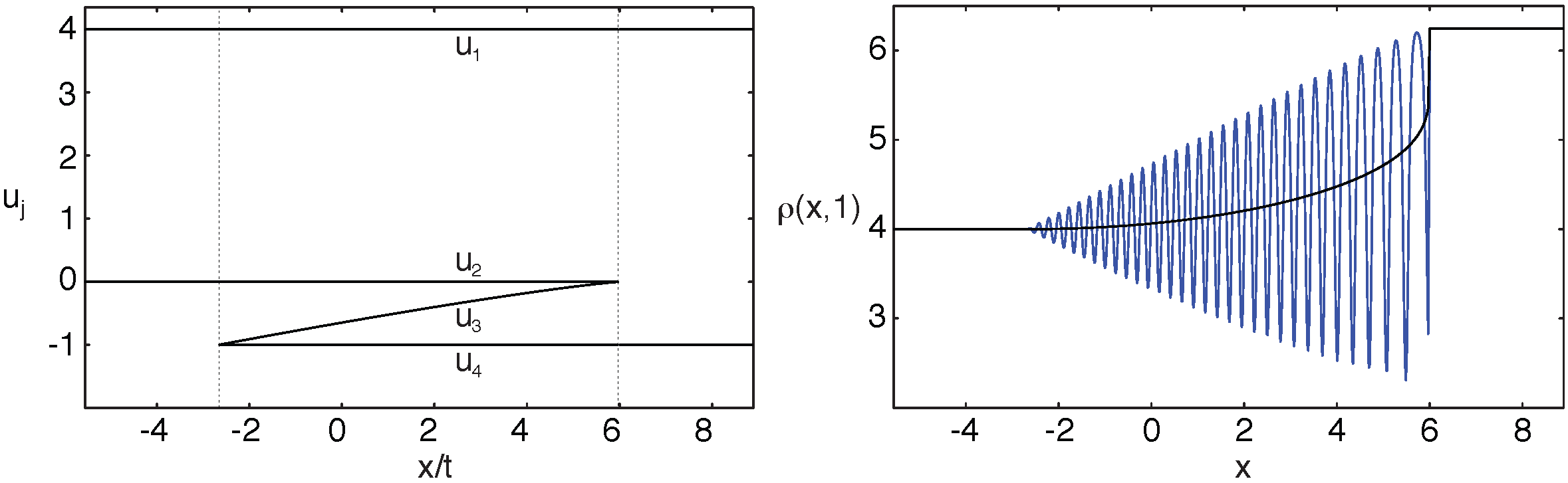
Fig. 1: Self-Similar solution of the NLS-Whitham equation (7) of $g=1$ and the corresponding oscillatory solution (8) of the NLS equation with $\epsilon=0.15$. The dark line in the middle of the oscillations is the weak limit $\overline{\rho(x,t)}$ given by (10). The initial data is given by (11) with $a=4$, $b=0$ and $c=-1$.

The figures in this paper all have the same form: On the left hand side is a plot of the solution of the Whitham equations as a function of the self-similarity variable $x/t$, which is exact, other than a numerical method used to implement the inverse function theorem. On the right hand side is the oscillatory solution given by (8) (respectively (21) for mKdV) at $t=1$, while the dark plot is the weak limit (10) of the oscillatory solution at $t=1$, both plots on the right are also exact. In the first two figures we demark the region where the Whitham equations with $g=1$ govern the solution, place a dashed-dotted line where the behavior of the oscillatory solution changes, and label the four functions $u_{1}>u_{2}>u_{3}>u_{4}$. The demarcation and labeling are similar in the other figures and we will leave them off for brevity. Although we do not include any numerical simulations, we would like to mention that E. Overman showed us his numerical simulation of the NLS and mKdV equations which captures the features of the oscillatory solutions plotted in this paper.

The defocusing NLS equation is just the first member of the defocusing NLS hierarchy; the second is the (defocusing) complex modified KdV (mKdV) equation

$${\partial\psi\over\partial t}+{3\over 2}\ |\psi|^{2}{\partial\psi\over\partial x}-{\epsilon^{2}\over 4}{\partial^{3}\psi\over\partial x^{3}}=0\ .$$ (14)

We again use $\psi(x,t;\epsilon)=A(x,t;\epsilon)\exp\left(\sqrt{-1}\ \frac{S(x,t;\epsilon)}{\epsilon}\right)$ and notation $\rho(x,t;\epsilon)=A^{2}(x,t;\epsilon)$, $v(x,t;\epsilon)={\partial S(x,t;\epsilon)/\partial x}$ to obtain the conservation form of the mKdV equation

$$\left\{\begin{array}[]{lllll}&\displaystyle{\frac{\partial\rho}{\partial t}+\frac{\partial}{\partial x}\left({3\over 4}\rho^{2}+{3\over 4}\rho v^{2}\right)={\epsilon^{2}}{\partial\over\partial x}\left(\rho^{3/4}{\partial^{2}\over\partial x^{2}}\rho^{1/4}\right)}\ ,\\ &\displaystyle{\frac{\partial}{\partial t}(\rho v)+\frac{\partial}{\partial x}\left({3\over 2}\rho^{2}v+{3\over 4}\rho v^{3}\right)=\frac{\epsilon^{2}}{4}\ \frac{\partial}{\partial x}\left[\frac{\partial^{2}}{\partial x^{2}}(\rho v)-{3\over 2}R\right]}\ ,\end{array}\right.$$ (15)

where

$$R=\frac{3v}{2\rho}\left(\frac{\partial\rho}{\partial x}\right)^{2}+\frac{\partial v}{\partial x}\frac{\partial\rho}{\partial x}-v\frac{\partial^{2}\rho}{\partial x^{2}}\,.$$

The mass density $\rho$ and momentum density $\rho v$ for the mKdV equation also have weak limits as $\epsilon\rightarrow 0$ [6]. As in the NLS case, the weak limits satisfy

$$\left\{\begin{array}[]{lllll}&\displaystyle{\frac{\partial}{\partial t}\rho+\frac{\partial}{\partial x}\left({3\over 4}\rho^{2}+{3\over 4}\rho v^{2}\right)=0}\ ,\\ &\displaystyle{\frac{\partial}{\partial t}(\rho v)+\frac{\partial}{\partial x}\left({3\over 2}\rho^{2}v+{3\over 4}\rho v^{3}\right)=0}\ ,\end{array}\right.$$ (16)

until the solution of (16) forms a shock. One can rewrite equations (16) as

$$\frac{\partial}{\partial t}\begin{pmatrix}\alpha\\ \beta\end{pmatrix}+\frac{3}{8}\begin{pmatrix}5\alpha^{2}+2\alpha\beta+\beta^{2}&0\\ 0&\alpha^{2}+2\alpha\beta+5\beta^{2}\end{pmatrix}\frac{\partial}{\partial x}\begin{pmatrix}\alpha\\ \beta\end{pmatrix}=0\ ,$$ (17)

where the Riemann invariants $\alpha$ and $\beta$ are again given by formula (5).

Let us again consider the simplest case $\alpha(x,0)=a$, where a is constant, to see how the solution of system (17) develops a shock. In this case, the system reduces to a single equation

$$\frac{\partial\beta}{\partial t}+\frac{3}{8}\left(a^{2}+2a\beta+5\beta^{2}\right)\frac{\partial\beta}{\partial x}=0\,.$$

As in the NLS case, we consider the initial function given by $\beta(x,0)=b$ for $x<0$ and $\beta(x,0)=c$ for $x>0$. We recall that, in the NLS case, the zero phase solution of (4) develops a shock if and only if $b>c$. However, the solution in the mKdV case develops a shock for $b>c$ if and only if $a+5b>0$. In addition, if $b<c$, the solution in the mKdV case develop a shock if and only if $a+5b<0$. These differences between the mKdV and NLS cases are due to the weak hyperbolicity of the system (17) (note that for the eigenspeed $\lambda=\frac{3}{8}(\alpha^{2}+2\alpha\beta+5\beta^{2})$ for $\beta$, we have $\partial\lambda/\partial\beta=\frac{3}{4}(\alpha+5\beta)$ which can change sign). As will be shown below, this leads to an additional structure in the dispersive shock for the mKdV case.

As in the case of the NLS equation, immediately after the shock formation in the solution of (16), the weak limits are described by the mKdV-Whitham equations

$$\frac{\partial u_{i}}{\partial t}+\mu_{g,i}(u_{1},\ldots,u_{2g+2})\frac{\partial u_{i}}{\partial x}=0\ ,\quad i=1,2,3\ldots,2g+2\ ,$$ (18)

where $\mu_{g,i}$’s can also be expressed in terms of complete hyperelliptic integrals of genus $g$ [6].

In this paper, we study the solution of the Whitham equations (18) with $g=1$ when the initial mass density $\rho(x,0)$ and momentum density $\rho(x,0)v(x,0)$ are step functions. In view of (5), this amounts to requiring $\alpha$ and $\beta$ of system (17) to have step-like initial data. We are interested in the following two cases:

• $\alpha(x,0)$ is a constant and

  $$\alpha(x,0)=a\ ,\quad\beta(x,0)=\left\{\begin{matrix}b,&x<0\\ c,&x>0\end{matrix}\right.\ ,\ \quad a>b\ ,a>c\ ,b\neq c\ ,$$ (19)

• $\beta(x,0)$ is a constant and

  $$\quad\alpha(x,0)=\left\{\begin{matrix}b,&x<0\\ c,&x>0\end{matrix}\right.\ ,\quad\beta(x,0)=a\ ,\quad b>a\ ,c>a\ ,b\neq c\ .$$ (20)

In the case of the NLS equation, the genuine nonlinearity of the single phase Whitham equations (see (13)) warrants that the solution is found by the implicit function theorem. However the mKdV-Whitham equations (18), in general, are not genuinely nonlinear, that is, a property like (13) is not available (see Lemma 1 below). Our construction of solutions of the Whitham equation (18) with $g=1$ makes use of the non-strict hyperbolicity of the equations. For the NLS case, it has been known in [6, 7] that the Whitham equations (7) with $g=1$ are strictly hyperbolic, that is,

$$\lambda_{1,1}>\lambda_{1,2}>\lambda_{1,3}>\lambda_{1,4}$$

for $u_{1}>u_{2}>u_{3}>u_{4}$. For the mKdV-Whitham equations (18) with $g=1$, the eigenspeeds $\mu_{1,i}(u_{1},u_{2},u_{3},u_{4})$ may coalesce in the region $u_{1}>u_{2}>u_{3}>u_{4}$ (we will discuss the details in Section 2).

Let us now describe one of our main results (see Theorem 3) for the single phase mKdV-Whitham equations with step-like initial function (19) for $a=4$, $b=1$ and $c=-1$. In this case, the space time is divided into four regions (see Figure 2) instead of three in the case of the NLS equation (cf. Figure 1)

$$(1)\ \frac{x}{t}<c_{1}\ ,\quad(2)\ c_{1}<\frac{x}{t}<c_{2}\ ,\quad(3)\ c_{2}<\frac{x}{t}<c_{3}\ ,\quad(4)\ \frac{x}{t}>c_{3}\ ,$$

where $c_{1}$, $c_{2}$ and $c_{3}$ are some constants. In the first and fourth regions, the solution of the $2\times 2$ system (17) governs the evolution:

• for $x/t<c_{1}$,

  $$\alpha(x,t)=4,\quad\beta(x,t)=1,$$

• for $x/t>c_{2}$,

  $$\alpha(x,t)=4,\quad\beta(x,t)=-1.$$

The Whitham solution of the $4\times 4$ system (18) with $g=1$ lives in the second and third regions;

• for $c_{1}<x/t<c_{2}$,

  $$u_{1}(x,t)=4,\quad u_{2}(x,t)=1,\quad\frac{x}{t}=\mu_{1,3}(4,1,u_{3},u_{4}),\quad\frac{x}{t}=\mu_{1,4}(4,1,u_{3},u_{4})\ ,$$

• for $c_{2}<x/t<c_{3}$,

  $$u_{1}(x,t)=4,\quad u_{2}(x,t)=1,\quad\frac{x}{t}=\mu_{1,3}(4,1,u_{3},-1)\ ,\quad u_{4}(x,t)=-1.$$

Note that, in the second region, we have

$$\mu_{1,3}(4,1,u_{3},u_{4})=\mu_{1,4}(4,1,u_{3},u_{4})$$

on a curve in the region $-1<u_{4}<u_{3}<4$. This implies the non-strict hyperbolicity of the mKdV-Whitham equations (18) for $g=1$.

It is again possible to use the method of [1, 16] to show that the solution of the mKdV equation (14) can be approximately described, in the single phase regime, by the periodic solution of the mKdV when $\epsilon$ is small. The periodic solution has the same form as (8) of the NLS, i.e.,

$$\tilde{\rho}(x,t;\epsilon)=\rho_{3}+(\rho_{2}-\rho_{3})\,{\rm sn}^{2}(\sqrt{\rho_{1}-\rho_{3}}\,\theta(x,t;\epsilon),s)\,.$$ (21)

However, $\theta(x,t;\epsilon)$ is now given by $\theta=(x-V_{2}t)/\epsilon$ with the velocity $V_{2}$ (see e.g. [9])

$$V_{2}=\frac{3}{8}\sigma_{1}^{2}-\frac{1}{2}\sigma_{2}\,,$$

where $\sigma_{1}=\sum_{j=1}^{4}u_{j}$ and $\sigma_{2}=\sum_{i<j}u_{i}u_{j}$ are the elementary symmetric functions of degree one and two, respectively. The functions $\rho_{1},\rho_{2}$ and $\rho_{3}$ are also given by formula (9). If $u_{1}$, $u_{2}$, $u_{3}$ and $u_{4}$ are constants, formula (21) gives the periodic solution of the mKdV equation. To describe the solution $\rho(x,t;\epsilon)$ of the mKdV equation (14), the quantities $u_{1}$, $u_{2}$, $u_{3}$ and $u_{4}$ must satisfy the single phase mKdV-Whitham equations (18) for $g=1$. The weak limit of $\rho(x,t;\epsilon)$ of the mKdV equation is also given by formula (10).

In Figure 2, we plot the self-similar solution of the Whitham equations (18) for $g=1$ and the corresponding periodic oscillatory solution (21). We note here that the pattern of the oscillation in this case has two distinct structures: one corresponds to the region (2), $c_{1}<x/t<c_{2}$, and the other corresponds to the region (3), $c_{2}<x/t<c_{3}$, We also note that the weak limit $\overline{\rho(x,t)}$ is not $C^{1}$ smooth at the boundary point $x/t=c_{2}\approx 4.63$.

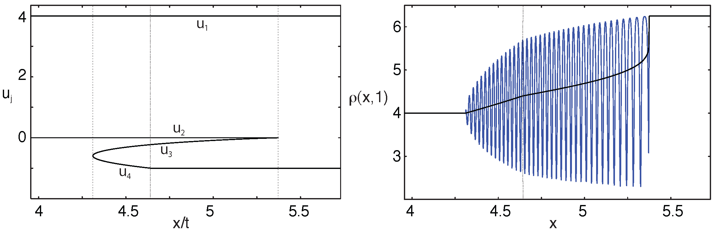
Fig. 2: Self-Similar solution of the mKdV-Whitham equation (18) with $g=1$ and the corresponding oscillatory solution (21) of the mKdV equation with $\epsilon=0.012$. The initial data is given by (19) with $a=4$, $b=0$ and $c=-1$. There are two distinct structures in the oscillations and they are separated by $x/t\approx 4.63$ (cf. Figure 1).

As we will show below, for other values of $a$, $b$ and $c$, the solutions of (17) and (18) with $g=1$ will be seen to be quite different from the above.

The Whitham equations (18) for the mKdV equation are analogous to the Whitham equations for the higher members of the KdV hierarchy [11, 12]. For step like initial data, the single phase Whitham solutions for the higher order KdV are also constructed using the non-strict hyperbolicity of the equations. In the case of strictly hyperbolic Whitham equations for the KdV, the oscillations (dispersive shock) have uniform structure. However, in the case of non-strict hyperbolic Whitham equations for the higher order KdV, an additional structure has been found in the dispersive shocks. This new structure is similar to the one found here in the dispersive shocks of the mKdV equation.

The organization of the paper is as follows. In Section 2, we will study the eigenspeeds, $\mu_{g,1},\mu_{g,2},\mu_{g,3}$ and $\mu_{g,4}$ of the Whitham equations (18) for $g=1$. In Section 3, we will construct the self-similar solutions of the single phase Whitham equations for the initial function (19) with $a>b>c$. In Section 4, we will construct the self-similar solution of the Whitham equations for the initial function (19) with $a>c>b$. In Section 5, we will briefly discuss how to handle the other step-like initial data (20).

2 The Whitham Equations

In this section we define the eigenspeeds $\lambda_{g,i}$’s and $\mu_{g,i}$’s of the Whitham equations (7) and (18) with $g=1$ for the NLS and the mKdV equations. For simplicity, we suppress the subscript $g=1$ in the notation $\lambda_{g,i}$’s and $\mu_{g,i}$’s in the rest of the paper.

We first introduce the polynomials of $\xi$ for $n=0,1,2,\dots$ [2, 4, 10]:

$$P_{n}(\xi,u_{1},u_{2},u_{3},u_{4})=\xi^{n+2}+a_{n,1}\xi^{n}+\dots+a_{n,n+2}\ ,$$ (22)

where the coefficients, $a_{n,1},a_{n,2},\dots,a_{n,n+2}$ are uniquely determined by the two conditions

$$\frac{P_{n}(\xi,u_{1},u_{2},u_{3},u_{4})}{\sqrt{(\xi-u_{1})(\xi-u_{2})(\xi-u_{3})(\xi-u_{4})}}=\xi^{n}+\mathcal{O}(\xi^{-2})\quad\mbox{for large $|\xi|$}$$

and

$$\int_{u_{2}}^{u_{1}}\frac{P_{n}(\xi,u_{1},u_{2},u_{3},u_{4})}{\sqrt{(u_{1}-\xi)(\xi-u_{2})(\xi-u_{3})(\xi-u_{4})}}d\xi=0\ .$$

The coefficients of $P_{n}$ can be expressed in terms of complete elliptic integrals.

The eigenspeeds of the Whitham equations (7) with $g=1$ for the NLS equation are defined in terms of $P_{0}$ and $P_{1}$ of (22) [4, 6, 10],

$$\lambda_{i}(u_{1},u_{2},u_{3},u_{4})=8\ \frac{P_{1}(u_{i},u_{1},u_{2},u_{3},u_{4})}{P_{0}(u_{i},u_{1},u_{2},u_{3},u_{4})}\ ,\quad i=1,2,3,4\ ,$$

which give

$$\lambda_{i}(u_{1},u_{2},u_{3},u_{4})=2\left(\sigma_{1}(u_{1},u_{2},u_{3},u_{4})-{I(u_{1},u_{2},u_{3},u_{4})\over\partial_{u_{i}}I(u_{1},u_{2},u_{3},u_{4})}\right)\,.$$ (23)

Here $\sigma_{1}:=\sum_{j=1}^{4}u_{j}$, and $I(u_{1},u_{2},u_{3},u_{4})$ is given by a complete elliptic integral [13]

$$I(u_{1},u_{2},u_{3},u_{4})=\int_{u_{2}}^{u_{1}}{d\eta\over\sqrt{(u_{1}-\eta)(\eta-u_{2})(\eta-u_{3})(\eta-u_{4})}}\ .$$ (24)

The function $I$ can be rewritten as a contour integral. Hence,

$$2(u_{i}-u_{j}){\partial^{2}I\over\partial u_{i}\partial u_{j}}={\partial I\over\partial u_{i}}-{\partial I\over\partial u_{j}}\ ,\quad i,j=1,2,3,4\$$ (25)

since the integrand satisfies the same equations for each $\eta\neq u_{i}$. This contour integral connection also allows us to give another formulation of $I$

$$I(u_{1},u_{2},u_{3},u_{4})=\int_{u_{4}}^{u_{3}}{d\eta\over\sqrt{(u_{1}-\eta)(u_{2}-\eta)(u_{3}-\eta)(\eta-u_{4})}}\ .$$ (26)

It follows from (23), (24) and (26) that

$$\lambda_{4}-2\sigma_{1}<\lambda_{3}-2\sigma_{1}<0<\lambda_{2}-2\sigma_{1}<\lambda_{1}-2\sigma_{1}$$ (27)

for $u_{4}<u_{3}<u_{2}<u_{1}$. This implies the strict hyperbolicity of the NLS-Whitham equation (7) for $g=1$.

The eigenspeeds $\lambda_{i}$’s have the following values [13]: At $u_{3}=u_{4}$, we have

$$\left\{\begin{array}[]{lll}\lambda_{1}=6u_{1}+2u_{2},\\ \lambda_{2}=2u_{1}+6u_{2},\\ \lambda_{3}=\lambda_{4}=2(u_{1}+u_{2}+2u_{4})-{8(u_{1}-u_{4})(u_{2}-u_{4})\over u_{1}+u_{2}-2u_{4}},\end{array}\right.$$ (31)

and at $u_{2}=u_{3}$,

$$\left\{\begin{array}[]{lll}\lambda_{1}=6u_{1}+2u_{4},\\ \lambda_{2}=\lambda_{3}=2u_{1}+4u_{3}+2u_{4},\\ \lambda_{4}=2u_{1}+6u_{4}.\end{array}\right.$$ (35)

Notice that the eigenspeed $\lambda_{2}=\lambda_{3}$ at $u_{2}=u_{3}$ is the same as the velocity of the periodic solution (8), i.e. $V_{1}=2\sigma_{1}=2(u_{1}+2u_{3}+u_{4})$.

The eigenspeeds of the mKdV-Whitham equations (18) with $g=1$ are [6]

$$\mu_{i}(u_{1},u_{2},u_{3},u_{4})=3\ \frac{P_{2}(u_{i},u_{1},u_{2},u_{3},u_{4})}{P_{0}(u_{i},u_{1},u_{2},u_{3},u_{4})}\ ,\quad i=1,2,3,4\ .$$ (36)

They can be expressed in terms of $\lambda_{1}$, $\lambda_{2}$, $\lambda_{3}$ and $\lambda_{4}$ of the NLS-Whitham equations (7) with $g=1$.

Lemma 1.

The eigenspeeds $\mu_{i}(u_{1},u_{2},u_{3},u_{4})$’s of (36) can be expressed in the form

$$\mu_{i}=\frac{1}{2}\left(\lambda_{i}-2\sigma_{1}\right)\frac{\partial q}{\partial u_{i}}+q\ ,\quad i=1,2,3,4\,,$$ (37)

where $\sigma_{1}=\sum_{j=1}^{4}u_{j}$ and $q=q(u_{1},u_{2},u_{3},u_{4})$ is the solution of the boundary value problem of the Euler-Poisson-Darboux equations

$$2(u_{i}-u_{j})\frac{\partial^{2}q}{\partial u_{i}\partial u_{j}} =\frac{\partial q}{\partial u_{i}}-\frac{\partial q}{\partial u_{j}}\ ,\quad i,j=1,2,3,4\ ,$$ (38)

$$q(u,u,u) =3u^{2}.$$

Also the $\mu_{i}$’s satisfy the over-determined systems

$$\frac{1}{\mu_{i}-\mu_{j}}\,{\partial\mu_{i}\over\partial u_{j}}=\frac{1}{\lambda_{i}-\lambda_{j}}\,{\partial\lambda_{i}\over\partial u_{j}}\,,\quad\quad i\neq j\ .$$ (39)

We omit the proof since it is very similar to the proof of an analogous result for the KdV hierarchy [14].

The boundary value problem (38) has a unique solution. The solution is a symmetric quadratic function of $u_{1}$, $u_{2}$, $u_{3}$ and $u_{4}$

$$q=\frac{3}{8}\sigma_{1}^{2}-\frac{1}{2}\sigma_{2}\ ,$$ (40)

where $\sigma_{2}=\sum_{i>j}u_{i}u_{j}$ is the elementary symmetric polynomial of degree two. Notice that $q$ gives the velocity of the periodic solution (21) for the mKdV equation, i.e. $V_{2}=q$.

For NLS, $\lambda_{i}$’s satisfy [13]

$$\frac{\partial\lambda_{4}}{\partial u_{4}}<\frac{3}{2}\frac{\lambda_{3}-\lambda_{4}}{u_{3}-u_{4}}<\frac{\partial\lambda_{3}}{\partial u_{3}}$$ (41)

for $u_{4}<u_{3}<u_{2}<u_{1}$. Similar results also hold for the mKdV-Whitham equations (18) with $g=1$.

Lemma 2.

$$\frac{\partial\mu_{3}}{\partial u_{3}} > \frac{3}{2}\ \frac{\mu_{3}-\mu_{4}}{u_{3}-u_{4}}\quad\mbox{if}\ \ \frac{\partial q}{\partial u_{3}}>0\ ,$$ (42)

$$\frac{\partial\mu_{4}}{\partial u_{4}} < \frac{3}{2}\ \frac{\mu_{3}-\mu_{4}}{u_{3}-u_{4}}\quad\mbox{if}\ \ \frac{\partial q}{\partial u_{4}}>0\ ,$$ (43)

for $u_{4}<u_{3}<u_{2}<u_{1}$.

Proof.

We use (37) and (41) to obtain

$$\frac{\partial\mu_{3}}{\partial u_{3}} =\frac{1}{2}\frac{\partial\lambda_{3}}{\partial u_{3}}\frac{\partial q}{\partial u_{3}}+\frac{1}{2}(\lambda_{3}-2\sigma_{1})\frac{\partial^{2}q}{\partial u_{3}^{2}}$$

$$>\frac{3}{4}\frac{\lambda_{3}-\lambda_{4}}{u_{3}-u_{4}}\frac{\partial q}{\partial u_{3}}+\frac{1}{2}(\lambda_{4}-2\sigma_{1})\frac{\partial^{2}q}{\partial u_{3}^{2}}\ ,$$ (44)

and

$$\mu_{3}-\mu_{4} =\frac{1}{2}\left(\lambda_{3}-\lambda_{4}\right)\frac{\partial q}{\partial u_{3}}+\frac{1}{2}(\lambda_{4}-2\sigma_{1})\left(\frac{\partial q}{\partial u_{3}}-\frac{\partial q}{\partial u_{4}}\right)$$

$$=\frac{1}{2}\left(\lambda_{3}-\lambda_{4}\right)\frac{\partial q}{\partial u_{3}}+(\lambda_{4}-2\sigma_{1})(u_{3}-u_{4})\frac{\partial^{2}q}{\partial u_{3}\partial u_{4}}$$

$$=\frac{2}{3}(u_{3}-u_{4})\left(\frac{3}{4}\,\frac{\lambda_{3}-\lambda_{4}}{u_{2}-u_{3}}\,\frac{\partial q}{\partial u_{3}}+\frac{3}{2}(\lambda_{4}-2\sigma_{1})\frac{\partial^{2}q}{\partial u_{3}\partial u_{4}}\right),$$ (45)

where we have used equation (38)

$$\frac{\partial q}{\partial u_{3}}-\frac{\partial q}{\partial u_{4}}=2(u_{3}-u_{4})\frac{\partial^{2}q}{\partial u_{3}\partial u_{4}}.$$

It follows from formula (40) for $q$ that

$$3\frac{\partial^{2}q}{\partial u_{3}\partial u_{4}}=\frac{\partial^{2}q}{\partial u_{3}^{2}}\ ,$$

which, along with with (44) and (45), proves (42). Inequality (43) is proved in the same way. ∎

The following calculations are useful in the subsequent sections. Using formula (37) for $\mu_{3}$ and $\mu_{4}$ and formulae (23) for $\lambda_{3}$ and $\lambda_{4}$, we obtain

$$\mu_{3}-\mu_{4} = {I\over(\partial_{u_{3}}I)(\partial_{u_{4}}I)}\left[{\partial q\over\partial u_{4}}{\partial I\over\partial u_{3}}-{\partial q\over\partial u_{3}}{\partial I\over\partial u_{4}}\right]$$ (46)

$$= {I\over(\partial_{u_{3}}I)(\partial_{u_{4}}I)}\left[{\partial q\over\partial u_{4}}({\partial I\over\partial u_{3}}-{\partial I\over\partial u_{4}})-({\partial q\over\partial u_{3}}-{\partial q\over\partial u_{4}}){\partial I\over\partial u_{4}}\right]$$

$$= {2I(u_{3}-u_{4})\over(\partial_{u_{3}}I)(\partial_{u_{4}}I)}\ M\ ,$$

where

$$M={\partial q\over\partial u_{4}}\ {\partial^{2}I\over\partial u_{3}\partial u_{4}}-{\partial^{2}q\over\partial u_{3}\partial u_{4}}\ {\partial I\over\partial u_{4}}\ .$$

Here we have used equations (25) for $I$ and equations (38) for $q$ in equality (46). Since $q$ of (40) is quadratic, we obtain

$${\partial M\over\partial u_{3}}={\partial q\over\partial u_{4}}\ {\partial^{3}I\over\partial u_{3}^{2}\partial u_{4}}\ .$$ (47)

We note that another expression for $M$ is

$$M={\partial q\over\partial u_{3}}\ {\partial^{2}I\over\partial u_{3}\partial u_{4}}-{\partial^{2}q\over\partial u_{3}\partial u_{4}}\ {\partial I\over\partial u_{3}}\ .$$

Hence, we get

$${\partial M\over\partial u_{4}}={\partial q\over\partial u_{3}}\ {\partial^{3}I\over\partial u_{3}\partial u_{4}^{2}}\ .$$ (48)

We next evaluate $M(u_{1},u_{2},u_{3},u_{4})$ when $u_{3}=u_{4}$. Using the integral formula (24) for the function I and applying the change of variable $\eta=(u_{1}-u_{2})\nu+u_{2}$, we obtain

$$M\Big{|}_{u_{3}=u_{4}} ={{\partial q\over\partial u_{4}}\over 4(u_{2}-u_{4})^{3}}\int_{0}^{1}{d\nu\over(1+{u_{1}-u_{2}\over u_{2}-u_{4}}\nu)^{3}\sqrt{\nu(1-\nu)}}$$

$$\phantom{=}-{{\partial^{2}q\over\partial u_{3}\partial u_{4}}\over 2(u_{2}-u_{4})^{2}}\int_{0}^{1}{d\nu\over(1+{u_{1}-u_{2}\over u_{2}-u_{4}}\nu)^{2}\sqrt{\nu(1-\nu)}}\ .$$

The two integrals can be evaluated exactly as

$$\int_{0}^{1}{d\nu\over(1+\gamma\nu)^{3}\sqrt{\nu(1-\nu)}}={\pi(8+8\gamma+3\gamma^{2})\over 8(1+\gamma)^{5\over 2}}\ ,\quad\int_{0}^{1}{d\nu\over(1+\gamma\nu)^{2}\sqrt{\nu(1-\nu)}}={\pi(2+\gamma)\over 2(1+\gamma)^{3\over 2}}$$

for $\gamma>-1$. We finally get

$$M\Big{|}_{u_{3}=u_{4}}={\pi U(u_{1},u_{2},u_{4})\over 128[(u_{2}-u_{4})(u_{1}-u_{4})]^{5\over 2}}\ ,$$ (49)

where

$$U(u_{1},u_{2},\xi) = [8(u_{2}-\xi)^{2}+8(u_{2}-\xi)(u_{1}-u_{2})+3(u_{1}-u_{2})^{2}](u_{1}+u_{2}+4\xi)$$ (50)

$$\quad-\ 8(u_{2}-\xi)[2(u_{2}-\xi)^{2}+3(u_{2}-\xi)(u_{1}-u_{2})$$

$$\quad\quad\quad+(u_{1}-u_{2})^{2}]\ .$$

Similar to (46) for $\mu_{3}$ and $\mu_{4}$, we have

$$\mu_{2}-\mu_{3}={2I(u_{2}-u_{3})\over(\partial_{u_{2}}I)(\partial_{u_{3}}I)}\ N\ ,$$ (51)

where

$$N={\partial q\over\partial u_{2}}\ {\partial^{2}I\over\partial u_{2}\partial u_{3}}-{\partial^{2}q\over\partial u_{2}\partial u_{3}}\ {\partial I\over\partial u_{2}}\ .$$

Since $q$ of (40) is quadratic, we obtain

$${\partial N\over\partial u_{3}}={\partial q\over\partial u_{2}}\ {\partial^{3}I\over\partial u_{2}\partial u_{3}^{2}}\ .$$ (52)

Finally, we use (31) and (37) to calculate

$$(\mu_{2}-\mu_{3})\Big{|}_{u_{3}=u_{4}} = {1\over 2}[\lambda_{2}-2(u_{1}+u_{2}+2u_{4})]{\partial q\over\partial u_{2}}-{1\over 2}[\lambda_{3}-2(u_{1}+u_{2}+2u_{4})]{\partial q\over\partial u_{3}}$$ (53)

$$= {(u_{2}-u_{4})\over 2(u_{1}+u_{2}-2u_{4})}\ V(u_{1},u_{2},u_{4})\ ,$$

where

$$V(u_{1},u_{2},u_{4})=3u_{1}^{2}+3u_{2}^{2}-12u_{4}^{2}+6u_{1}u_{2}+6u_{1}u_{4}-6u_{2}u_{4}\ .$$ (54)

3 Self-Similar Solutions

In this section, we construct self-similar solutions of the Whitham equations (18) with $g=1$ for the initial function (19) with $a>b>c$. The case with $a>c>b$ will be studied in next section. The solution of the zero phase Whitham equations (17) does not develop a shock when $a+5b\leq 0$. We are therefore only interested in the case $a+5b>0$.

We first study the $\xi$-zero of the cubic polynomial equation

$$U(a,b,\xi)=0\ ,$$ (55)

where $U$ is given by (50). It is easy to prove that for each pair of $a$ and $b$ satisfying $a>b$ and $a+5b>0$, $U(a,b,\xi)=0$ has only one simple real root. Denoting this zero by $\xi(a,b)$, we then deduce that $U(a,b,\xi)$ is positive for $\xi>\xi(a,b)$ and negative for $\xi<\xi(a,b)$. Since $U(a,b,-(a+b)/4)<0$ in view of (50), we must have

$$\xi(a,b)>-{a+b\over 4}\ .$$ (56)

For initial function (19) with $a>b>c$ and $a+5b>0$, we now classify the resulting Whitham solutions into four types:

• $~{}\xi(a,b)\leq c$ with any $a>b>c$

• $~{}\xi(a,b)>c$ with $a+5b>3(b-c)>0$

• $~{}\xi(a,b)>c$ with $a+5b=3(b-c)>0$

• $~{}\xi(a,b)>c$ with $0<a+5b<3(b-c)$

We will study the second type (II) first.

3.1 Type II

Here we consider the step initial function (19) satisfying $\xi(a,b)>c$ and $a+5b>3(b-c)>0$.

Theorem 3.

(see Figure 2.) For the step-like initial data (19) with $a>b>c$, $a+5b>3(b-c)$ and $\xi(a,b)>c$, the solution $(\alpha,\beta)$ of the zero phase Whitham equations (17) and the solution $(u_{1},u_{2},u_{3},u_{4})$ of the single phase Whitham equations (18) with $g=1$ are given as follows:

• For $x/t\leq\mu_{3}(a,b,\xi(a,b),\xi(a,b))$,

  $$\alpha=a\,,\quad\beta=b\,.$$ (57)

• For $\mu_{3}(a,b,\xi(a,b),\xi(a,b))<x/t<\mu_{3}(a,b,u^{**},c)$,

  $$u_{1}=a\ ,\quad u_{2}=b\ ,\quad\frac{x}{t}=\mu_{3}(a,b,u_{3},u_{4})\ ,\quad\frac{x}{t}=\mu_{4}(a,b,u_{3},u_{4})\ ,$$ (58)

  where $u^{**}$ is the unique solution $u_{3}$ of $\mu_{3}(a,b,u_{3},c)=\mu_{4}(a,b,u_{3},c)$ in the interval $c<u_{3}<b$.

• For $\mu_{3}(a,b,u^{**},c)\leq x/t<\mu_{3}(a,b,b,c)$,

  $$u_{1}=a\ ,\quad u_{2}=b\ ,\quad\frac{x}{t}=\mu_{3}(a,b,u_{3},c)\ ,\quad u_{4}=c.$$ (59)

• For $x/t\geq\mu_{3}(a,b,b,c)$,

  $$\alpha=a\,,\quad\beta=c.$$ (60)

The boundaries $x/t=\mu_{3}(a,b,\xi(a,b),\xi(a,b))$ and $x/t=\mu_{3}(a,b,b,c)$ are called the trailing and leading edges, respectively. They separate the solutions of the single phase Whitham equations (18) with $g=1$ and the zero phase Whitham equations (17). The single phase Whitham solution matches the zero phase Whitham solution in the following fashion (see Figure 1.):

$$(u_{1},u_{2}) = \mbox{the solution $(\alpha,\beta)$ of (\ref{mkdv0}) defined outside the region}\ ,$$ (61)

$$u_{3} = u_{4}\ ,$$ (62)

at the trailing edge;

$$(u_{1},u_{4}) = \mbox{the solution $(\alpha,\beta)$ of (\ref{mkdv0}) defined outside the region}\ ,$$ (63)

$$u_{2} = u_{3}\ ,$$ (64)

at the leading edge.

The proof of Theorem 3.1 is based on a series of lemmas: We first show that the solutions defined by formulae (58) and (59) indeed satisfy the Whitham equations (18) for $g=1$ [2, 15].

Lemma 4.

• The functions $u_{1}$, $u_{2}$, $u_{3}$ and $u_{4}$ determined by equations (58) give a solution of the Whitham equations (18) with $g=1$ as long as $u_{3}$ and $u_{4}$ can be solved from (58) as functions of $x$ and $t$.

• The functions $u_{1}$, $u_{2}$, $u_{3}$ and $u_{4}$ determined by equations (59) give a solution of the Whitham equations (18) with $g=1$ as long as $u_{3}$ can be solved from (59) as a function of $x$ and $t$.

Proof.

(1) $u_{1}$ and $u_{2}$ obviously satisfy the first two equations of (18) for $g=1$. To verify the third and fourth equations, we observe that

$$\frac{\partial\mu_{3}}{\partial u_{4}}=\frac{\partial\mu_{4}}{\partial u_{3}}=0$$ (65)

on the solution of (58). To see this, we use (39) to calculate

$$\frac{\partial\mu_{3}}{\partial u_{4}}={{\partial\lambda_{3}\over\partial u_{4}}\over\lambda_{3}-\lambda_{4}}\ (\mu_{3}-\mu_{4})=0\ .$$

The second part of (65) can be shown in the same way. We then calculate the partial derivatives of the third equation of (58) with respect to $x$ and $t$

$$1=\frac{\partial\mu_{3}}{\partial u_{3}}\ tu_{3x}\ ,\quad 0=\frac{\partial\mu_{3}}{\partial u_{3}}\ tu_{3t}+\mu_{3}\ ,$$

which give the third equation of (18) with $g=1$. The fourth equation of (18) with $g=1$ can be verified in the same way.

(2) The second part of Lemma 3.2 can easily be proved. ∎

We now determine the trailing edge. Eliminating $x$ and $t$ from the last two equations of (58) yields

$$\mu_{3}(a,b,u_{3},u_{4})-\mu_{4}(a,b,u_{3},u_{4})=0\ .$$ (66)

Since it degenerates at $u_{3}=u_{4}$, we replace (66) by

$$F(a,b,u_{3},u_{4}):={\mu_{3}(a,b,u_{3},u_{4})-\mu_{4}(a,b,u_{3},u_{4})\over u_{3}-u_{4}}=0\ .$$ (67)

Therefore, at the trailing edge where $u_{3}=u_{4}$, equation (67), in view of formulae (46) and (49), reduces to

$$U(a,b,u_{4})=0\ .$$ (68)

Noting that $\xi(a,b)$ is the unique solution of (55), we then deduce that $u_{4}=\xi(a,b)$.

Lemma 5.

Equation (67) has a unique solution satisfying $u_{3}=u_{4}$. The solution is $u_{3}=u_{4}=\xi(a,b)$. The rest of equations (58) at the trailing edge are $u_{1}=a$, $u_{2}=b$ and $x/t=\mu_{3}(a,b,\xi(a,b),\xi(a,b))$.

Having located the trailing edge, we now solve equations (58) in the neighborhood of the trailing edge. We first consider equation (67). We use (46) to write $F$ of (67) as

$$F(a,b,u_{3},u_{4})={2I\over(\partial_{u_{3}}I)(\partial_{u_{3}}I)}M(a,b,u_{3},u_{4})\ .$$

We note that at the trailing edge $u_{3}=u_{4}=\xi(a,b)$, we have $M(a,b,\xi(a,b),\xi(a,b))=0$ because of (49) and (68). We then use (47) and (48) to differentiate $F$ at the trailing edge

$${\partial F(a,b,\xi(a,b),\xi(a,b))\over\partial u_{3}} ={\partial F(a,b,\xi(a,b),\xi(a,b))\over\partial u_{4}}$$

$$={I\over 2(\partial_{u_{3}}I)(\partial_{u_{3}}I)}\ [a+b+4\xi(a,b)]\ {\partial^{3}I\over\partial u_{3}^{2}\partial u_{4}}>0\ ,$$

where we have used the expression (40) for $q$ in the last equation and (56) in the inequality. These show that equation (67) or equivalently (66) can be inverted to give $u_{4}$ as a decreasing function of $u_{3}$

$$u_{4}=A(u_{3})$$ (69)

in a neighborhood of $u_{3}=u_{4}=\xi(a,b)$.

We now extend the solution $A(u_{3})$ of equation (66) in the region $c<u_{4}<\xi(a,b)<u_{3}<b$ as far as possible. We first claim that

$${\partial q(a,b,u_{3},u_{4})\over\partial u_{3}}>0\ ,\quad{\partial q(a,b,u_{3},u_{4})\over\partial u_{4}}>0$$ (70)

on the extension. To see this, we first observe that inequalities (70) are true at the trailing edge $u_{3}=u_{4}=\xi(a,b)$. This follows from (40) and (56). Therefore, inequalities (70) hold in a neighborhood of the trailing edge. To prove that (70) remains true on the extension, we use formula (37) for $\mu_{3}$ and $\mu_{4}$ to rewrite equation (66) as

$${1\over 2}[\lambda_{3}-2(a+b+u_{3}+u_{4})]{\partial q\over\partial u_{3}}={1\over 2}[\lambda_{4}-2(a+b+u_{3}+u_{4})]{\partial q\over\partial u_{4}}\ .$$

Since the two terms in the two parentheses are both negative in view of (27) and since ${\partial q\over\partial u_{3}}-{\partial q\over\partial u_{4}}=(u_{3}-u_{4})/4>0$ in view of (40), neither ${\partial q\over\partial u_{3}}$ nor ${\partial q\over\partial u_{4}}$ can vanish on the extension. This proves inequalities (70).

We deduce from Lemma 2.2 that

$${\partial\mu_{3}\over\partial u_{3}}>0\ ,\quad{\partial\mu_{4}\over\partial u_{4}}<0$$ (71)

on the solution of (66). Because of (65) and (71), solution (69) of equation (66) can be extended as long as $c<u_{4}<\xi(a,b)<u_{3}<b$.

There are two possibilities: (1) $u_{3}$ touches $b$ before or simultaneously as $u_{4}$ reaches $c$ and (2) $u_{4}$ touches $c$ before $u_{3}$ reaches $b$. It follows from (35), (37) and (40) that

$$\mu_{3}(a,b,b,u_{4})-\mu_{4}(a,b,b,u_{4})={1\over 2}\ (b-u_{4})(a+2b+3u_{4})>0\quad\mbox{for $c\leq u_{4}<b$}\ ,$$ (72)

where we have used $a+2b+3c>0$ in the inequality. This shows that (1) is unattainable. Hence, $u_{4}$ will touch $c$ before $u_{3}$ reaches $b$. When this happens, equation (66) becomes

$$\mu_{3}(a,b,u_{3},c)=\mu_{4}(a,b,u_{3},c)\,.$$ (73)

Lemma 6.

Equation (73) has a simple zero in the interval $c<u_{3}<b$, counting multiplicities. Denoting the zero by $u^{**}$, then $\mu_{3}(a,b,u_{3},c)-\mu_{4}(a,b,u_{3},c)$ is positive for $u_{3}>u^{**}$ and negative for $u_{3}<u^{**}$.

Proof.

We use (46) and (47) to prove the lemma. In both formulae, $\partial_{u_{3}}I$, $\partial_{u_{4}}I$ and $\partial^{2}_{u_{3}u_{4}}I$ are all positive functions. By (47),

$${\partial M(a,b,u_{3},c)\over\partial u_{3}}={(a+b+u_{3}+3c)\over 4}{\partial^{3}I\over\partial u_{3}^{2}\partial u_{4}}\quad\ \mbox{for $c<u_{3}<b$}\ .$$ (74)

We claim that

$$M(a,b,u_{3},c)<0\quad\mbox{when $u_{3}=c$ ~{} ~{} and ~{} }~{}M(a,b,u_{3},c)>0\quad\mbox{for $u_{3}$ near $b$}\ .$$

The second inequality follows from (46) and (72). The first inequality can be deduced from formula (49)

$$M(a,b,c,c)={\pi U(a,b,c)\over 128[(b-c)(a-c)]^{5\over 2}}<0~{}~{}\quad\mbox{for $c<\xi(a,b)$}\ .$$

Therefore, $M(a,b,u_{3},c)$ has a zero in the interval $c<u_{3}<b$. The uniqueness of the zero follows from (74) in that $M(a,b,u_{3},c)$ increases or changes from decreasing to increasing as $u_{3}$ increases. This zero is exactly $u^{**}$ and the rest of the theorem can be proved easily. ∎

Having solved equation (66) for $u_{4}$ as a decreasing function of $u_{3}$ for $c<u_{4}<\xi(a,b)<u_{3}<b$, we turn to equations (58). Because of (65) and (71), the third equation of (58) gives $u_{3}$ as an increasing function of $x/t$, for $\mu_{3}(a,b,\xi(a,b),\xi(a,b))<x/t<\mu_{3}(a,b,u^{**},c)$. Consequently, $u_{4}$ is a decreasing function of $x/t$ in the same interval.

Lemma 7.

The last two equations of (58) can be inverted to give $u_{3}$ and $u_{4}$ as increasing and decreasing functions, respectively, of the self-similarity variable $x/t$ in the interval $\mu_{3}(a,b,\xi(a,b),\xi(a,b))<x/t<\mu_{3}(a,b,u^{**},c)$, where $u^{**}$ is given in Lemma 6.

We now turn to equations (59). We want to solve the third equation when $x/t>\mu_{3}(a,b,u^{**},c)$ or equivalently when $u_{3}>u^{**}$. According to Lemma 6, $\mu_{3}(a,b,u_{3},c)-\mu_{4}(a,b,u_{3},c)>0$ for $u^{**}<u_{3}<b$. In view of (70), ${\partial_{u_{3}}q}(a,b,u_{3},c)=(a+b+3u_{3}+c)/4$ is positive at $u_{3}=u^{**}$ and hence, it remains positive for $u_{3}>u^{**}$. By (42), we have

$${\partial\mu_{3}(a,b,u_{3},c)\over\partial u_{3}}>0\ .$$

Hence, the third equation of (59) can be solved for $u_{3}$ as an increasing function of $x/t$ as long as $u^{**}<u_{3}<b$. When $u_{3}$ reaches $b$, we have $x/t=\mu_{3}(a,b,b,c)$. We have therefore proved the following result.

Lemma 8.

The third equation of (59) can be inverted to give $u_{3}$ as an increasing function of $x/t$ in the interval $\mu_{3}(a,b,u^{**},c)\leq x/t\leq\mu_{3}(a,b,b,c)$.

We are ready to conclude the proof of Theorem 3.1. The solutions (57) and (60) are obvious. According to Lemma 3.5, the last two equations of (58) determine $u_{3}$ and $u_{4}$ as functions of $x/t$ in the region $\mu_{3}(a,b,\xi(a,b),\xi(a,b))\leq x/t\leq\mu_{3}(a,b,u^{**},c)$. By the first part of Lemma 3.2, the resulting $u_{1}$, $u_{2}$, $u_{3}$ and $u_{4}$ satisfy the Whitham equations (18) with $g=1$. Furthermore, the boundary conditions (61) and (62) are satisfied at the trailing edge $x=\mu_{3}(a,b,\xi(a,b),\xi(a,b))$.

Similarly, by Lemma 3.6, the third equation of (59) determines $u_{3}$ as a function of $x/t$ in the region $\mu_{3}(a,b,u^{**},c)\leq x/t\leq\mu_{3}(a,b,b,c)$. It then follows from the second part of Lemma 3.2 that $u_{1}$, $u_{2}$, $u_{3}$ and $u_{4}$ of (59) satisfy the Whitham equations (18) for $g=1$. They also satisfy the boundary conditions (63) and (64) at the leading edge $x/t=\mu_{3}(a,b,b,c)$. We have therefore completed the proof of Theorem 3.1.

A graph of the Whitham solution $(u_{1},u_{2},u_{3},u_{4})$ is given in Figure 2. It is obtained by plotting the exact solutions of (58) and (59).

3.2 Type I

Here we consider the initial function (19) satisfying $\xi(a,b)\leq c$ with $b>c$ and $a+5b>0$.

Fig. 3: Self-Similar solution of the Whitham equations (18) with $g=1$ and the corresponding oscillatory solution (21) of the mKdV equation with $\epsilon=0.07$. The initial data is given by (19) with $a=7$, $b=0$ and $c=-1$ of type I.

We will only present our proofs briefly, since they are, more or less, similar to those in Section 3.1. The main feature of this case is that the $\xi$-zero point does not appear in the solution $u_{3}$, and the Whitham equations (18) with $g=1$ are strictly hyperbolic on the solution.

Theorem 9.

(see Figure 3.) For the step-like initial data (19) with $a>b>c$, $a+5b>0$ and $\xi(a,b)\leq c$, the solution of the Whitham equations (18) with $g=1$ is given by

$$u_{1}=a\ ,\quad u_{2}=b\ ,\quad\frac{x}{t}=\mu_{3}(a,b,u_{3},c)\ ,\quad u_{4}=c$$

for $\mu_{3}(a,b,c,c)<x/t<\mu_{3}(a,b,b,c)$. Outside this interval, the solution of (17) is given by

$$\alpha=a\ ,\quad\beta=b~{}~{}\quad\mbox{for}\quad\frac{x}{t}\leq\mu_{3}(a,b,c,c)\,,$$

and

$$\alpha=a\ ,\quad\beta=c~{}~{}\quad\mbox{for}\quad\frac{x}{t}\geq\mu_{3}(a,b,b,c)\ .$$

Proof.

It suffices to show that $\mu_{3}(a,b,u_{3},c)$ is an increasing function of $u_{3}$ for $c<u_{3}<b$. Substituting (40) for $q$ into (47) yields

$${\partial M(a,b,u_{3},c)\over\partial u_{3}}={1\over 4}[a+b+u_{3}+3c]\ {\partial^{3}I\over\partial u_{3}^{2}\partial u_{4}}\geq{1\over 4}[a+b+4\xi(a,b)]\ {\partial^{3}I\over\partial u_{3}^{2}\partial u_{4}}>0$$

for $c<u_{3}<b$, where we have used $\xi(a,b)\leq c$ in the first inequality and (56) in the second one. We now use formula (49) to calculate the value of $M(a,b,u_{3},c)$ at $u_{3}=c$

$$M(a,b,c,c)={\pi U(a,b,c)\over 128[(b-c)(a-c)]^{5\over 2}}\geq 0\quad\mbox{for $\xi(a,b)\leq c$}\ ,$$

because $U(a,b,\xi)\geq 0$ for $\xi\geq\xi(a,b)$. Therefore, $M(a,b,u_{3},c)>0$ for $c<u_{3}<b$. It then follows from (46) that $\mu_{3}(a,b,u_{3},c)-\mu_{4}(a,b,u_{3},c)>0$. Since ${\partial q\over\partial u_{3}}(a,b,u_{3},c)=(a+b+3u_{3}+c)/4>(a+b+3\xi(a,b))/4>0$ because of (56), we conclude from Lemma 2.2 that

$${d\mu_{3}(a,b,u_{3},c)\over du_{3}}>0$$

for $c<u_{3}<b$. ∎

3.3 Type III

Here we consider the step initial function (19) satisfying $\xi(a,b)>c$ with $a+5b=3(b-c)>0$.

Fig. 4: Self-Similar solution of the Whitham equations (18) with $g=1$ and the corresponding oscillatory solution (21) of the mKdV equation with $\epsilon=0.007$. The initial data is given by (19) with $a=3$, $b=0$, $c=-1$ of type III.

Theorem 10.

(see Figure 4.) For the step-like initial data (19) with $a>b>c$, $\xi(a,b)>c$ and $a+5b=3(b-c)$, the solution of the $g=1$ Whitham equations (18) with $g=1$ is given by

$$u_{1}=a\ ,\quad u_{2}=b\ ,\quad\frac{x}{t}=\mu_{3}(a,b,u_{3},u_{4})\ ,\quad\frac{x}{t}=\mu_{4}(a,b,u_{3},u_{4})\,,$$

for $\mu_{3}(a,b,\xi(a,b),\xi(a,b))<x/t<\mu_{3}(a,b,b,c)$. Outside the region, the solution of equations (17) is given by

$$\alpha=a\ ,\quad\beta=b\,,\quad\mbox{for}\quad\frac{x}{t}\leq\mu_{3}(a,b,\xi(a,b),\xi(a,b))\,,$$

and

$$\alpha=a\ ,\quad\beta=c\,,\quad\mbox{for}\quad\frac{x}{t}\geq\mu_{3}(a,b,b,c)\ .$$

Proof.

It suffices to show that $u_{3}$ and $u_{4}$ of $\mu_{2}(a,b,u_{3},u_{4})-\mu_{3}(a,b,u_{3},u_{4})=0$ reaches $b$ and $c$, respectively, simultaneously. To see this, we deduce from the calculation (72) that

$$\mu_{3}(a,b,b,u_{4})-\mu_{4}(a,b,b,u_{4})={1\over 2}(b-u_{4})(a+2b+3u_{4})\ ,$$ (75)

vanishes at $u_{4}=(-a-2b)/3=c$. ∎

3.4 Type IV

Here we consider the step initial function (19) satisfying $\xi(a,b)>c$ with $0<a+5b<3(b-c)$.

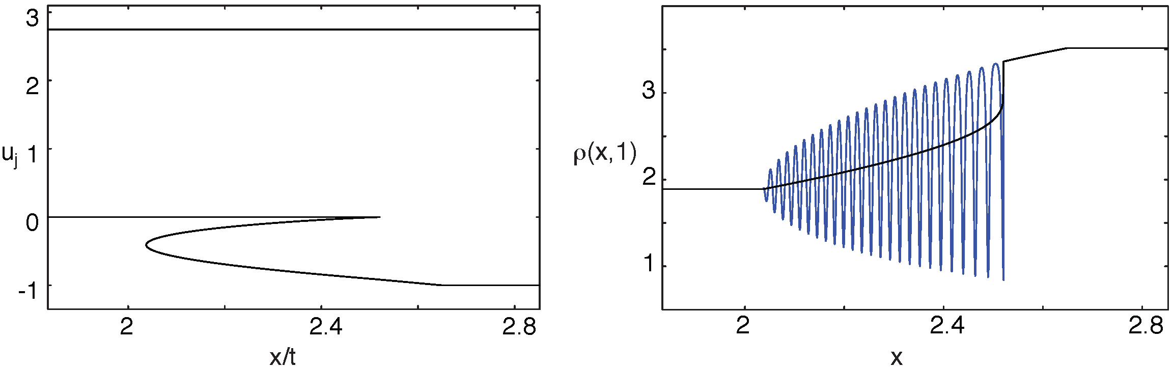
Fig. 5: Self-Similar solution of the Whitham equations (18) with $g=1$ and the corresponding oscillatory solution (21) of the mKdV equation with $\epsilon=0.006$. The initial data is given by (19) with $a=2.75$, $b=0$ and $c=-1$ of type IV. The solution in the region $2.52<x/t<2.65$ represents a rarefaction wave.

Theorem 11.

(see Figure 5.) For the step-like initial data (19) with $a>b>c$, $\xi(a,b)>c$ and $0<a+5b<3(b-c)$, the solution of the Whitham equations (14) is given by

$$u_{1}=a\ ,\quad u_{2}=b\ ,\quad\frac{x}{t}=\mu_{2}(a,b,u_{3},u_{4})\ ,\quad x=\mu_{3}(a,b,u_{3},u_{4})\ t$$

for $\mu_{3}(a,b,\xi(a,b),\xi(a,b))<x/t<\mu_{3}(a,b,b,-(a+2b)/3)$. Outside the region, the solution of equation (17) is divided into the three regions:

• For $x/t\leq\mu_{3}(a,b,\xi(a,b),\xi(a,b))$,

  $$\alpha=a\ ,\quad\beta=b\ .$$

• For $\mu_{3}(a,b,b,-(a+2b)/3)\leq\frac{x}{t}\leq\frac{3}{8}\left(a^{2}+2ac+5c^{2}\right)$,

  $$\alpha=a,\quad\beta=-\frac{1}{5}a-\sqrt{\frac{8}{15}\frac{x}{t}-\frac{4}{25}a^{2}}\ .$$

• For $x/t\geq\frac{3}{8}\left(a^{2}+2ac+5c^{2}\right)$,

  $$\alpha=a,\quad\beta=c\ .$$

Proof.

By the calculation (75), when $u_{3}$ of $\mu_{3}(a,b,u_{3},u_{4})-\mu_{4}(a,b,u_{3},u_{4})=0$ touches $b$, the corresponding $u_{4}$ reaches $-(a+2b)/3$, which is above $c$. Hence, equations

$$\frac{x}{t}=\mu_{3}(a,b,u_{3},u_{4})\ ,\quad\frac{x}{t}=\mu_{4}(a,b,u_{3},u_{4})$$

can be inverted to give $u_{3}$ and $u_{4}$ as functions of $x/t$ in the region $\mu_{3}(a,b,\xi(a,b),\xi(a,b))<x/t<\mu_{3}(a,b,b,-(a+2b)/3)$. In the region (2), the equations (17) has a rarefaction wave solution. ∎

4 More Self-Similar Solutions

In this section, we construct self-similar solutions of the $g=1$ Whitham equations (18) for the initial function (19) with $a>c>b$. The solution of equations (17) does not develop a shock for $a+5b\geq 0$. We are therefore only interested in the case $a+5b<0$. We classify the resulting Whitham solution into four types:

• $~{}a+5b\leq-4(c-b)<0$

• $~{}0>a+5b>-4(c-b)$ with $V(a,c,b)<0$

• $~{}0>a+5b>-4(c-b)$ with $V(a,c,b)=0$

• $~{}0>a+5b>-4(c-b)$ with $V(a,c,b)>0$

where $V$ is a quadratic polynomial given by (54).

4.1 Type V

Here we consider the step initial function (19) satisfying $a+5b\leq-4(c-b)<0$.

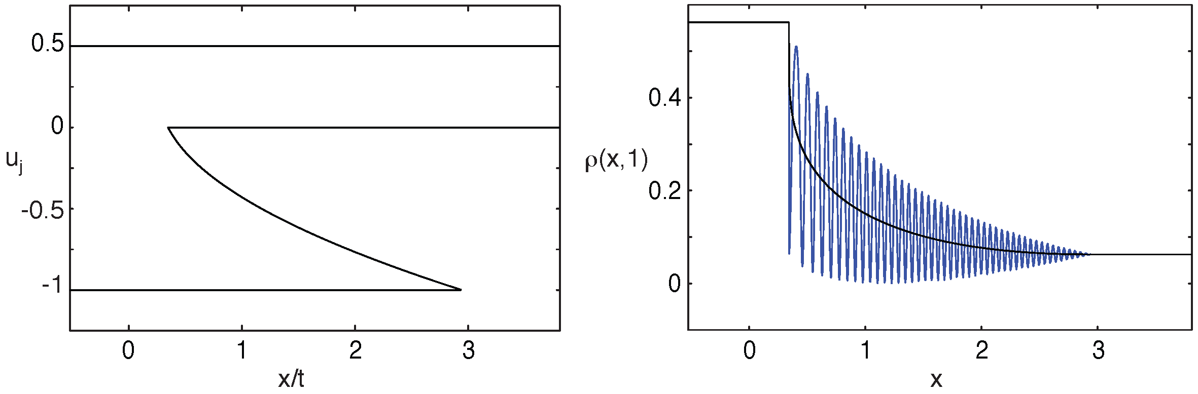
Fig. 6: Self-Similar solution of the Whitham equations (18) with $g=1$ and the corresponding oscillatory solution (21) of the mKdV equation with $\epsilon=0.018$. The initial data is given by (19) with $a=1/2$, $b=-1$ and $c=0$ of type V.

Theorem 12.

(see Figure 6.) For the step-like initial data (19) with $a>c>b$, $a+5b\leq-4(c-b)$, the solution of the Whitham equations (18) with $g=1$ is given by

$$u_{1}=a\ ,\quad u_{2}=c\ ,\quad\frac{x}{t}=\mu_{3}(a,c,u_{3},b)\ ,\quad u_{4}=b$$

for $\mu_{3}(a,c,c,b)<x/t<\mu_{3}(a,c,b,b)$. Outside this interval, the solution of (17) is given by

$$\alpha=a\,\quad\beta=b\quad\mbox{for}\quad\frac{x}{t}\leq\mu_{3}(a,c,c,b)\,,$$

and

$$\alpha=a\,\quad\beta=c\quad\mbox{for}\quad\frac{x}{t}\geq\mu_{3}(a,c,b,b)\ .$$

Proof.

It suffices to show that $\mu_{3}(a,c,u_{3},b)$ is a decreasing function of $u_{3}$ for $b<u_{3}<c$. By (37), we have

$${\partial\mu_{3}(a,c,u_{3},b)\over\partial u_{3}}={1\over 2}{\partial\lambda_{3}\over\partial u_{3}}{\partial q\over\partial u_{3}}+{1\over 2}[\lambda_{3}-2(a+c+u_{3}+b)]{\partial^{2}q\over\partial u_{3}^{2}}\ .$$

The second term is negative because of (27) and ${\partial^{2}q\over\partial u_{2}^{2}}=3/8>0$. The first term is also negative: Its first factor is positive in view of (13); while its second factor is

$${\partial q\over\partial u_{3}}={1\over 4}(a+c+3u_{3}+b)<0,$$

for $b<u_{3}<c$, as we have that $a+b+4c\leq 0$. ∎

4.2 Type VI

Here we consider the step initial function (19) satisfying $0>a+5b>-4(c-b)$ with $V(a,c,b)<0$.

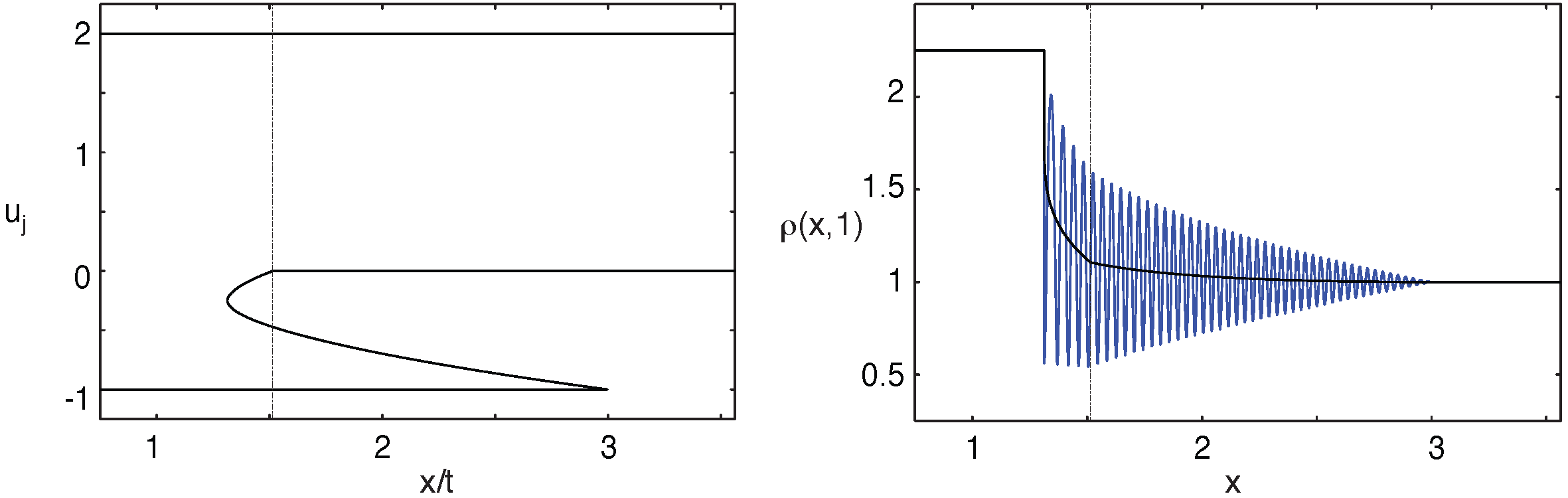
Fig. 7: Self-Similar solution of the Whitham equations (18) with $g=1$ and the corresponding periodic oscillatory solution (21) of the mKdV equation with $\epsilon=0.018$. The initial data is given by (19) with $a=2$, $b=-1$ and $c=0$ of type VI. The oscillations have two distinct structures, which are separated by $x/t\approx 1.51$.

Theorem 13.

(see Figure 7.) For the step-like initial data (19) with $0>a+5b>-4(c-b)$ and $V(a,c,b)<0$, the solution of the Whitham equations (18) with $g=1$ is given by

$$u_{1}=a\ ,\quad\frac{x}{t}=\mu_{2}(a,u_{2},u_{3},b)\ ,\quad\frac{x}{t}=\mu_{3}(a,u_{2},u_{3},b)\ ,\quad u_{4}=b$$ (76)

for $\mu_{3}(a,-(a+b)/4,-(a+b)/4,b)<x/t\leq\mu_{3}(a,u^{***},u^{***},b)$ and by

$$u_{1}=a,\quad u_{2}=c\ ,\quad\frac{x}{t}=\mu_{3}(a,c,u_{3},b)\ ,\quad u_{4}=b$$ (77)

for $\mu_{3}(a,u^{***},u^{***},b)\leq x/t<\mu_{3}(a,c,b,b)$, where $u^{***}$ is the unique solution $u_{3}$ of $\mu_{2}(a,c,u_{3},b)=\mu_{3}(a,c,u_{3},b)$ in the interval $b<u_{3}<c$. Outside the region $\mu_{3}(a,-(a+b)/4,-(a+b)/4,b)<x/t<\mu_{3}(a,c,b,b)$, the solution of equation (17) is given by

$$\alpha=a\ ,\quad\beta=b\quad\mbox{for}\quad\frac{x}{t}\leq\mu_{3}(a,-(a+b)/4,-(a+b)/4,b)\,,$$

and

$$\alpha=a\ ,\quad\beta=c\quad\mbox{for}\quad\frac{x}{t}\geq\mu_{3}(a,c,b,b)\ .$$

Proof.

We first locate the “leading” edge, i.e., the solution of equation (76) at $u_{2}=u_{3}$. Eliminating $x/t$ from the first two equations of (76) yields

$$\mu_{2}(a,u_{2},u_{3},b)-\mu_{3}(a,u_{2},u_{3},b)=0\ .$$ (78)

Since it degenerates at $u_{2}=u_{3}$, we replace (78) by

$$G(a,u_{2},u_{3},b):={\mu_{2}(a,u_{2},u_{3},b)-\mu_{3}(a,u_{2},u_{3},b)\over(u_{2}-u_{3})\sqrt{(u_{1}-u_{3})(u_{2}-u_{4})}I(a,u_{2},u_{3},b)}=0\ .$$ (79)

In the Appendix, we show that, at the “leading” edge $u_{2}=u_{3}$, we have

$$G(a,u_{3},u_{3},b)=2({\partial q\over\partial u_{2}}+{\partial q\over\partial u_{3}})=0\ ,$$

in view of (86), which along with (40) gives $u_{2}=u_{3}=-(a+b)/4$. Having located the “leading” edge, we solve equation (79) near $u_{2}=u_{3}=-(a+b)/4$. We use formula (87) to obtain

$${\partial G(a,-(a+b)/4,-(a+b)/4,b)\over\partial u_{2}}={\partial G(a,-(a+b)/4,-(a+b)/4,b)\over\partial u_{3}}=2\ .$$

These show that equation (79) gives $u_{2}$ as a decreasing function of $u_{3}$

$$u_{2}=B(u_{3})$$ (80)

in a neighborhood of $u_{2}=u_{3}=-(a+b)/4$.

We now extend the solution (80) of equation (78) as far as possible in the region $b<u_{3}<-(a+b)/4<u_{2}<c$. We use formula (37) to obtain

$${\partial\mu_{2}\over\partial u_{2}} = {1\over 2}{\partial\lambda_{2}\over\partial u_{2}}{\partial q\over\partial u_{2}}+{1\over 2}[\lambda_{2}-2(a+u_{2}+u_{3}+b)]{\partial^{2}q\over\partial u_{2}^{2}}\ ,$$

$${\partial\mu_{3}\over\partial u_{3}} = {1\over 2}{\partial\lambda_{3}\over\partial u_{3}}{\partial q\over\partial u_{3}}+{1\over 2}[\lambda_{3}-2(a+u_{2}+u_{3}+b)]{\partial^{2}q\over\partial u_{3}^{2}}\ .$$

In view of (13) and (27), we have

$${\partial\mu_{2}\over\partial u_{2}} > 0\quad\mbox{if}\ \ {\partial q\over\partial u_{2}}>0\ ,$$

$${\partial\mu_{3}\over\partial u_{3}} < 0\quad\mbox{if}\ \ {\partial q\over\partial u_{3}}<0\ .$$

We claim that

$${\partial q\over\partial u_{2}}>0\ ,\quad{\partial q\over\partial u_{3}}<0$$ (81)

on the solution of (78) in the region $b<u_{3}<-(a+b)/4<u_{2}<c$. To see this, we use formula (37) to rewrite equation (78) as

$${1\over 2}[\lambda_{2}-2(a+u_{2}+u_{3}+b)]{\partial q\over\partial u_{2}}={1\over 2}[\lambda_{3}-2(a+u_{2}+u_{3}+b)]{\partial q\over\partial u_{3}}\ .$$

This, together with

$${\partial q\over\partial u_{2}}-{\partial q\over\partial u_{3}}=2(u_{2}-u_{3}){\partial^{2}q\over\partial u_{2}\partial u_{3}}={1\over 2}(u_{2}-u_{3})>0$$

for $u_{2}>u_{3}$, and inequalities (27), proves (81).

Hence, the solution (80) can be extended as long as $b<u_{3}<-(a+b)/4<u_{2}<c$. There are two possibilities; (1) $u_{2}$ touches $c$ before $u_{3}$ reaches $b$ and (2) $u_{3}$ touches $b$ before or simultaneously as $u_{2}$ reaches $c$.

Possibility (2) is unattainable. To see this, we use (53) to write

$$\mu_{2}(a,u_{2},b,b)-\mu_{3}(a,u_{2},b,b)={(u_{2}-b)\over 2(a+u_{2}-2b)}\ V(a,u_{2},b)\ ,$$ (82)

which is negative for $b<u_{2}\leq c$ since $V(a,u_{2},b)$ of (54) is an increasing function of $u_{2}$ and since $V(a,c,b)<0$. Therefore, $u_{2}$ will touch $c$ before $u_{3}$ reaches $b$. When this happens, we have

$$\mu_{2}(a,c,u_{3},b)-\mu_{3}(a,c,u_{3},b)=0\ .$$ (83)

Lemma 14.

Equation (83) has a simple zero, counting multiplicities, in the interval $b<u_{3}<c$. Denoting this zero by $u^{***}$, then $\mu_{2}(a,c,u_{3},b)-\mu_{3}(a,c,u_{3},b)$ is positive for $u_{3}>u^{***}$ and negative for $u_{3}<u^{***}$.

The proof, which involves formulae (51) and (52), is rather similar to the proof of Lemma 73. We will omit it.

We now continue to prove Theorem 4.2. Having solved equation (78) for $u_{2}$ as a decreasing function of $u_{3}$ for $u^{***}<u_{3}<-(a+b)/4$, we can then use the middle two equations of (76) to determine $u_{2}$ and $u_{3}$ as functions of $x/t$ in the interval $\mu_{2}(a,-(a+b)/4,-(a+b)/4,b)<x/t<\mu_{2}(a,c,u^{***},b)$.

We finally turn to equations (77). We want to solve the third equation of (77), $x/t=\mu_{3}(a,c,u_{3},b)$, for $u_{3}<u^{***}$. It is enough to show that $\mu_{3}(a,c,u_{3},b)$ is a decreasing function of $u_{3}$ for $u_{3}<u^{***}$. According to Lemma 4.3, $\mu_{2}(a,c,u_{3},b)-\mu_{3}(a,c,u_{3},b)<0$ for $u_{3}<u^{***}$. Using formula (37) for $\mu_{2}$ and $\mu_{3}$, we have

$${1\over 2}[\lambda_{2}-2(a+c+u_{3}+b)]{\partial q\over\partial u_{2}}<{1\over 2}[\lambda_{3}-2(a+c+u_{3}+b)]{\partial q\over\partial u_{3}}\ .$$

This, together with

$${\partial q\over\partial u_{2}}-{\partial q\over\partial u_{3}}={1\over 2}(c-u_{3})>0$$

for $u_{3}<c$, and inequalities (27), proves

$${\partial q(a,c,u_{3},b)\over\partial u_{3}}<0$$

for $u_{3}<u^{***}$. Hence,

$${\partial\mu_{3}\over\partial u_{3}}={1\over 2}{\partial\lambda_{3}\over\partial u_{3}}{\partial q\over\partial u_{3}}+{1\over 2}[\lambda_{3}-2(a+c+u_{3}+b)]{\partial^{2}q\over\partial u_{3}^{2}}<0\ ,$$

where we have used inequality (13). ∎

4.3 Type VII

Here we consider the step initial function (19) satisfying $0>a+5b>-4(c-b)$ with $V(a,c,b)=0$.

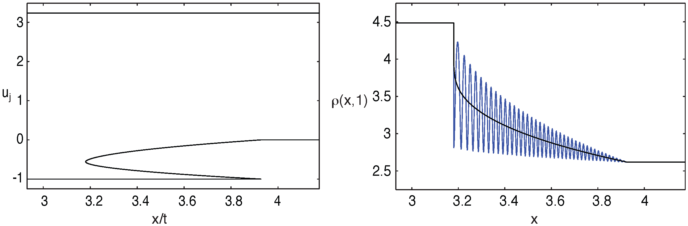
Fig. 8: Self-Similar solution of the Whitham equations (18) $g=1$ and the corresponding oscillatory solution (21) of the mKdV equation with $\epsilon=0.01$. The initial data is given by (19) with $a=1+\sqrt{5}$, $b=-1$ and $c=0$ of type VII.

Theorem 15.

(see Figure 8.) For the step-like initial data (19) with $0>a+5b>-4(c-b)$ and $V(a,c,b)=0$, the solution of the Whitham equations (18) with $g=1$ is given by

$$u_{1}=a\ ,\quad\frac{x}{t}=\mu_{2}(a,u_{2},u_{3},b)\ ,\quad\frac{x}{t}=\mu_{3}(a,u_{2},u_{3},b)\ ,\quad u_{4}=c\,,$$

for $\mu_{3}(a,-(a+b)/4,-(a+b)/4,b)<x/t<\mu_{3}(a,c,b,b)$. Outside the region, the solution of equations (17) is given by

$$\alpha=a\ ,\quad\beta=b\,,\quad\quad\mbox{for}\quad\frac{x}{t}\leq\mu_{3}(a,-(a+b)/4,-(a+b)/4,b)\,,$$

and

$$\alpha=a\ ,\quad\beta=c\,,\quad\quad~{}~{}\mbox{for}\quad\frac{x}{t}\geq\mu_{3}(a,c,b,b)\ .$$

Proof.

It suffices to show that $u_{2}$ and $u_{3}$ of $\mu_{2}(a,u_{2},u_{3},b)-\mu_{3}(a,u_{2},u_{3},b)=0$ reaches $c$ and $b$, respectively, simultaneously. To see this, we deduce from equation (82) that

$$\mu_{2}(a,c,b,b)-\mu_{3}(a,c,b,b)={(c-b)\over 2(a+c-2b)}\ V(a,c,b)$$ (84)

vanishes when $V(a,c,b)=0$. ∎

4.4 Type VIII

Here we consider the step initial function (19) satisfying $0>a+5b>-4(c-b)$ with $V(a,c,b)>0$.

Theorem 16.

(see Figure 9.) For the step-like initial data (19) with $0>a+5b>-4(c-b)$ and $V(a,c,b)>0$, the solution of the Whitham equations (18) with $g=1$ is given by

$$u_{1}=a\ ,\quad\frac{x}{t}=\mu_{2}(a,u_{2},u_{3},b)\ ,\quad\frac{x}{t}=\mu_{3}(a,u_{2},u_{3},b)\ ,\quad u_{4}=b\,,$$

for $\mu_{3}(a,-(a+b)/4,-(a+b)/4,b)<x/t<\mu_{3}(a,\hat{u},\hat{u},b)$, where $\hat{u}$ is the unique $u_{2}$-zero of the quadratic polynomial $V(a,u_{2},b)$ in the interval $-(a+b)/4<u_{2}<c$. Outside the region, the solution of equations (17) is divided into the following three regions:

• For $x/t\leq\mu_{3}(a,-(a+b)/4,-(a+b)/4,b)$,

  $$\alpha=a\ ,\quad\beta=b\,.$$

• For $\mu_{2}(a,\hat{u},b,b)\leq x/t\leq\frac{3}{8}\left(a^{2}+2ac+5c^{2}\right)$,

  $$\alpha=a\,,\quad\beta=-\frac{1}{5}a+\sqrt{\frac{8}{15}\frac{x}{t}-\frac{4}{25}a^{2}}\,.$$

• For $x/t\geq\frac{3}{8}\left(a^{2}+2ac+5c^{2}\right)$,

  $$\alpha=a\,,\quad\beta=c\,.$$

Proof.

By the calculation (84), when $u_{3}$ of $\mu_{2}(a,u_{2},u_{3},b)-\mu_{3}(a,u_{2},u_{3},b)=0$ touches $b$, the corresponding $u_{2}$ reaches $\hat{u}$, where $V(a,\hat{u},b)=0$. Obviously, $\hat{u}<c$. Hence, equations

$$\frac{x}{t}=\mu_{2}(a,u_{2},u_{3},b)\,,\quad\quad\frac{x}{t}=\mu_{3}(a,u_{2},u_{3},b)$$

can be inverted to give $u_{2}$ and $u_{3}$ as functions of $x/t$ in the region $\mu_{2}(a,-(a+b)/4,-(a+b)/4,b)<x/t<\mu_{2}(a,\hat{u},\hat{u},b)$. To the right of this region, equations (17) has a rarefaction wave solution. ∎

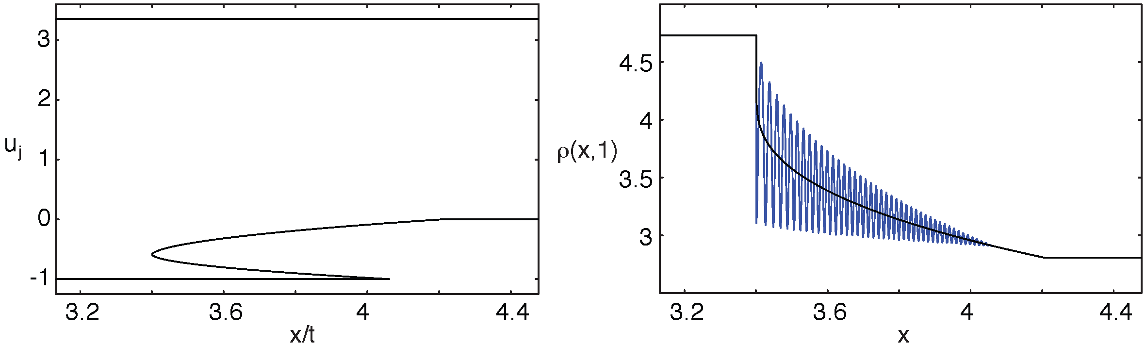
Fig. 9: Self-Similar solution of the Whitham equations and the corresponding oscillatory solution (21) of the mKdV equation with $\epsilon=0.008$. The initial data is given by (19) with $a=4$, $b=-1$ and $c=0$ of type VIII. The solution in the region $4.1<x/t<4.2$ represents a rarefaction wave.

5 Other Initial Data

We conclude the paper by showing how to handle the initial data (20). Inequalities (41) are replaced by

$$\frac{\partial\lambda_{2}}{\partial u_{2}}<\frac{3}{2}\,\frac{\lambda_{1}-\lambda_{2}}{u_{1}-u_{2}}<\frac{\partial\lambda_{1}}{\partial u_{2}}$$

for $u_{4}<u_{3}<u_{2}<u_{1}$. Results similar to Lemma 2.2 can then be easily proved. The rest of calculations are also similar to those in Sections 3 and 4.

Appendix A Leading Edge Calculations

The function $I(u_{1},u_{2},u_{3},u_{4})$ of (24) can be written in terms of the complete elliptic integral of the first kind $K(s)$, i.e.,

$$I={K(s)\over\sqrt{(u_{1}-u_{3})(u_{2}-u_{4})}}\ ,$$

where

$$s={(u_{1}-u_{2})(u_{3}-u_{4})\over(u_{1}-u_{3})(u_{2}-u_{4})}\ .$$

Using the derivative formula

$${dK(s)\over ds}={E(s)-(1-s)K(s)\over 2s(1-s)}\ ,$$

where $E(s)$ is the complete elliptic integral of the second kind, we calculate $\lambda_{2}$ and $\lambda_{3}$ of (23)

$$\lambda_{2} = 2\sigma_{1}-4\ {u_{1}-u_{2}\over 1-{u_{1}-u_{3}\over u_{2}-u_{3}}\ {E\over K}}\ ,$$

$$\lambda_{3} = 2\sigma_{1}+4\ {u_{3}-u_{4}\over 1-{u_{2}-u_{4}\over u_{2}-u_{3}}\ {E\over K}}\ .$$

We then use (37) to write $\mu_{2}-\mu_{3}$ as

$$-2(u_{2}-u_{3})K(s)\left[{u_{1}-u_{2}\over(u_{2}-u_{3})K-(u_{1}-u_{3})E}\ {\partial q\over\partial u_{2}}+{u_{3}-u_{4}\over(u_{2}-u_{3})K-(u_{2}-u_{4})E}\ {\partial q\over\partial u_{3}}\right]\ .$$

Hence, $G(u_{1},u_{2},u_{3},u_{4})$ of (79) becomes

$$G=-2\left[{u_{1}-u_{2}\over(u_{2}-u_{3})K-(u_{1}-u_{3})E}\ {\partial q\over\partial u_{2}}+{u_{3}-u_{4}\over(u_{2}-u_{3})K-(u_{2}-u_{4})E}\ {\partial q\over\partial u_{3}}\right]\ .$$ (85)

We now use the asymptotics of $K(s)$ and $E(s)$ as $s$ is close to $1$

$$K(s)\approx\frac{1}{2}\log\frac{16}{1-s}\ ,\quad E(s)\approx 1+\frac{1}{4}(1-s)\left(\log\frac{16}{1-s}-1\right)$$

to calculate the $u_{2}=u_{3}$ limit

$$G=2\left({\partial q\over\partial u_{2}}+{\partial q\over\partial u_{3}}\right)\ .$$ (86)

Finally, we can also use the expression (40) and the derivative formula

$${dE(s)\over ds}={E(s)-K(s)\over 2s}$$

to evaluate the partial derivatives of $G$ in the $u_{2}=u_{3}$ limit

$${\partial G\over\partial u_{2}}\Big{|}_{u_{2}=u_{3}} =2+{(u_{1}-u_{4})(u_{1}+4u_{3}+u_{4})\over 4(u_{1}-u_{3})(u_{4}-u_{3})}\ ,$$ (87)

$${\partial G\over\partial u_{3}}\Big{|}_{u_{2}=u_{3}} =2-{(u_{1}-u_{4})(u_{1}+4u_{3}+u_{4})\over 4(u_{1}-u_{3})(u_{4}-u_{3})}\ .$$

Acknowledgments. We thank Ed. Overman for showing us his numerical simulations of the NLS and mKdV equations for small dispersion. Y.K. and F.-R. T. were supported in part by NSF Grant DMS-0404931 and V.P. was supported in part by NSF Grant DMS-0135308.

References

• [1] P. Deift, S. Venakides and X. Zhou, New results in small dispersion KdV by an extension of the steepest decent method for Riemann-Hilbert problems, International Math. Research Jour., 4(1997), pp. 285-299.
• [2] B.A. Dubrovin and S.P. Novikov, Hydrodynamics of weakly deformed soliton lattices. Differential geometry and Hamiltonian theory, Russian Math. Surveys 44:6(1989), pp. 35-124.
• [3] G. A. El, V. V. Geogjaev, A. V. Gurevich and A. L. Krylov, Decay of an initial discontinuity in the defocusing NLS hydrodynamics, Physica D, 87(1995), pp. 186-192.
• [4] M.G. Forest and J. Lee, Geometry and modulation theory for periodic nonlinear Schrödinger equation, in Oscillation Theory, Computation and Method of Compensated Compactness, J.L. Ericksen, D. Kinderlehrer, and M. Slemrod eds., Springer-Verlag, 1986, pp. 35-69.
• [5] T. Grava and C. Klein, Numerical solution of the small dispersion limit of Korteweg-de Vries and Whitham equations, Comm. Pure Appl. Math., 60(2007), pp. 1623-1664.
• [6] S. Jin, C.D. Levermore and D.W. McLaughlin, The semiclassical limit of the defocusing NLS hierarchy, Comm. Pure Appl. Math., 52(1999), pp. 613-654.
• [7] Y. Kodama, The Whitham equations in optical communications: mathematical theory of NRZ, SIAM J. Appl. Math., 59(1999), pp. 2162-2192.
• [8] P.D. Lax, C.D. Levermore and S. Venakides, The generation and propagation of oscillations in dispersive IVPs and their limiting behavior, in Important Developments in Soliton Theory 1980-1990, T. Fokas and V.E. Zakharov eds., Springer Series in Nonlinear Dynamics, Springer, Berlin, 1993, pp. 205-241.
• [9] V. B. Matveev, Abelian functions and solitons, preprint no. 373, University of Wroclaw, Wroclaw, 1976.
• [10] M.V. Pavlov, Nonlinear Schrödinger equation and the Bogolyubov-Whitham method of averaging, Theor. Math. Phys., 71(1987), pp. 584-588.
• [11] V. U. Pierce and F.R. Tian, Self-Similar solutions of the non-strictly hyperbolic Whitham equations, Comm. Math. Sci., 4(2006), pp. 799-822.
• [12] V. U. Pierce and F.R. Tian, Self-similar solutions of the non-strictly hyperbolic Whitham equations for the KdV hierarchy, Dynamics of PDE, 4(2007), pp. 263-282.
• [13] F.R. Tian and J. Ye, On the Whitham equations for the semiclassical limit of the defocusing nonlinear Schrödinger equation, Comm. Pure Appl. Math., 52(1999), pp. 655-692.
• [14] F.R. Tian, The Whitham type equations and linear overdetermined systems of Euler-Poisson-Darboux type, Duke Math. Jour., 74(1994), pp. 203-221.
• [15] S.P. Tsarev, Poisson brackets and one-dimensional Hamiltonian systems of hydrodynamic type, Soviet Math. Dokl., 31(1985), pp. 488-491.
• [16] S. Venakides, Higher order Lax-Levermore theory, Comm. Pure Appl. Math., 43(1990), pp. 335-362.